Investigation of Shock Wave Oscillation Suppression by Overflow in the Supersonic Inlet

Abstract

With a focus on the shock oscillation phenomenon of a supersonic inlet at a high Mach number, the influence of isolator overflow on shock oscillation is studied in this paper. The shock wave dynamic model with overflow was established by the theoretical method, and the integrated numerical model of internal flow and external flow in the inlet was established too. The theoretical analysis of rate of overflow and overflow position on the flow field is carried out, and the changes of flow field parameters are studied by numerical simulation under different overflow positions. The results showed that both increasing the rate of overflow and setting the overflow gap close to the shock front were beneficial to reducing the flow parameters’ oscillation. In the viscous flow field, the overflow gap restricted the forward development of the local separation region of the shock train system, thus constraining the shock wave movement process, which could significantly reduce the parameter oscillation. In model C with two groups of overflow gaps, pressure oscillations of sampling point P_U8 and P_L8 were reduced to 29.81% and 30.56% relative to without overflow, and the corresponding rate of overflow was within 3.6%, which indicated that the appropriate overflow gap setting could effectively suppress the self-excited oscillation in the inlet.

1. Introduction

The shock/boundary layer interaction is an important flow phenomenon in supersonic and hypersonic inlets [1], which also generally exists in supersonic pipeline flows [2], such as the nozzle flow [3]. When the combustor backpressure becomes higher, the backpressure shock moves forward, and the shock evolves into a complex shock train system [4,5,6], so an equal cross-sectional area isolator is usually set to hold the shock train [7,8]. With increasing flight speed, the shock train easily shows an unsteady oscillation feature [9,10,11], which will damage the inlet structure and reduce the engine performance. Therefore, the study of shock wave oscillation suppression in the supersonic and hypersonic inlet has drawn extensive attention.

The cause and transmission mechanism of shock wave oscillation in the supersonic inlet have been investigated by many researchers [12,13,14]. Characteristic parameters of shock wave oscillation, such as frequency, were obtained with theoretical analysis [15,16]. Much research has also been carried out on the dynamic characteristics of shock waves by numerical simulation and experiment. Wagner [17] studied the inlet unstart state and found that the unstart process is closely related to the boundary layer separation and the motion characteristics of the shock train, and that three unstart states have different dynamic characteristics. Tan [18] observed the low-frequency large oscillation of the shock train in the hypersonic inlet through experiments and analyzed the relationship between the main oscillation frequency and the boundary layer. Tian et al. [19] studied the flow structure and dynamic characteristics of the oblique shock train under two different backpressure states. The results showed that the forward movement process of the shock train has two states: stable forward movement and sharp forward movement. Li et al. [14] used theoretical modeling of the motion of the shock train leading edge in complex background waves, which better predicted the characteristics of the rapid forward propagation of the shock train. Lu Lei [20] studied the RBCC inlet and found that with the back pressure increasing, the forward transmission process of the shock train includes four motion periods. Each motion period contains two motion modes: slow forward transmission and “sudden jump” forward transmission. The shock train structure presents the characteristics of “spring”. These studies have continuously deepened the understanding of shock wave motion.

The unsteady oscillation processes of the shock train usually occur in supersonic and hypersonic inlets, which have adverse effects on engine performance. Additionally, the active suppression measure is usually required. Flow control is often carried out for boundary layer flow, including the passive flow control method [21] and the active flow control method, such as the jet control [22], the suction control [23] and so on. As an extensively used active flow control technology, the boundary layer suction has a broad prospect in suppressing the boundary layer separation [24,25] and could improve the backpressure inhibition ability of the inlet [26]. Ma et al. [27] studied the suppression effect of boundary layer suction on shock wave oscillation in the compressor, which showed that the suction influences oscillation frequency and relative amplitude with an apparent effective threshold value, and the suction will produce a good effect within the threshold value while reducing the compressor performance exceeding the threshold value. Cravero et al. [28] investigated a centrifugal compressor scheme with an orifice shroud and showed that under near-surge conditions, by circulating a low momentum flow in the passive cavity, the main flow was reactivated, which significantly increased pressure ratio. Herrmann [29] conducted an experimental study on the supersonic inlet with suction and found that the shock train oscillated downstream the suction gap when the backpressure was lower, while the shock train moves forward to the suction gap and is constrained to oscillate near the suction gap when the backpressure was higher. Huang et al. [30] experimentally studied an inlet with a suction gap, which showed that the unsteady shock train oscillation with the influence of the suction gap was very complex, and different blockages led to two modes: large-amplitude oscillation and small-amplitude oscillation. In these research works above, for the boundary layer suction of the supersonic inlet, the main goal is to control the local separation flow in the supersonic compression section of the inlet. The overflow devices are concentrated in the front of the isolator of the supersonic inlet to suppress the shock wave oscillation under high back pressure. However, under self-excited oscillation, when the shock train is located in the middle and downstream of the isolator section, the overflow at the front of the isolate has little influence on the shock train. The suppression method by overflow in the middle and downstream of the isolator, and the influence of overflow position, rate of overflow and other parameters on oscillation have not been fully studied.

The shock wave oscillation influenced by a boundary layer overflow in the supersonic inlet is studied in this paper. Unlike previous studies, some overflow devices are set along the shock train region. The influence of overflow on shock wave oscillation is analyzed with the shock wave dynamics model. The processes of viscous flow field structure evolution and parameter oscillation are investigated with numerical simulation. The suppression on the shock oscillation process by overflow in the isolator section is studied, and the effects of the overflow position and rate of overflow on the flow parameters are analyzed, which provides a new technical approach to suppress the self-excited oscillation of the supersonic inlet.

2. Methodology

2.1. Geometric Model

The research is carried out with the inlet in reference [31] as the object, which is often used to verify numerical simulation methods [32], and the inlet profile is shown in Figure 1. The height of the inlet H₁ = 29 mm, the first-stage compression angle δ₁ = 20.5°, the length of the equal-straight isolator L₂ = 79.4 mm, the height of the isolator H₂ = 15 mm, and the angle of the expansion section δ₃ = 5°. Other geometric parameters are consistent with those in reference [31]. Overflow devices are all set in the isolator.

Based on the basic model, the inhibitory effect of the isolator overflow on shock oscillation is studied. An overflow gap is set on the lower wall of the isolator. The overflow gap is perpendicular to the flow direction and is located in the middle and the end of the isolator, respectively. The width L₄ and spacing L₅ of each gap are 0.75 mm, and the spacing of two overflow gaps L₆ = 24.75 mm.

In the numerical simulation process, 16 equally spaced sampling points are set in the inner channel of the inlet, which are distributed on the upper and lower walls to monitor the change of pressure, as shown in the Figure 2. The two gap groups are Gap_1 and Gap_2, respectively. The total length of the sampling area is 52.5 mm, and the sampling point spacing is 7.5 mm, which are P_U1~P_U8 and P_L1~P_L8 from front to back. The P_L5 and P_L8 points are behind the two overflow positions, respectively.

2.2. Iso-Straight Channel Shock Dynamics Model

Firstly, the theoretical method is used to establish the normal shock wave dynamics model in the channel with constant cross section, so as to study and analyze the influence law of the overflow on the shock wave motion and parameter changes.

In the model in Figure 3, shock wave 1 is used as the interface, and the pipe flow is divided into two regions: upstream U and downstream D. The velocities of the pipe entrance and export are Ma₁ and Ma₂, respectively; the external environment V is connected to the channel through the gap, In the modeling process, the rear control body is composed of shock surface 1, export face 2 and the pipe wall. The modeling is divided into two cases according to whether there is overflow.

2.2.1. No Overflow Model

The propagation velocity of the steady-state shock wave in the channel subjected to upstream or downstream disturbance is [33]:

$$v_s=a_{1U}\sqrt{\frac{p_{1D}}{p_{1U}}\frac{k+1}{2k}+\frac{k-1}{2k}}$$

(1)

where P_1U and P_1D are the upstream and downstream pressures, a_1U is the upstream sound velocity. Ma_1U is the upstream Mach number, k is the adiabatic index. According to the shock wave propagation speed, the moving speed of the shock surface is calculated as:

$$\dot{x}=a_{1U}\left(M{a}_{1U}-\sqrt{\frac{P_{1D}}{P_{1U}}\frac{k+1}{2k}+\frac{k-1}{2k}}\right)$$

(2)

Define parameters Ma_M: $M{a}_M=M{a}_{1U}-{\dot{x}}_1/a_{1U}$

Calculate the downstream flow ${\dot{m}}_{1D}$ of shock wave according to the aerodynamic parameters and at the upstream:

$${\dot{m}}_{1D}={\dot{m}}_{1U}\left(1+\frac{1}{a_{1U}M{a}_{1U}}\frac{2\left(M{a}_M^2-1\right)}{2+\left(k-1\right)M{a}_M^2}{\dot{x}}_1\right)$$

(3)

The relationship between the volume change rate in the downstream region D of the shock wave and the shock wave speed is:

$${\dot{V}}_D=-A{\dot{x}}_1$$

(4)

According to the ideal gas equation:

$${\rho }_D=\frac{M{P}_D}{R{T}_D}$$

(5)

Here, R is the gas constant of the ideal gas.

The flow rates of the entrance and export flowdownstream of the shock wave are as follows:

$${\dot{m}}_{1D}-{\dot{m}}_2=V_D{\dot{\rho }}_D+{\rho }_D{\dot{V}}_D=V_D\frac{M}{R{T}_D}{\dot{P}}_D+\frac{M{P}_D}{R{T}_D}{\dot{V}}_D$$

(6)

From Equations (2)–(6), including eight parameters such as ${\dot{x}}_1$, $P_D$, ${\dot{P}}_D$, $V_D$, ${\dot{V}}_D$,${\rho }_D$, ${\dot{\rho }}_D$ and $T_D$, the integral equation is supplemented:

$$\left\{\begin{array}{l}{P}_D={\displaystyle \int {\dot{P}}_D}dt\\ V_D={\displaystyle \int {\dot{V}}_D}dt\\ {\rho }_D={\displaystyle \int {\dot{\rho }}_D}dt\end{array}\right.$$

(7)

The parameter calculation model of the upstream control body is similar to that of the downstream. For the above differential equations, the change process of shock motion parameters can be solved by simultaneous solutions.

2.2.2. Overflow Model

When the overflow device is located in front of the shock surface 1 (Figure 3), that is, the region U, it does not affect the downstream D parameters; when the overflow device is behind the shock surface, the flow overflowing from the control body D to the outward flow field V is:

$${\dot{m}}_V=K\frac{P_D}{\sqrt{T_D}}q\left({\lambda }_{Gap}\right)A_{Gap}$$

(8)

Among them, A_Gap is the gap area, and λ_Gap is the velocity coefficient of the gap flow, which corresponds to the flow velocity Ma_Gap.

According to the relationship between the pressure inside and outside the channel, the flow Mach number Ma_Gap is calculated in two cases:

I: $P_D>P_V$ and $P_D<1.8929P_V$

In this case, the flow in the gap does not reach the sound velocity, and the flow velocity is calculated according to the following equation:

$$M{a}_{Gap}=\sqrt{\left({\left(\frac{P_V}{P_D}\right)}^{-\frac{k-1}{k}}-1\right)/0.2}$$

(9)

II: $P_D\ge 1.8929P_V$

$$M{a}_{Gap}=1.0$$

(10)

When there is overflow, Equation (6) is changed to:

$${\dot{m}}_{1D}-{\dot{m}}_V-{\dot{m}}_2=V_D\frac{M}{R{T}_D}{\dot{P}}_D+\frac{M{P}_D}{R{T}_D}{\dot{V}}_D$$

(11)

By combining Equations (8)–(11) with the no-overflow model, the downstream region D parameter changes of the shock wave under overflow conditions can be solved.

2.2.3. Steady-State Parameter Verification

According to the established shock wave dynamics equation, the calculation program is written in C++ language. The steady-state parameters are calculated and compared with the shock wave theoretical results. The calculated parameters are: entrance speed Ma₀ = 2.5, sound speed a₀ = 299.46 m/s, total temperature 502.088 K and entrance flow 3.092 kg/s.

In the calculation process, according to the given entrance parameter value, three working conditions of the deviation of the entrance and export pressure from the theoretical value are set, and the steady-state value is calculated according to the shock wave dynamics model in Section 3.1. By comparing the three working conditions, it can be seen from

Table 1. Calculation of parameters after shock wave.

	Theoretical Value	Dynamic Shock Model Values
△P0 (%)	---	−10	10	15
△P2 (%)	---	10	−10	0
P0 (Pa)	26,465	26,465	26,465	26,465
P2 (Pa)	188,357	188,564	188,564	188,564
Ma2	0.513	0.513	0.513	0.513
P2* (Pa)	225,943	225,645	225,645	225,645

that under different initial value errors, the parameters such as pressure P₀ and P₂, velocity Ma₂ and total pressure P₂^* after normal shock wave all converge to the same steady-state value, which is consistent with the calculation results of shock wave theory.

2.3. Numerical Modeling

2.3.1. Numerical Method and Mesh

Because the viscous flow field in the inlet is very complex, the theoretical model cannot reflect the flow details. The numerical simulation method is used to analyze the characteristics of the flow field, and the influence of the overflow on the parameters of the viscous flow field is studied.

Firstly, according to the basic model shown in Figure 1, a numerical model of flow field numerical simulation (CFD: computational fluid dynamics) is established. The internal and external flow integrated model of the inlet flow field and the external flow field is established, and the finite volume method is used to solve the control equation. For the internal flow field including shock wave, expansion wave, shock wave/boundary layer interaction, high reverse pressure gradient and other complex flow phenomena, the SST k-ω model can better simulate the separated flow with a strong reverse pressure gradient, which is widely used in calculations [34]. Therefore, the SST k-ω model is adopted in this paper. The commercial software ANSYS Fluent was used to solve the Reynolds Averaged Navier–Stokes equations.

The inlet flow field is divided into structured meshes as shown in Figure 4; the inner flow field is fine, while the outer flow field is sparse. At the same time, mesh refinement in the area near the wall and overflow gap of inner channel. In order to compare the influence of different mesh accuracy on the flow field calculation, three models with different numbers of meshes are established. The number of meshes for the base model is 300,000 (CFDMeshA). Based on the basic model, the regions such as boundary layer and overflow gap are refined, and two models with 340,000 meshes (CFDMeshB) and 360,000 meshes (CFDMeshC) are generated; the improved model guarantees that y+ is between 1 and 2. The boundary conditions of the calculation area mainly include three types: the side and entrance A of the external flow field is the pressure far-field boundary; The export B of external flow field and export B of supersonic inlet are the pressure outlet boundary, and the wall C of supersonic inlet is the wall boundary, as shown in Figure 4.

2.3.2. Numerical Model Verification

According to the test conditions in reference [31], the verification and analysis are carried out for the working conditions of the incoming flow Ma₀ = 2.41.

From the wall pressure distribution in Figure 5, the wall pressure fluctuates due to the complex shock wave system in the flow field. The pressure at most points is in good agreement with the test results, which better reflects the pressure change process. By comparing the calculation results of the three models, we can see that the change trends are consistent, except that the curve of the pressure jump point generated by the shock wave is slightly different, and other areas show basically the same trend. The local differences between MeshB and MeshC are small, which indicates that wall boundary layer mesh densification is necessary for the simulation of shock/boundary layer interaction.

Figure 6a compares the Mach number contour of numerical simulation and experimental schlieren when Ma₀ = 2.41. It can be seen that the shock wave systems of the two results are basically the same, and the local expansion at the turning point of the upper compression surface, shock wave/boundary layer interaction, shock wave/expansion wave system and reflection are well reflected by numerical simulation. This shows that the numerical modeling method in this paper is feasible.

In reference [31], experiments and simulation calculations were carried out for the state of Ma₀ = 3.00, and the comparison showed that the shock wave system calculated by numerical simulation was close to the experimental results. Figure 6b compares the numerical simulation results of this paper with the reference. It can be seen that the shock wave reflected by the lower lip after the increase of the incoming flow velocity induces a larger separation area at the turning point of the upper wall surface, as well as the local expansion waves and shock waves generated by the influence of the separation zone on the incoming flow. In addition, shock wave reflections are generated in the iso-straight section and the expansion section. These flow phenomena and shock wave systems are consistent with the results in reference [31].

2.3.3. Computational Model and Time Step

When Ma₀ = 3.00, the total pressure is 620 kPa, the total temperature is 290 K and the backpressure is 9.0 times the incoming flow pressure. According to the research, the oblique shock wave system exhibits self-excited oscillation under fixed backpressure.

The shock wave dynamics theoretical calculation shows that both the overflow location and the gap ratio have an effect on the shock wave oscillation. Based on the basic model of the inlet, an overflow channel is set, one is located at the export of the equal straight section of the inlet (Gap_1), and the other is set in the leading-edge area of the shock system, that is, the middle of the isolator (Gap_2).

Table 2. Calculation Model.

Model	Overflow Devices
A	/
B	Gap_1
C	Gap_1, Gap_2

gives the calculation models of the three combinations of overflow devices.

The time step size is very important for the unsteady flow field simulation. According to Wong’s [35] relationship between the oscillation frequency of the pipeline shock train and the flow field parameters:

$$f_r=\frac{a\left(1-M{a}_2^2\right)}{4L}$$

(12)

Here, a and Ma₂ are the sound speed and Mach number behind the shock wave, respectively, and L is the axial distance between the first oblique shock wave and the pipe export.

According to the equation above, parameters behind the shock wave need to be calculated. Since the distribution of parameters behind the shock wave is uneven and periodically oscillates along with the time, the theoretical relationship cannot reflect the parameter distribution. Therefore, parameters behind the shock wave are calculated by the shock wave theory with the average value of the steady flow field before the shock wave. So, the average velocity before the shock Ma₁ = 2.002, the static temperature T = 173.27 k, the sound velocity after the shock a = 343.01 m/s, the average velocity Ma₂ = 0.577, and the average distance between the shock position and the flow channel export L = 0.12 m. As a result, the first-order oscillation frequency of the flow field is 476.7 HZ.

At this frequency, it is guaranteed that there are no less than 4000 time steps in one oscillation period, and the time step size for unsteady calculation is determined to be 0.5 × 10⁻⁶ s. The steady model is first used for calculation, then the unsteady calculation is transferred after the flow field is established.

3. Results and Discussion

3.1. Theoretical Analysis of Influence of Overflow Parameters on Shock Oscillation

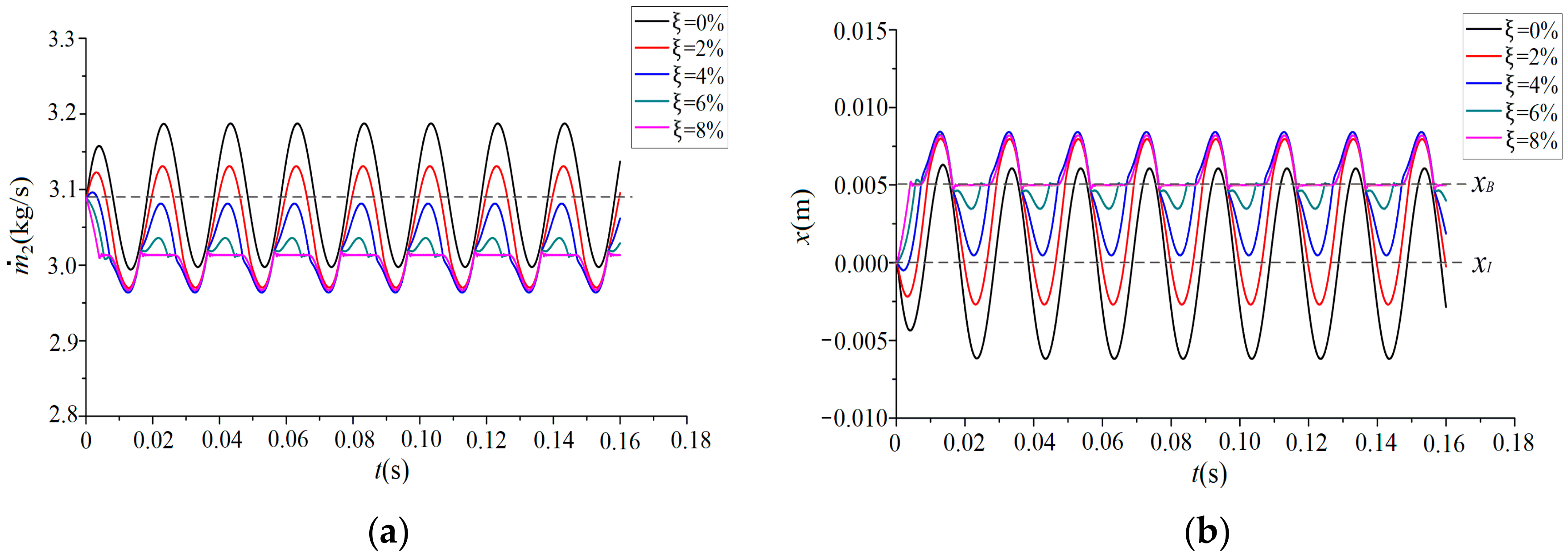
3.1.1. Influence of Overflow Gap Ratio

For different overflow gap to throat area ratios ξ = A_Gap/A₂ and the periodic change of backpressure P₂, the changes of export flow ${\dot{m}}_2$ and shock position x₁ with the time are analyzed. The overflow gap is 0.005 m downstream of the forward wave surface, and the variation law of backpressure is as follows:

$$P_2=P_{2S}+0.05P_{2S}sin\left(100\pi t\right)$$

(13)

Here, P_2s is the steady-state export pressure calculated according to Section 2.2.3.

Firstly, the flow process with the overflow gap is analyzed. The shock wave movement process is shown in Figure 7. Among them, A-D represents the change relationship between the shock wave position and motion direction with the outlet pressure P₂ in a cycle. When the export pressure decreases, the normal shock wave moves backward and crosses the overflow gap under low backpressure, as shown in Figure 7A. Due to the small pressure difference between the pressure before the shock wave and the ambient pressure, the export velocity Ma_Gap of the gap decreases. In the period of pressure rise (Figure 7B), when the backpressure rises, the normal shock wave is pushed to the entrance direction. When the shock wave surface crosses the overflow gap, due to the significant increase of pressure after the normal shock wave, the pressure difference inside and outside the overflow gap increases sharply, the gap Ma_Gap increases, and even reaches the choked flow state. At this time, the forward movement of the shock wave is “blocked” due to partial flow overflow. Further increasing the export pressure, the shock wave continued to move forward (Figure 7C). When the export pressure drops to a certain value, the shock wave moves back to the overflow gap, and the pressure on both sides of the overflow gap also decreases, and the flow velocity decreases (Figure 7D).

From the flow change law in Figure 8a, due to the periodic change of export pressure, the flow also shows a periodic change law. The first cycle is the parameter establishment process, and its amplitude change is different from the subsequent fluctuation. When ξ = 0, the export flow ${\dot{m}}_2$ changes periodically with the export pressure change and the flow curve changes periodically above and below the steady-state value.

Compare the shock position curve in Figure 8b, where x_I and x_B are the initial shock wave position and the overflow position, respectively. When ξ > 0, the periodic motion of the flow changes. When ξ = 2% and ξ = 4%, export flow and shock position changes are still approximately sine curves, but the amplitude decreases with ξ increasing. At the same time, since the overflow gap is located downstream of the shock wave, after overflowing through the gap, the mean value of the export flow ${\dot{m}}_2$ decreases, and the average position of the shock wave oscillation also moves backward. When ξ = 6%, the amplitude of the flow curve is tiny, and the law of sinusoidal oscillation is changed, and the shock wave oscillates slightly around the overflow position. As ξ increases further to 8%, the shock wave moves forward to the overflow position, but the gap prevents shock wave from continuing to move forward. So, the shock wave keeps a “locked” state, and the corresponding export flow remains unchanged. When the backpressure drops, the shock wave moves backward again, so that the flow and shock position have only half amplitude oscillation.

The oscillation amplitudes of the flow and the shock position changing with ξ are compared in

Table 3. Parameters amplitude variation under different ξ.

ξ (%)	0	2	4	6	8
$\Delta {\dot{m}}_2$ (kg/s)	0.1898	0.1606	0.1176	0.0691	0.0506
$\Delta x_{shock}$ (m)	0.01226	0.01066	0.00795	0.00473	0.00344

. The overflow significantly affects the shock wave position oscillation and the export flow oscillation. When ξ = 8%, the oscillation amplitude of the export flow is only 27% of the no-overflow state, and the oscillation amplitude of the shock wave position also drops to 28%.

3.1.2. Influence of Overflow Position

As shown in Figure 7, the influence of the overflow position on the flow field parameters is different when the overflow position is upstream or downstream the shock wave. Taking ξ = 6% as an example, the relationship between the initial position x_I and overflow position x_B of five different shock waves is analyzed as follows:

It can be seen from the curve in Figure 9 that the relative position Δx influences the flow fluctuation, and the mean value of the export flow ${\dot{m}}_2$ and the shape of the curve both change with the time. When Δx = −0.005 m, the overflow gap is before the initial position of the shock wave. Along with the backpressure rising, the shock wave moves forward to the overflow gap, then its position remains unchanged, the curve is locally flat, and the corresponding local flow rate also remains unchanged. When x = 0 m, the position and the flow of the shock wave show sinusoidal oscillation during the shock wave backward movement, while the shock wave is “locked” at the gap position when the shock wave moves forward, and the export flow ${\dot{m}}_2$ and the shock wave position x remain unchanged. When Δx increases further to 0.015 m, the flow and position curves oscillate sinusoidally, while the shock wave “locks” when it moves backward to the overflow position, and the upper half of the flow and position curves remain flat. In addition, as Δx increases, the overall position of the shock wave moves backward, and the average flow decreases. Nevertheless, from the perspective of amplitude, when Δx = 0.005 m, the fluctuation of flow and shock wave position is the smallest. It can be seen from the results that the gap can hinder and suppress the shock oscillation, which is related to the value of Δx.

3.2. Calculation and Analysis of Viscous Flow Field

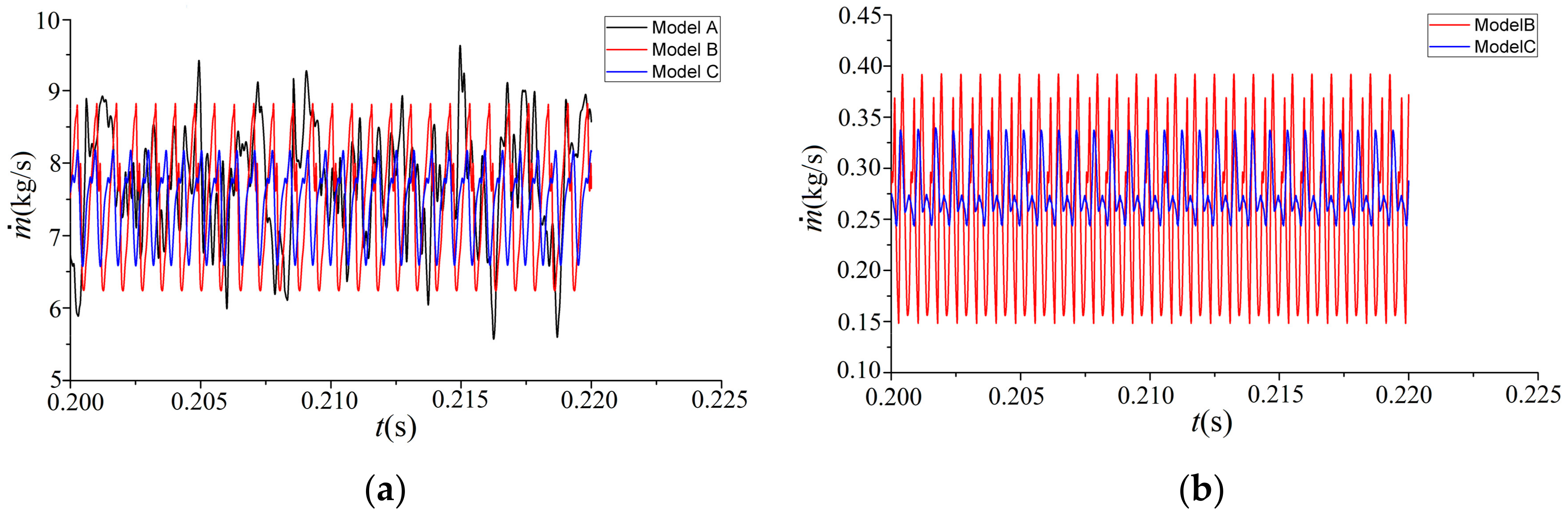
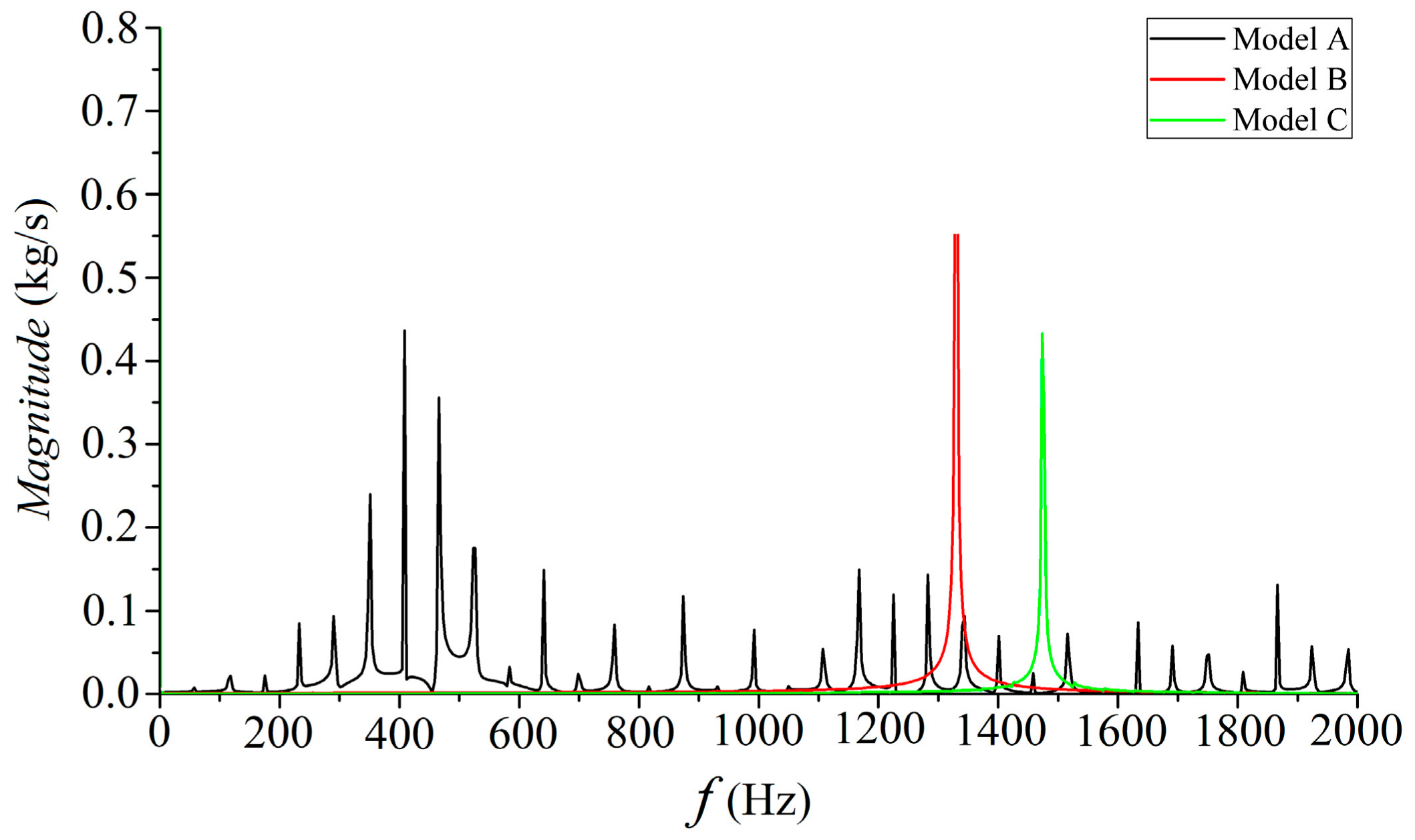
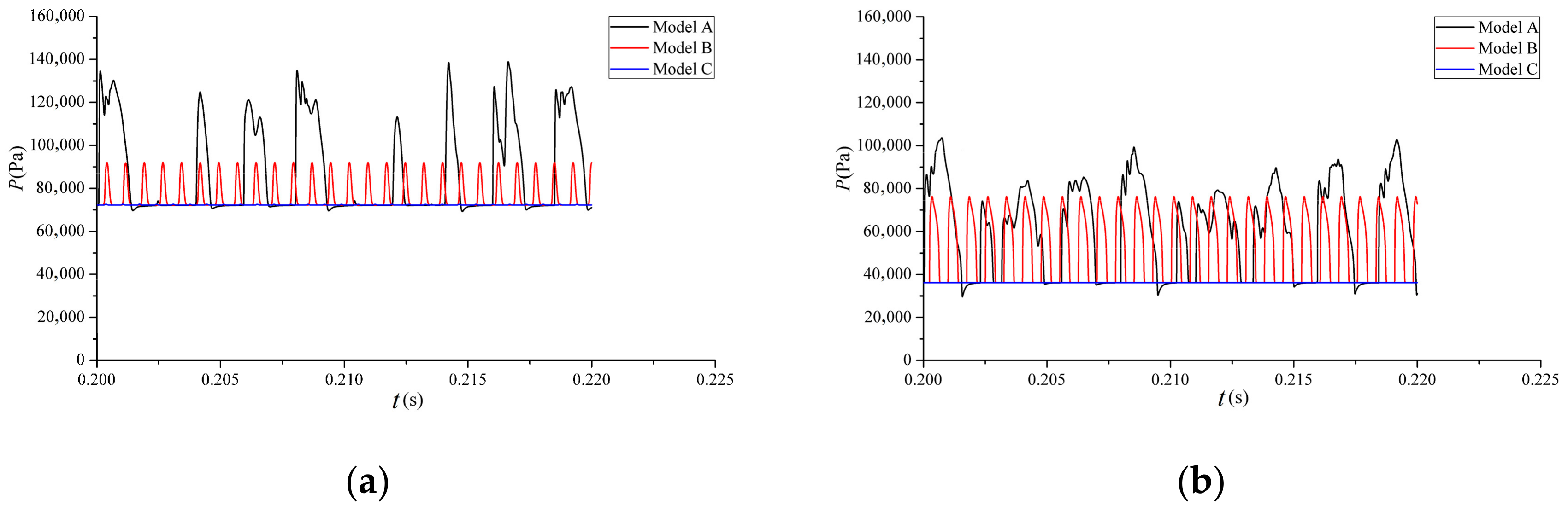
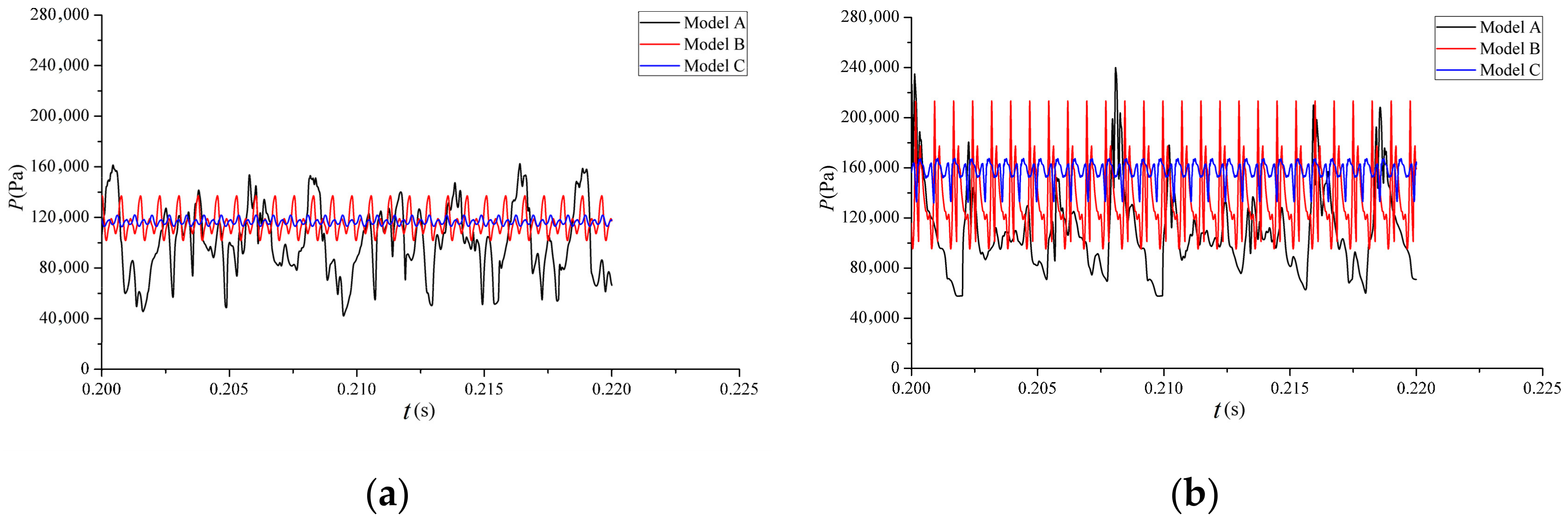
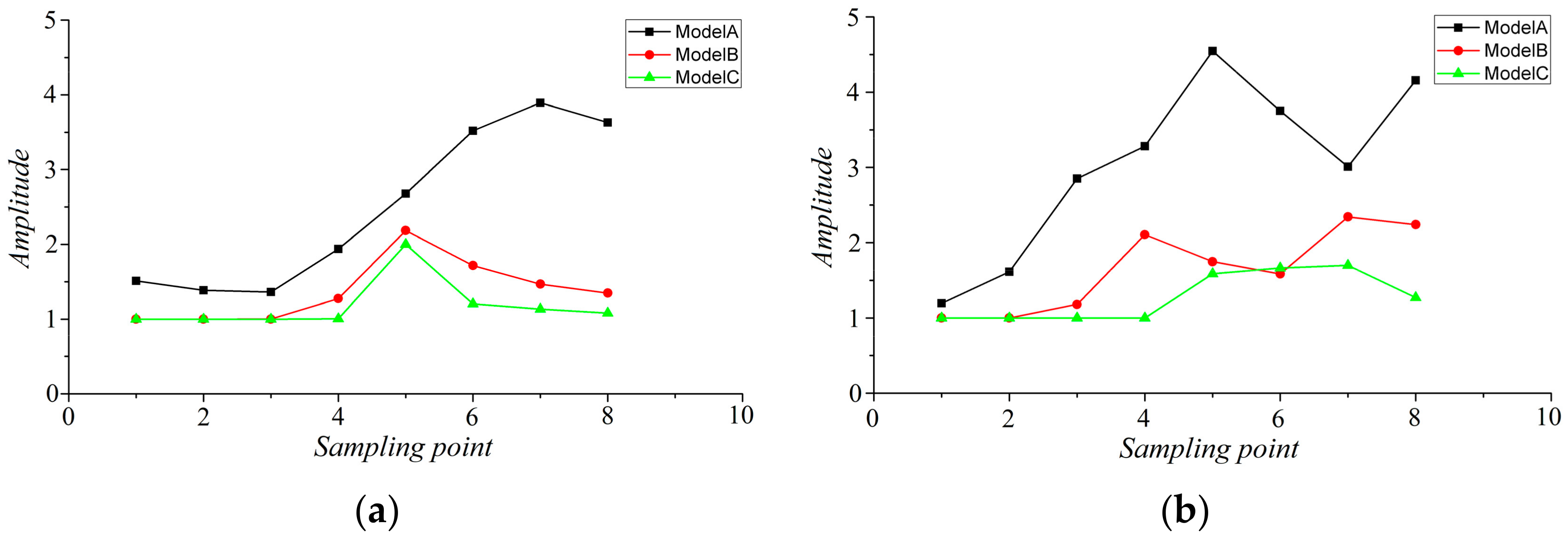
3.2.1. Calculation and Analysis of Flow Field Parameter Oscillation

Unsteady calculation is carried out for the three models in Table 2. Figure 10a compares the change process of the export flow of the inlet under the three working conditions. It can be seen that the export flow curve oscillates due to the shock wave self-excited oscillation in the flow field. In Model A without overflow, the export flow fluctuates and has obvious aperiodicity. The flow fluctuates greatly over time, and the maximum fluctuation is more than 4.05 kg/s. The impact of overflow on the export flow is very significant. On the one hand, the export flow has periodic fluctuations with good consistency, and the oscillation amplitude of the flow curve decreases from modal A to modal C. The maximum flow ranges of Model B and Model C are 2.59 kg/s and 1.61 kg/s, respectively. On the other hand, the oscillation frequency of the export parameters increases significantly, which is quite different from Model A.

The mass from the overflow gap exhibits periodic changes (Figure 10b). Model C is equipped with two overflow devices, which is much more effective on oscillation suppression. Corresponding to the export flow, the flow oscillation range of the overflow channel is small, and the oscillation amplitudes of the two working conditions are 0.2443 kg/s and 0.0962 kg/s, respectively. Due to the increase in the number of overflow gaps in Model C relative to Model B, the average rate of overflow increased from 0.2574 kg/s to 0.2781 kg/s, a relative increase of about 8%. Through the analysis of the results of Model C, the flows of the front and back overflow gaps are different. Due to the compression and pressurization effect of the shock train, the back overflow gap Gap_1 is always in the region where the shock train enhances the compression. Affected by the large pressure difference between the internal and external flow fields, the rate of overflow is larger. The average flows of the front and back overflows are 0.05879 kg/s and 0.2193 kg/s, respectively, and the back suction gaps account for 78.86% of the total suction flow. From the calculation results, the average rate of overflow in the time sense of Model B and Model C accounts for 3.32% and 3.59% of the mainstream, and the overflow is not large.

For the above three working conditions, the spectrum analysis of the flow is carried out, as shown in Figure 11. In the Model A model, the first-order frequency is about 415 Hz, which is slightly different from Equation (12) and the simulation calculation results in reference [35]. In addition to the first-order frequencies, the spectrum also shows several frequency points with high amplitude in 300 Hz~600 Hz. This means that the shock oscillation has non-periodic characteristics, which is similar to the shock motion divided into long-period and short-period motion and shock jumps proposed in references [14,36]. When there is a suction gap, the periodic fluctuation of the flow is evident. In the spectrum analysis, the first-order main frequency of Model B and Model C is the most important component, while the amplitudes at other frequencies are very low. After FFT analysis, the flow oscillation frequencies of Model B and Model C are 1328 Hz and 1473 Hz, respectively. Compared with the working condition without suction, the oscillation frequency of the export flow increased significantly. In terms of amplitude, the main frequency amplitude of Model B is higher than that of Model A: furthermore, Model C is similar to Model A. However, many frequency points in Model A have larger amplitudes. The mean flows of the three models are 7.7476 kg/s, 7.4865 kg/s and 7.4647 kg/s, respectively.

Figure 12 and Figure 13 show the pressure comparison of sampling point 4 and sampling point 8, respectively. The pressure fluctuation amplitude of Model A sampling point is large, and the consistency in the pressure oscillation process is poor. The pressure in sampling point 4 presents a process of alternating peaks and constants. This is because when the shock wave moves forward to the sampling point, the pressure rise curve produces a peak, while when the leading edge of the shock train moves behind the sampling point, the pressure is not disturbed and remains constant. Due to the asymmetry of the flow field, the pressure values and curve shapes of the sampling points P_U4 and P_L4 are different. Sampling point 8 is located at the exit of the equal straight section and has always been in the influence area of dynamic shock waves. The pressure produces continuous fluctuations with large amplitudes.

Model B has a set of overflow gaps. Compared with the no-overflow condition, the pressure oscillation amplitudes of the sampling points P_U4 and P_L4 have decreased, and the sampling point P_U4 on the upper wall experiences a relatively large decrease. From the pressure curve, the consistency of the pressure fluctuation period is good, and the change process also presents the change law of alternating peak and constant value, indicating that the propagation front of the dynamic shock wave reaches the position of sampling point 4. At the same time, the frequency of pressure oscillations also increased significantly. For sampling point 8, the pressure fluctuation range of point P_U8 on the upper wall is significantly reduced. Although the value of P_L8 is lower than that of Model A, the variation is not significant.

In Model C, sampling point 4 is located before the first set of overflow gap Gap_2. From the curves of P_U4 and P_L4, the pressure is basically constant, which indicates that the front of the pulsating shock wave has not moved forward to this position, and the pressure at the sampling point is not disturbed. For sampling point 8, the pressure pulsation range of the upper wall surface P_U8 point is very small, and the pressure oscillation range of the lower wall sampling point P_L8 is significantly lower than that of Model B. The frequency of pressure pulsation at the sampling points of Model B and Mode C is also relatively close.

Figure 14 compares the differences in the amplitudes of pressure oscillations at different sampling points under the three working conditions. For all three working conditions, the pressure oscillation amplitude of the sampling point near the isolator entrance is relatively small, while the sampling point near the isolator export is in the main area of influence of the shock oscillation and the pressure oscillation amplitude is relatively large. In Model A, the maximum pressure-amplitude ratio P_Max/P_Min exceeds 3.8, and the large oscillation region is larger. In the model with overflow, the pressure does not fluctuate before sampling point 3, indicating that the development range of the shock wave has been reduced. From the amplitude curve of the upper wall, Model B and Model C both have a good inhibitory effect on pressure fluctuations, and the amplitude drop at sampling point 5 is relatively small. Compared with Model A, the amplitudes of P_U8 at the sampling points of the two operating conditions are 37.13% and 29.81%, respectively. Compared with the upper wall, the pressure amplitude of the lower wall is slightly larger in value, but the overflow also has a significant inhibitory effect on the pressure oscillation. The pressure amplitudes of the sampling point P_L8 of Model B and Model C are 53.86% and 30.56% of the no overflow state, respectively.

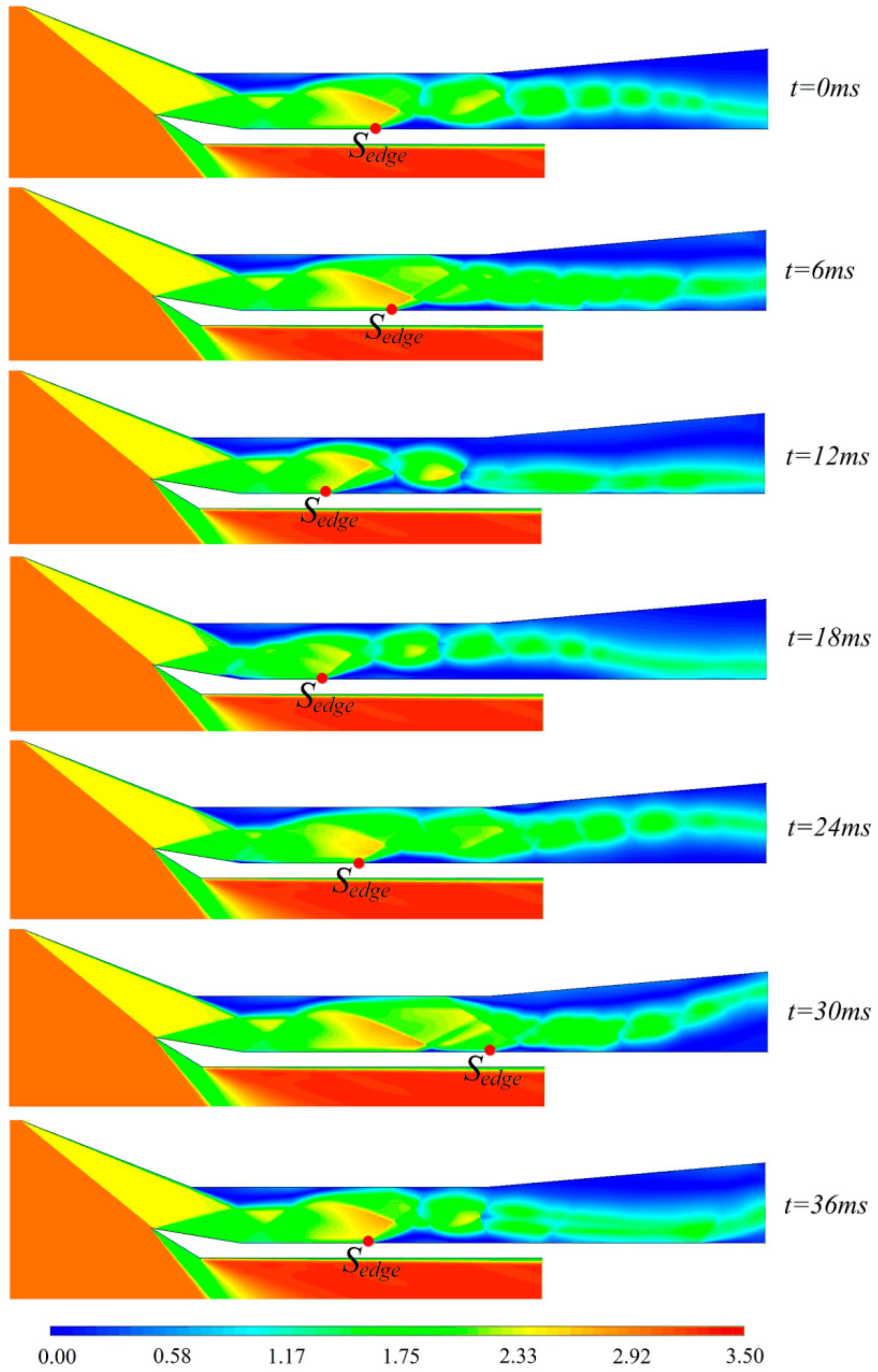
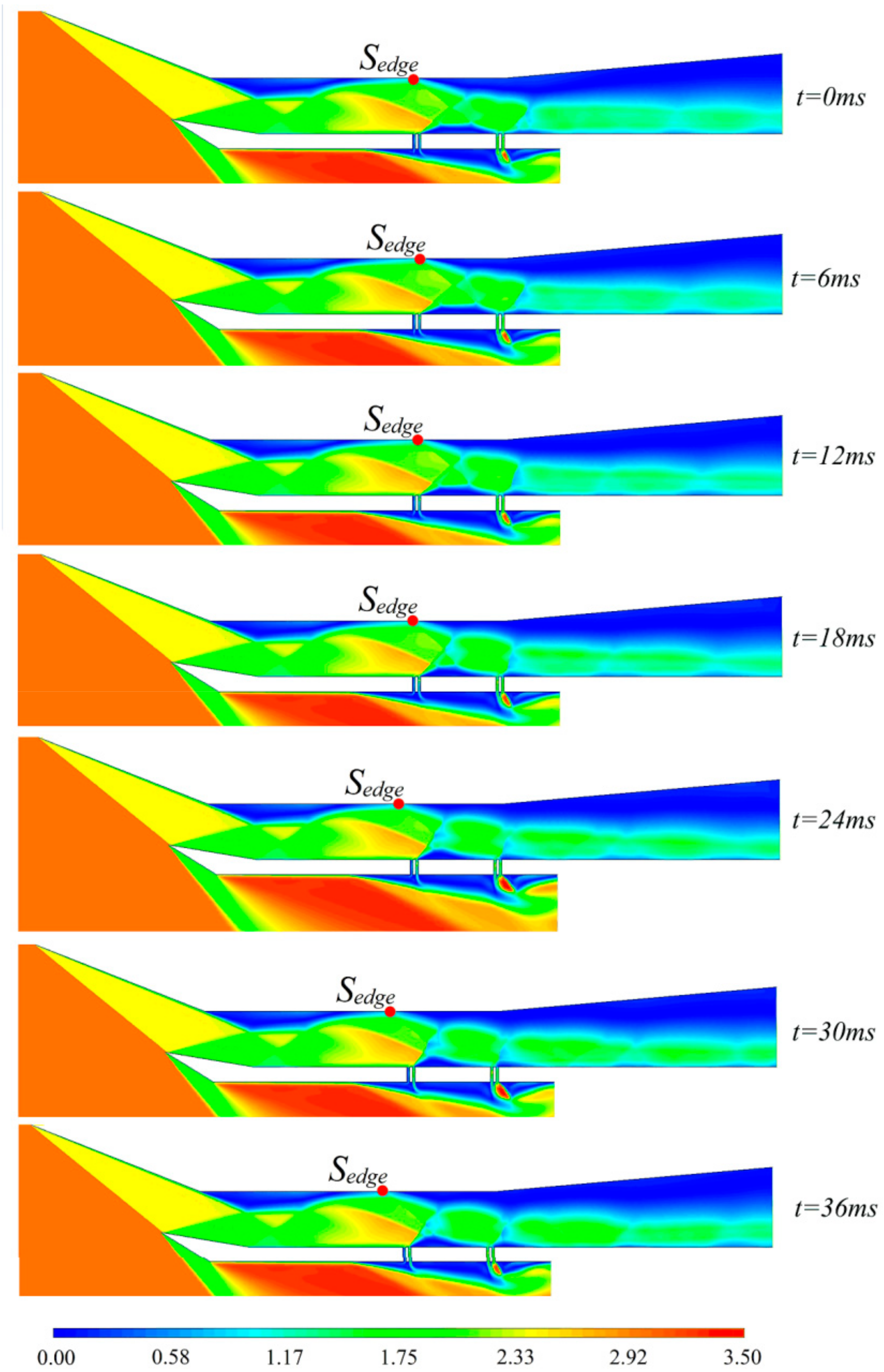
3.2.2. Analysis of Flow Field Characteristics and Flow Mechanism

The flow field variation laws of different calculation conditions are analyzed, and the suppression mechanism of the overflow on the shock wave oscillation is studied.

Figure 15 shows the flow field Mach number contour at 12 ms (starting at t = 0.200 s) of Model A. The shock wave system in the viscous flow field is very complex and produces three main separation zones in the inlet. The shock wave S₁ reflected from the lower lip of the inlet is incident on the upper wall to produce a separation zone R₁. The shock wave system interferes with the wall boundary layer to produce an obvious separation zone R₃ on the lower wall. In the expansion section of the inlet, the separation zone R₂ develops forward from the boundary layer due to the reverse pressure gradient. In the isolator, due to the compression of the incoming flow by the separation bubble in the R₃ region, a front shock wave S₃ is generated, which intersects with the shock wave S₄ on the upper wall, resulting in a bifurcated shock wave system S₅ and a backward-developed shock wave system S₆. It can be seen that the shock wave/boundary layer interaction is an important flow phenomenon in the inlet flow field, which has a complex impact on the shock wave system.

Figure 16 shows the motion state of the shock train in one cycle. From the perspective of the flow process, the shock train presents a dynamic state of change. The separation point moves from the back to the front within a certain period range. During the forward movement, the moving speeds of the upper and lower wall shocks wave do not remain constant. In the process of t = 12 ms~18 ms, the leading-edge point of the shock wave (S_edge in Figure 16) basically remains unchanged, and there is a certain pause process. This phenomenon is the same as that in reference [31], that is, under certain background waves, the shock wave movement is discontinuous. When the shock wave moves forward, the separation point on the upper wall is even connected to the separation area R₁, and the pressure also fluctuates due to the subsonic flow in the separation area. The shock wave moves forward to a specific position, the region’s volume after the shock wave increases and the pressure decreases, and the separated shock wave system moves backward again. Corresponding to Figure 12, when the leading edge of the shock wave moves forward and crosses sampling point 4, the pressure rises to produce a pulse, while after the separation shock wave moves backwards and crosses the position of sampling point 4, the pressure drops and then no longer changes. For sample point 8, the pressure continues to pulsate as it is constantly behind the separation shock wave. From the process in Figure 16, the shape and position of the shock wave system in the inlet, as well as the separation flow of the expansion section, have great changes in one cycle, and the shock wave has the characteristics of asymmetries and nonlinear movement.

When the overflow device is adopted, there are still separation zones, shock wave/boundary layer interference phenomena and complex shock wave systems in the flow field. From the local parameter distribution in Figure 17, the shock wave system is divided into two main parts. Between the two overflow gaps, the leading edge of the separation zone is constrained behind Gap_2. The front shock S₁ generated by the compression of the gas flow, intersects with the back oblique shock E₁ of the expansion zone on the upper wall and the oblique shock generated by the separation bubble on the upper wall to produce a typical “X” shaped shock S₂. A weak “X” type shock wave is generated behind the second overflow gap. The shock wave system did not cross the pre-overflow gap, and the difference between the internal and external pressures of the flow field was not large, so the flow velocity in Gap_2 was low. Gap_1 is located behind the shock wave system, and the flow pressure rises to about 10 times that of the incoming flow. Driven by the internal and external pressure difference, the flow in the gap has reached a choking state. The overflow from the isolator is blocked by the flow in the outflow field, resulting in the induced shock S₄. The pressure increases gradually in S₁, S₂ and S₃, and the local pressure in S₃ is significantly higher, which corresponds to the variation in the shock wave system.

Analyzing the Mach number change of the flow field in one cycle in Figure 18, compared with the state of Figure 16 without overflow, the shock wave system basically does not change within a cycle range. The shock front point, Sedge, on the upper wall changed slightly, which indicates that the shock position remained basically unchanged. The main oblique shock system is confined to the two overflow gaps on the lower wall. In the whole cycle, the flow velocity of the back overflow gap is high, but because the overflow gap is perpendicular to the flow direction of the mainstream, the flow is only about 3% of the inlet total flow. Since the leading edge of the shock wave system is limited behind the overflow gap Gap_2, the flow field before the sampling point 4 is not disturbed, and the pressure curve does not oscillate. Between sampling point 5 and sampling point 8, the oscillation amplitude of the shock wave decreases, and the oscillation amplitude of the pressure also decreases significantly.

According to the flow field characteristics, combined with the pressure curves of sampling points 4 and 8 in Figure 12 and Figure 13, when the shock wave moves forward, the pressure difference on both sides of the overflow gap increases sharply, and the airflow overflows the inlet. Theoretical analysis shows that the shock wave’s further forward movement will be “blocked”, thereby “locking” the shock wave at the overflow gap. The overflow process is fast. Through the overflow, the pressure in the area after the shock wave drops, and the shock wave moves backward. Correspondingly, the existence of the overflow gap also constrains the rapid backward movement of the shock wave. Therefore, under the action of the overflow gap, the shock wave oscillation process is weakened by constraining the forward and backward movement of the shock wave. The forward overflow gap Gap_2 in Model C is located at the leading edge of the shock wave system, and it has a good effect on the suppression of parameter oscillation under small overflow. In addition, the overflow gap of Model B is located behind the shock surface, which has a relatively weak inhibitory effect on shock oscillation. These are consistent with the results of the theoretical analysis.

4. Conclusions

Based on the theoretical method, this paper studies the influence law of the overflow on the flow field parameters in the shock train region. The flow field and its parameter change laws with the two overflow gap structures are numerically investigated and compared, and the following conclusions are drawn:

(1) The established shock wave dynamics model is used to calculate the steady-state flow field, which is consistent with the results of shock wave theory. The comparison with the reference example shows the feasibility of the modeling and calculation method in this paper.

(2) Based on the theoretical analysis of shock wave dynamics, when the overflow gap is used, the pressure oscillation amplitude of the flow field can be reduced to a certain extent, and both the rate of overflow and the gap position have an impact on the shock wave oscillation suppression. Increasing the rate of overflow and setting the overflow position in the shock surface area can improve the suppression effect of parameter oscillation.

(3) When there is no overflow gap, the separation shock wave has a wide range of fluctuations in the isolator and has the characteristics of nonlinear change. The frequency corresponding to the maximum amplitude point is 417 Hz, and there are multiple frequency points with large amplitudes in the range of 300 Hz~600 Hz.

(4) When the overflow gap is used, on the one hand, the amplitude of pressure pulsation caused by shock wave oscillation can be reduced. On the other hand, the frequency of shock self-excited oscillation increased significantly, and the oscillation frequency of the flow curves of Model B and Model C increased by more than 3 times compared with no overflow. The two models have obvious suppression of the oscillation process. The PL8 pressure amplitude is 53.86% and 30.56% of that without overflow, respectively, and the corresponding average overflow is within 3.6%.

(5) In Model C, the shock wave system is constrained between the front and back overflow gaps, which hinders the forward and backward movement of the shock wave and effectively suppresses the parameters fluctuation during the self-excited oscillation.

In general, the theoretical and numerical simulation results show that the overflow gap has a good effect on suppressing the self-excited oscillation of the supersonic flow field of the inlet shock wave system, and the rate of overflow is within a feasible range.

References

1. Matsuo, K.; Miyazato, Y.; Kim, H.D. Shock train and pseudo-shock phenomena in internal gas flows. Prog. Aerosp. Sci. 1999, 3, 33–100. [Google Scholar] [CrossRef]
2. Shapiro, A. The Dynamics and Thermodynamics of Compressible Fluid Flow; Wiley: Hoboken, NJ, USA, 1953; Volume 1. [Google Scholar]
3. Yu, J.; Li, J.; Wang, Q.; Zhang, X.; Zhang, S. Numerical and Experimental Study on the Duration of Nozzle Starting of the Reflected High-Enthalpy Shock Tunnel. Appl. Sci. 2022, 12, 2845. [Google Scholar] [CrossRef]
4. Hadjadj, A.; Dussauge, J.P. Shock Wave Boundary Layer Interaction. Shock Waves 2009, 19, 449–452. [Google Scholar] [CrossRef]
5. Humble, R.A.; Scarano, F.; Van Oudheusden, B.W. Unsteady aspects of an incident shock wave/turbulent boundary layer interaction. J. Fluid Mech. 2009, 635, 47–74. [Google Scholar] [CrossRef] [Green Version]
6. Wang, B. The Investigation into the Shock Wave/Boundary-Layer Interaction Flow Field Organization; National University of Defense Technology: Changsha, China, 2015. [Google Scholar]
7. Orton, G.F.; Scuderi, L.F.; Sanger, P.W.; Artus, J.; Laruelle, G.; Shkadov, L.H. Airbreathing hypersonic aircraft and transatmospheric vehicles. Prog. Astronaut. Aeronaut. 1997, 172, 297–372. [Google Scholar]
8. Kejing, X.; Juntao, C.; Nan, L.; Wen, B.; Daren, Y. Recent research progress on motion characteristics and flow mechanism of shock train in an isolator with background wave. J. Exp. Fluid Mech. 2019, 33, 31–42. [Google Scholar]
9. Meier, G.E.A.; Szumowski, A.P.; Selerowicz, W.C. Self-excited oscillations in internal transonic flows. Prog. Aerosp. Sci. 1990, 27, 145–200. [Google Scholar] [CrossRef]
10. Bruce, P.J.; Babinsky, H. Unsteady shock wave dynamics. J. Fluid Mech. 2008, 603, 463–473. [Google Scholar] [CrossRef] [Green Version]
11. Chakravarthy, R.V.K.; Nair, V.; Muruganandam, T.M.; Ghosh, S. Analytical and numerical study of normal shock response in a uniform duct. Phys. Fluids 2018, 30, 086–101. [Google Scholar] [CrossRef]
12. Takefumi, I.; Kazuyasu, M. Oscillation phenomena of pseudo-shock waves. Bull. JSME 1974, 17, 1278–1285. [Google Scholar]
13. Holger, B.; Harvey, J.K. Shock Wave Boundary-Layer Interactions; Cambridge University Press: Cambridge, UK, 2011. [Google Scholar]
14. Li, N.; Chang, J.; Yu, D.; Bao, W.; Song, Y. Mathematical model of shock-train path with complex background waves. J. Propuls. Power 2016, 33, 468–478. [Google Scholar] [CrossRef]
15. Hankey, W.L.; Shang, J.S. Analysis of Self-Excited Oscillations in Fluid Flow; AIAA: Reston, VA, USA, 1980; p. 1346. [Google Scholar]
16. Piponniau, S.; Dussauge, J.P.; Debieve, J.F.; Dupont, P. A simple model for low-frequency unsteadiness in shock-induced separation. J. Fluid Mech. 2009, 629, 87–108. [Google Scholar] [CrossRef]
17. Wagner, J.L.; Yuceil, K.B.; Valdivia, A.; Clemens, N.T.; Dolling, D.S. Experimental investigation of unstart in an inlet/isolator model in Mach 5 flow. AIAA J. 2009, 47, 1528–1542. [Google Scholar] [CrossRef]
18. Tan, H.J.; Sun, S.; Huang, H.X. Behavior of shock trains in a hypersonic inlet/isolator model with complex background waves. Exp. Fluids 2012, 53, 1647–1661. [Google Scholar] [CrossRef]
19. Tian, X.A.; Wang, C.P.; Cheng, K.M. Experimental investigation of dynamic characteristics of oblique shock train in Mach 5 flow. J. Propuls. Technol. 2014, 35, 1030–1039. [Google Scholar]
20. Lu, L.; Wang, Y.; Fan, X.Q.; Yan, G.W.; Meng, Z.W. Investigation of Shock-Train Forward Movement in Mixer of RBCC. J. Propuls. Technol. 2019, 40, 69–75. [Google Scholar]
21. Lv, H.; Wang, Z.; Chen, J.; Xu, L. The Influence of Boundary Layer Caused by Riblets on the Aircraft Surface. Appl. Sci. 2020, 10, 3686. [Google Scholar] [CrossRef]
22. Kim, J.; Park, Y.M.; Lee, J.; Kim, T.; Kim, M.; Lim, J.; Jee, S. Numerical Investigation of Jet Angle Effect on Airfoil Stall Control. Appl. Sci. 2019, 9, 2960. [Google Scholar] [CrossRef] [Green Version]
23. Weiss, A.; Olivier, H. Behaviour of a Shock Train under the Influence of Boundary-Layer Suction by a Normal Slot. Exp. Fluids 2012, 52, 273–287. [Google Scholar] [CrossRef]
24. Harloff, G.J.; Smith, G.E. On Supersonic Inlet Boundary Layer Bleed Flow; AIAA: Reston, VA, USA, 1995; p. 0038. [Google Scholar]
25. Soltani, M.R.; Daliri, A.; Younsi, J.S.; Farahani, M. Effects of bleed position on the stability of a supersonic inlet. J. Propuls. Power 2016, 32, 1153–1166. [Google Scholar] [CrossRef]
26. Chang, J.T.; Bao, W.; Cui, T.; Yu, D.R. Effect of suctions on maximum backpressure ratios of hypersonic inlets. J. Aerosp. Power 2008, 23, 505–509. [Google Scholar]
27. Ma, L.C. Study on the Effect of Suction Structure and Parameters on the Boundary Layer Oscillation Suction; Harbin Institute of Technology: Harbin, China, 2019. [Google Scholar]
28. Cravero, C.; Leutcha, P.J.; Marsano, D. Simulation and Modeling of Ported Shroud Effects on Radial Compressor Stage Stability Limits. Energies 2022, 15, 2571. [Google Scholar] [CrossRef]
29. Herrmann, D.; Siebe, F.; Gulhan, A. Pressure fluctuations (buzzing) and inlet performance of an airbreathing missile. J. Propuls. Power 2013, 29, 839–848. [Google Scholar] [CrossRef]
30. Huang, R.; Li, Z.F.; Nie, B.P.; Hong, Y.T.; Yang, J.M.; Wu, Y.C. Shock train oscillations in a two-dimensional inlet/isolator with suction. J. Propuls. Technol. 2020, 41, 767–777. [Google Scholar]
31. Reinartz, B.U.; Herrmann, C.D.; Ballmann, J.; Koschel, W.W. Aerodynamic performance analysis of a hypersonic inlet isolator using computation and experiment. J. Propuls. Power 2003, 19, 868–875. [Google Scholar] [CrossRef]
32. Liu, Z.; Wang, C.; Zhang, K.; Zhao, Z.; Xie, Z. Research on Computational Method of Supersonic Inlet/Isolator Internal Flow. Appl. Sci. 2021, 11, 9272. [Google Scholar] [CrossRef]
33. Pan, J.S.; Shan, P. Fundamentals of Aerodynamics; National Defense Industry Press: Beijing, China, 2011. [Google Scholar]
34. Zhao, R.; Yan, C. Evaluation of engineering turbulence models for complex supersonic flows. J. Beijing Univ. Aeronaut. Astronaut. 2011, 37, 202–205+215. [Google Scholar]
35. Wong, H.Y.W. Theoretical prediction of resonance in nozzle flows. J. Propuls. Power 2015, 21, 300–313. [Google Scholar] [CrossRef]
36. Xu, K.J.; Chang, J.T.; Zhou, W.X.; Yu, D. Mechanism and prediction for occurrence of shock-train sharp forward movement. AIAA J. 2016, 54, 1403–1412. [Google Scholar] [CrossRef]
Figure 1. Inlet geometric model.
Energies 15 03879 g001
Figure 2. Schematic of sampling points.
Energies 15 03879 g002
Figure 3. Shock wave motion calculation model.
Energies 15 03879 g003
Figure 4. Computing domain and mesh.
Energies 15 03879 g004
Figure 5. Comparison of wall pressure distribution Ma0 = 2.41. (a) Upper wall. (b) Lower wall.
Energies 15 03879 g005
Figure 6. Comparison between the calculated results and those in reference [31]. (a) Ma0 = 2.41. (b) Ma0 = 3.00.
Energies 15 03879 g006
Figure 7. Shock wave periodic motion process.
Energies 15 03879 g007
Figure 8. Parameters variation with the time under different ξ. (a) Export flow. (b) Shock position.
Energies 15 03879 g008
Figure 9. Parameter fluctuation with different positions when ξ = 6%. (a) Export flow. (b) Shock position.
Energies 15 03879 g009
Figure 10. Variation of flow over time. (a) Export flow. (b) Rate of overflow.
Energies 15 03879 g010
Figure 11. Spectrum analysis and comparison of different models.
Energies 15 03879 g011
Figure 12. Pressure change at sampling point 4. (a) Upper wall (b) Lower wall.
Energies 15 03879 g012
Figure 13. Pressure change at sampling point 8. (a) Upper wall (b) Lower wall.
Energies 15 03879 g013
Figure 14. Amplitude change at sampling point. (a) Upper wall. (b) Lower wall.
Energies 15 03879 g014
Figure 15. Mach number Isolines of Model A at t = 12 ms.
Energies 15 03879 g015
Figure 16. Mach number contour change process of Model A.
Energies 15 03879 g016
Figure 17. Isolines of Model C local parameters. (a) Mach number. (b) Pressure.
Energies 15 03879 g017
Figure 18. Mach number change process of Model C.
Energies 15 03879 g018