Towards Predictive Crude Oil Purchase: A Case Study in the USA and Europe

Abstract

Crude oil price volatility impacts the global economy in general, as well as the economies of Europe and the United States in particular; it is supremely difficult to describe its tendency precisely, hence it leads to a forecasting methodology. This study aims to use the autoregressive integrated moving average (ARIMA), and seasonal autoregressive integrated moving average (SARIMA) approaches to cope with this problem in the United States and Europe. The data was gathered from the U.S. Energy Information Administration and federal research economic data (FRED) from January 2017 to September 2021. Simultaneously, values from January 2017 to March 2021, with 51 observations accounting for 90% of the total samples, were employed for the training phase, and the rest were used for the testing phase. The forecast result also indicated that the root mean square error (RMSE) and mean absolute percentage error (MAPE) values, applied by ARIMA models in Europe and the United States, have higher accurate indicators than SARIMA models. As a result, the ARIMA model achieved the best accuracy in both Europe and the USA, with ${\mathrm{MAPE}}_{\mathrm{Europe}-\mathrm{ARIMA}}$ = 0.05, and ${\mathrm{MAPE}}_{\mathrm{USA}-\mathrm{ARIMA}}=0.05$. Based on these accuracy parameters, the forecasting models appear incredibly reliable; similarly, the study results might assist governing bodies in making significant decisions, thereby accelerating socio-economic development in the world’s two largest economies.

1. Introduction

Crude oil plays an essential role in global economic life. It has become increasingly important in the era of accelerating industrialization and modernization. Over recent years, crude oil has contributed significantly to the budgets of many countries worldwide, even more than the balance of international trade, contributing to countries’ budget revenues [1]. Crude oil prices have been closely observed, especially since the coronavirus disaster, and many investors seek oil price predictions for the upcoming period [2]. Oil pricing remains the largest share of energy for most estimated periods and will play a key role in meeting world energy needs [3] and crude oil pricing serves as a fundamental factor, taking over the investment picture in the long run [4]. More importantly, oil has been a critical variable in the valuation of economic growth [5].

With regard to classical forecasting methods, ARIMA and SARIMA models have been used successfully in plentiful applications such as oil price prediction [6,7,8,9]. The two models for our proposed experiments are considered supervised learning; hence, machine learning algorithms may be applied to create a model based on training data to make predictions or judgments without being explicitly programmed [10,11,12,13]. Machine learning is also known as predictive analytics when used to solve business challenges [14,15]. Mohammadi and Su [16] investigated the effectiveness of many autoregressive integrated moving average generalized autoregressive conditional heteroscedasticity (ARIMA-GARCH) models for modeling and predicting the volatility of weekly crude oil spot prices and the conditional mean in eleven international markets from 1 February 1997 to 10 March 2009. Nochai and Nochai [17] indicated the best ARIMA (1, 0, 1) for the forecast model of the palm oil price in Thailand. Ahmed and Shabri [18] indicated that ARIMA and GARCH techniques are the most efficient methods in predicting daily crude oil prices, with the study results also revealing that ARIMA is the best-fitted model compared with others; moreover, Wang et al. [19] proposed nonlinear grey model and linear ARIMA (NMGM-ARIMA) approaches to forecast the U.S. shale oil production using the quarterly dataset of 2003–2008 and 2008–2013. On the other hand, Tayib et al. [20] indicated that the most appropriate model for Malaysian crude palm oil production with the best optimal parameters of $\mathrm{SARIMA} \left(\mathrm{p},\mathrm{d},\mathrm{q}\right){\left(\mathrm{P},\mathrm{D},\mathrm{Q}\right)}_s$ is SARIMA (1, 0, 0)(0, 1, 1)₁₂, while Etuk, Amadi [21] employed SARIMA models to forecast the domestic crude oil production in Nigeria from January 2006 to August 2012. Ahmad, Abdul [22] used the SARIMA model to predict the crude palm oil and kernel palm production between June 2011 and May 2011 with the study results also showing that SARIMA is the most fitted model compared to other methods. Furthermore, Luo et al. [23] deployed SARIMA with a back propagation neural network (SARIMA-BP) hybrid model to forecast the international crude oil price from January 2002 to April 2006.

Hence, these helpful study results will provide valuable models and methods for deploying ARIMA and SARIMA algorithms in predicting oil prices in both the USA and European regions.

Other elements containing financial markets, economic development, the advent of new technology and events, on the other hand, also affect oil prices, promoting the crude oil market to surge significantly. Accordingly, forecasting crude oil prices is always a daunting task [24]; nonetheless, because crude oil is the world’s most important source of energy and governs most of the world’s economic activity, finding a promising forecasting technique for the oil price time series is far from outdated. Accurate prediction of oil prices sheds light on the decision-making of various areas such as commercial corporations and governing bodies [25]. Typically, the crude oil price changes significantly influencing the economic activities of the globe from many perspectives, although it has been mainly free to fluctuate with regard to the powers of need and supply [26]. Other elements such as financial markets, economic development, technological progress and unusual events also affect the crude oil price in several manners; additionally, accurate forecasting of crude oil prices is necessary to gain insight into the future development trends of the economy.

This paper aims to compare the changes in crude oil purchase prices and the results of the ARIMA and SARIMA models for crude oil purchase pricing forecasting in the United States and Europe from January 2017 to September 2021, to determine which model provides the most accurate forecast parameter for crude oil prices in the two regions. The input data used in the models contains 57 observations from January 2017 to September 2021, in Europe and the United States. This research also examines the differences between two models relying on the statistical accuracy parameter results such as the mean (M), root mean square error (RMSE), mean absolute percentage error (MAPE), mean absolute error (MAE), standard deviation (St Dev), skewness coefficient (Skew), minimum (Min) and maximum (Max). The collected results of these two models could illustrate the best-fitted models for predictive crude oil pricing in these two observed regions. In addition, this paper will help the USA and European governments catch the trends of oil price fluctuations, thereby ramping up economic development in the two regions and being valuable in forecasting recession in business cycles, and economic policies that could be enacted to weather an economic recession.

The following is the outline of the paper’s structure: Section 1 presents the paper’s introduction; Section 2 gives the area, and the SARIMA and ARIMA models and clarifies them clearly for understanding their use through this study; Section 3 demonstrates the data collection; Section 4 represents the results; Finally, Section 5 and Section 6 describe the discussions and conclusions.

2. Statistical Background

2.1. Autoregressive Integrated Moving Average (ARIMA) Model

The assumption of linear difference equations can be expanded to permit the forcing process {${\epsilon }_t$} to be stochastic. Hence, this type of linear stochastic difference equation underlies much of the assumption of time series econometrics. Specifically, the approach is critical for calculating time series models of the form:

$$y_t=\delta +{\varphi }_1{y}_{t-1}+\dots +{\varphi }_p{y}_{t-p}+{\epsilon }_t+{\theta }_1{\epsilon }_{t-1}+\dots +{\theta }_q{\epsilon }_{t-q}$$

(1)

Such models are autoregressive integrated moving average (ARIMA) time series models, so the series is supposed to be integrated of order d (written as I(d)), then the differenced stationary series can then be modeled as an ARIMA (p,d,q). In this case, the process that creates the series $y_t$ is called an autoregressive integrated moving average, and the model is ARIMA, represented as ARIMA (p,d,q).

2.2. Seasonal Autoregressive Integrated Moving Average (SARIMA) Model

An ARIMA model is considered a statistical time series forecasting method [27]. The SARIMA model is combined by seasonal autoregressive (SAR) [28], intergraded, and moving average (SMA) components. If the time series $y_t$ is demonstrated as SARIMA (p,d,q) × ${\left(P,D,Q\right)}_s$, it can be asserted as [29,30]:

$${\varphi }_p\left(B\right){\Phi }_P\left(B^s\right)W_t=\delta +{\theta }_q\left(B\right){\Theta }_Q\left(B^s\right){\epsilon }_t$$

(2)

where, p, d, and q are described in Equation (1). P, Q represents the order of seasonal autoregressive and seasonal moving average models, D describes the number of seasonal differencing, s indicates the length of the season (in monthly data s = 12), while ${\epsilon }_t$ shows the white noise value at period t. Here, B is a backward shift operator define as $B^s{y}_t=y_{t-s}$. $W_t={\nabla }^d\left(B\right){\nabla }_s^D\left(B\right)y_t$ is a stationary series since ${\nabla }^d\left(B\right)={\left(1-B\right)}^d$ and ${\nabla }_s^D\left(B\right)={\left(1-B^s\right)}^d$ are regular and seasonal stationarity transformation process, respectively. Therefore, Equation (2) can be extended mathematically as follows:

$${\varphi }_p\left(B\right){\Phi }_P\left(B^s\right){\left(1-B\right)}^d{\left(1-B^s\right)}^D{y}_t=\delta +{\theta }_q\left(B\right){\Theta }_Q\left(B^s\right){\epsilon }_t$$

(3)

The SARIMA components are defined as below:

$$\mathrm{nonseasonal} \mathrm{autoregression} \left(\mathrm{AR}\right): {\varphi }_p\left(B\right)=1-{\varphi }_{1}B-{\varphi }_2{B}^2-{\varphi }_3{B}^3-\dots -{\varphi }_p{B}^p$$

(4)

$$\mathrm{nonseasonal} \mathrm{moving} \mathrm{average} \left(\mathrm{MA}\right): {\theta }_q\left(B\right)=1-{\theta }_{1}B-{\theta }_2{B}^2-{\theta }_3{B}^3-\dots -{\theta }_q{B}^q$$

(5)

$$\mathrm{seasonal} \mathrm{autoregression} \left(\mathrm{SAR}\right): {\Phi }_P\left(B^s\right)=1-{\Phi }_1{B}^s-{\Phi }_2{B}^{2s}-{\Phi }_3{B}^{3s}-\dots -{\Phi }_P{B}^{Ps}$$

(6)

$$\mathrm{seasonal} \mathrm{moving} \mathrm{average} \left(\mathrm{SMA}\right): {\Theta }_Q\left(B^s\right)=1-{\Theta }_1{B}^s-{\Theta }_2{B}^{2s}-{\Theta }_3{B}^{3s}-\dots -{\Theta }_Q{B}^{Qs}$$

(7)

The d and D point out the order of the nonseasonal and seasonal differencing, and its values are usually not more than 1 and 2 in terms of the total of seasonal difference, respectively (i.e., 0 $\le$ d; D $\le$ 1) [31].

This study employs SARIMA with four stages as follows. In the first stage, study data is examined: stationarity or non-stationarity. In the second stage, the p-value and critical value cutoffs are determined by employing the test of augmented Dickey–Fuller. In the third stage, through the diagrams of the autocorrelation function (ACF) and partial autocorrelation function (PACF), the parameters of p, d, q, P, D, Q of the SARIMA model and are applied [28]. The seasonal MA and AR components, contingent on the ACF and PACF, reveal significant spikes at seasonal lags. The ACF and PACF are the most significant elements [32]. In the fourth stage, the parameter estimation of the normalized Bayesian information criterion (BIC) and Akaike information criterion is employed in order to investigate the SARIMA model [33]. The best model is when the indicator achieves optimal parameters such as AIC, BIC gain minimum values and exact indicators such as MAPE or RMSE, or the MAE approach at the minimum parameters.

The algorithm proposal (Figure 1) is designed to estimate the crude oil price and linear characteristics by researching seasonal time series data through ARIMA and SARIMA. Firstly, the database is preprocessed and tested via the statistical technique, and it is also split into training and testing phrases. Secondly, ARIMA and SARIMA algorithms are deployed to learn the training phrases and achieve optimal network indicators. Consequently, the two algorithm outputs are compared using metrics for calculating accuracy indicators, and the most appropriate estimation algorithm is found for the study.

2.3. Accuracy Measurement

Predicted results will be estimated and compared with the actual results to determine the predicted values accurately. Hence, standard metrics to evaluate the forecast accuracy include the mean absolute percentage error (MAPE), mean absolute error (MAE) and root mean square error (RMSE). The error metrics are explained as follows:

Let $y_t^f$ be the forecast of the dependent variable during the period of time t, and $y_t$ be the actual value, T is the number of observations. The accuracy indicators are represented as follows:

$$\mathrm{MAPE}=\frac{1}{\mathrm{T}}{\sum }_{t=1}^{\mathrm{T}}\frac{\left|y_t-y_t^f\right|}{\left|y_t\right|}$$

(8)

$$\mathrm{MAE}=\frac{{\sum }_{t=1}^{\mathrm{T}}\left|y_t-y_t^f\right|}{\mathrm{T}}$$

(9)

$$\mathrm{RMSE}=\sqrt{\frac{{\sum }_{t=1}^{\mathrm{T}}{\left(y_t-y_t^f\right)}^2}{\mathrm{T}}}$$

(10)

The model with lower values for these measurements would be better for predicting purposes. The MAE, RMSE approaches 0 indicating a strong model performance [34,35,36]; if MAPE ≤ 10%, it represents high accuracy forecasting; if 10% < MAPE ≤ 20%, we have good forecasting; if 20% < MAPE ≤ 50%, we obtain reasonable forecasting; if MAPE > 50%, it represents inaccurate forecasting; the accuracy measurements are employed to analyze the crude oil prices for this [37].

2.4. Min–Max Normalization

One of the most prevalent methods of data normalization is Min–Max normalization. Normalization is a method of scaling data from any range of values to between 0 and 1. This method requires us to determine the maximum (max) and minimum (min) values of data. The general formula for a Min–Max of [0, 1] is given as:

$$y=\frac{x-\min \left(x\right)}{\max \left(x\right)-\min \left(x\right)}$$

(11)

where x, y present for an original value of data and the normalized value of data; max(x) and min(x) indicate the highest and the lowest original value of data. Min–Max normalization has the advantage of annealing all values within a specific range.

3. Data Collection

The data for the monthly crude oil prices of the United States and Europe were obtained from the U.S. Energy Information Administration and federal research economic data (FRED) from January 2017 to September 2021, respectively. Thus, the dataset has 57 observations of crude oil pricing satisfying the principle of the Box–Jenkins technique for time series prediction [38]. Observations from January 2017 to March 2021 were deployed for the training set, and the values from April 2021 to September 2021 were used as the testing phase.

The data in Figure 2 indicates the seasonal series of crude oil prices in Europe and the USA by month, from January 2017 to September 2021, as follows: peak crude price season during the time period from May to October, due to the significant increase in oil demand in both regions, and the low season begins from March to June per annum. More importantly, the oil price fluctuations follow the same pattern throughout the period; nevertheless, the largest discrepancy between crude oil prices occurred in October 2018, suggesting that crude oil prices in Europe were approximately 16 USD ($) per barrel higher than those in the United States.

4. Result

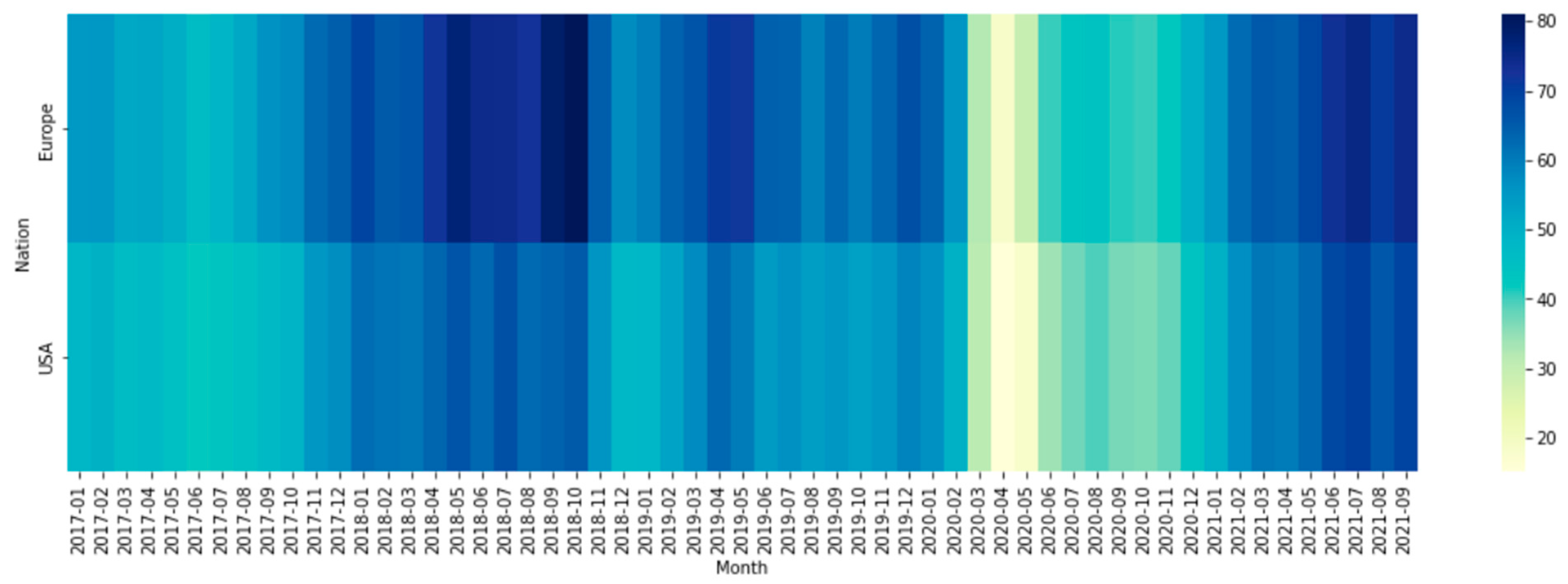
4.1. Descriptive Statistics

The parameters result in

Table 1. Descriptive statistics (Unit: USD).

Items	USA	Europe
Mean	52.28	59.41
Standard Deviation	11.86	13.03
Min	15.18	18.38
Max	70.12	81.03
Kurtosis	1.22	0.76
Skewness	−0.99	−0.86
Results of Dickey–Fuller Test
Test Statistic	−1.79	−1.78
p-value	0.38	0.39
Critical Value (1%)	−3.56	−3.56
Critical Value (5%)	−2.92	−2.92
Critical Value (10%)	−2.60	−2.60

describing descriptive statistics, containing the mean, minimum, and maximum values, kurtosis, skewness and standard deviation, were applied in the estimate to examine the characteristics of the data distribution. The mean represents a statistical indicator, which is the trend of the center in the data; the minimum and maximum values reveal the time series margin while the standard deviation is employed to estimate the data dispersion degree. According to the description of statistical results in Table 1, the standard deviations and the means of the two mentioned regions were $11.86 and $52.28 in the USA, $13.03 and $59.41 in Europe, respectively. A normal distribution’s skewness is nearly zero, and any symmetric data should have a skewness close to zero. Skewed left data is shown by negative skewness values, while skewed right data is indicated by positive skewness values [39,40]. Skewness coefficients were relatively low for data phrases; therefore, the values of the kurt and skew of the data fluctuating from −0.99 to 1.22 would be accepted for forecasting. Simultaneously, the crude oil purchase price employing the augmented Dickey–Fuller (ADF) test also points out that the observed data of crude oil price in the USA (with p-value = 0.38, test statistic = −1.79) and in Europe (with p-value = 0.39, test statistic = −1.78) have a unit root, indicating that these data are non-stationary. Moreover, when the time series data is non-stationary, it cannot be easily modeled with higher accuracy than the stationary data [41].

4.2. Application

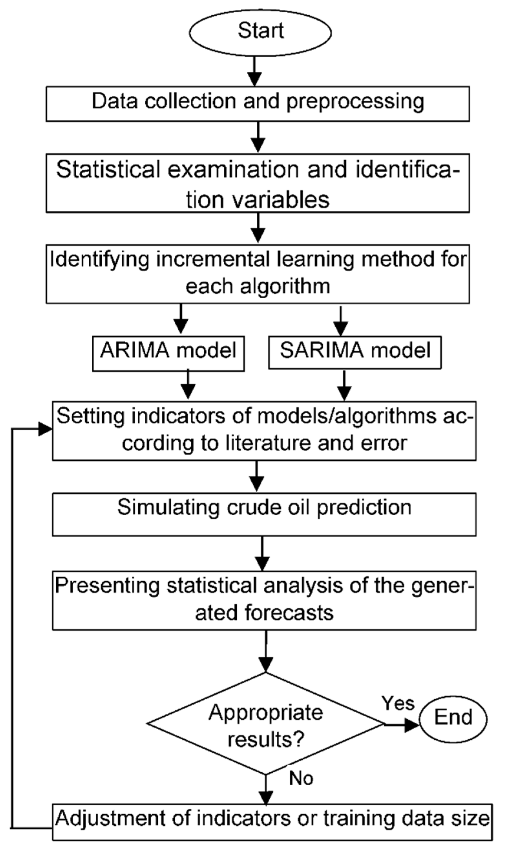
4.2.1. The Five Steps for This Experiment Determine the Optimal Predictive Models

The five steps for this experiment verify the optimal predictive models for forecasting the crude oil price prediction in the USA and Europe. Firstly, the crude oil price is normalized by deploying a Min–Max scaler, and secondly, the following four steps and the correlation plots of the ACF and PACF are conducted to examine the optimal parameters.

The calibration data in Figure 3 indicate that the crude oil time series in Europe and the USA witnessed the same trend tendency. As a result, these values decreased in April 2019 and reached their lowest points in March 2020, at around $31 and $32 per barrel, respectively. Therefore, these outputs can be considered a predictor of seasonal behavior patterns.

Decomposition is a strong tool for determining how time series data behaves. A time series can be divided into different components known as trend, observed, seasonal, and residual. The trend component shows a long-term shift in the data; the observed component denotes data changes that are not tied to a certain time frame but are typically linked to business cycles, while the seasonal component shows how the data fluctuates depending on the weather or the time of year. Therefore, the illustration of the crude oil price forecast aims to examine the optimal predictive model.

First of all, this study investigates the seasonality presence. The four-line diagrams in Figure 4 point out the decomposition of time series, consisting of trend, seasonality, observed and residual components, where it could be estimated that the lines are highly seasonal. At the same time, it is clear that a trend is not maintained throughout the line, also implying that the crude oil price in Europe is substantially greater than in the USA. More importantly, the crude oil price dramatically declined in both regions during the period from April 2020 to August 2020.

The correlation plots of the ACF and PACF (see Appendix A, Figure A1 and Figure A2) show that these plot oscillations are sinusoidal; moreover, these fluctuations also point out that the data are suitable with the SARIMA model to represent the crude oil price in Europe and the United States.

The standardized residual plots (see Appendix A, Figure A3a and Figure A4a) imply that the residuals are considered white noise, and that the histogram of the orange kernel density estimation (KDE) curve line is close to the actual distribution with the green N(0,1) curve line, so it also matches the description of its fundamental characteristics of the distribution standards. Additionally, the correlogram plots (see Appendix A, Figure A3c and Figure A4c) indicate that the residuals of the original data have a relatively low correlation with the lagged data of itself. It also reveals the autocorrelation trends of the United States and Europe are nearly consistent and do not surpass the interval between the z value of −0.25 and 0.25. Finally, the Q–Q plots (see Appendix A, Figure A3d and Figure A4d) demonstrate the distribution of the ordered residuals with blue spots staying on the red line, with a standard deviation equal to 1 and a mean equal to 0. In addition, the clusters of the residuals in both Europe and the USA are close to the straight line with the intercept −2; therefore, the linearity of the points proposes that the observed data are normally distributed in the USA and Europe. In summary, the obtained data are stable, the calculated findings are reliable, and can be used for analysis and estimated forecasting in both regions.

The data used for this study is big data that is statistically analyzed by month, so the simulation experiment has collected the optimal set of SARIMA and ARIMA parameter values with the smallest AIC. However, this study also evaluates the optimal model based on the MAPE parameters to determine the optimal model, so the output values in

Table 2. Akaike information criteria from several of the tested prediction models in Europe and the USA.

Europe						USA
ARIMA	AIC	MAPE	SARIMA	AIC	MAPE	ARIMA	AIC	MAPE	SARIMA	AIC	MAPE
(2,0,0)	−103.04	0.24	(2,1,0) × (0,1,1,12)	−63.55	0.24	(2,0,0)	−97.67	0.28	(2,1,0) × (0,1,1,12)	−56.06	0.33
(1,0,1)	−106.69	0.23	(0,1,1) × (0,1,1,12)	−63.28	0.25	(1,0,1)	−100.58	0.27	(0,1,1) × (0,1,1,12)	−55.91	0.34
(2,0,1)	−104.69	0.24	(2,1,0) × (2,1,0,12)	−62.59	0.24	(2,0,1)	−98.93	0.29	(0,1,2) × (0,1,1,12)	−54.61	0.33
(0,1,1)	−110.53	0.63	(2,1,0) × (0,1,2,12)	−62.53	0.23	(0,1,1)	−104.73	1.97	(2,1,1) × (0,1,1,12)	−54.59	0.30
(1,1,1)	−108.53	0.64	(2,1,0) × (1,1,1,12)	−62.45	0.24	(1,1,1)	−103.02	1.94	(0,1,2) × (0,1,1,12)	−54.43	0.39

witnessing the best suitable models for the Europe and USA crude oil price are SARIMA (2, 1, 0) × (1, 1, 1, 12) and SARIMA (2, 1, 1) × (0, 1, 1, 12), respectively, which are elected by relying on the minimum parameters of ${\mathrm{AIC}}_{\mathrm{Europe}}$ = −63.53 with the MAPE = 0.23, and ${\mathrm{AIC}}_{\mathrm{USA}}$ = −54.59 with MAPE = 0.30 in the training phrase, respectively. Moreover, the results point out the best appropriate models for Europe and USA crude oil price are ARIMA (1, 0, 1) and ARIMA (1, 0, 1), respectively, which are chosen by relying on the minimum parameters of ${\mathrm{AIC}}_{\mathrm{Europe}}$ = −106.69, ${ \mathrm{MAPE}}_{\mathrm{Europe}}$ = 0.23, and ${\mathrm{AIC}}_{\mathrm{USA}}$= −100.58, ${\mathrm{MAPE}}_{\mathrm{USA}}$= 0.27 in the training stage, respectively.

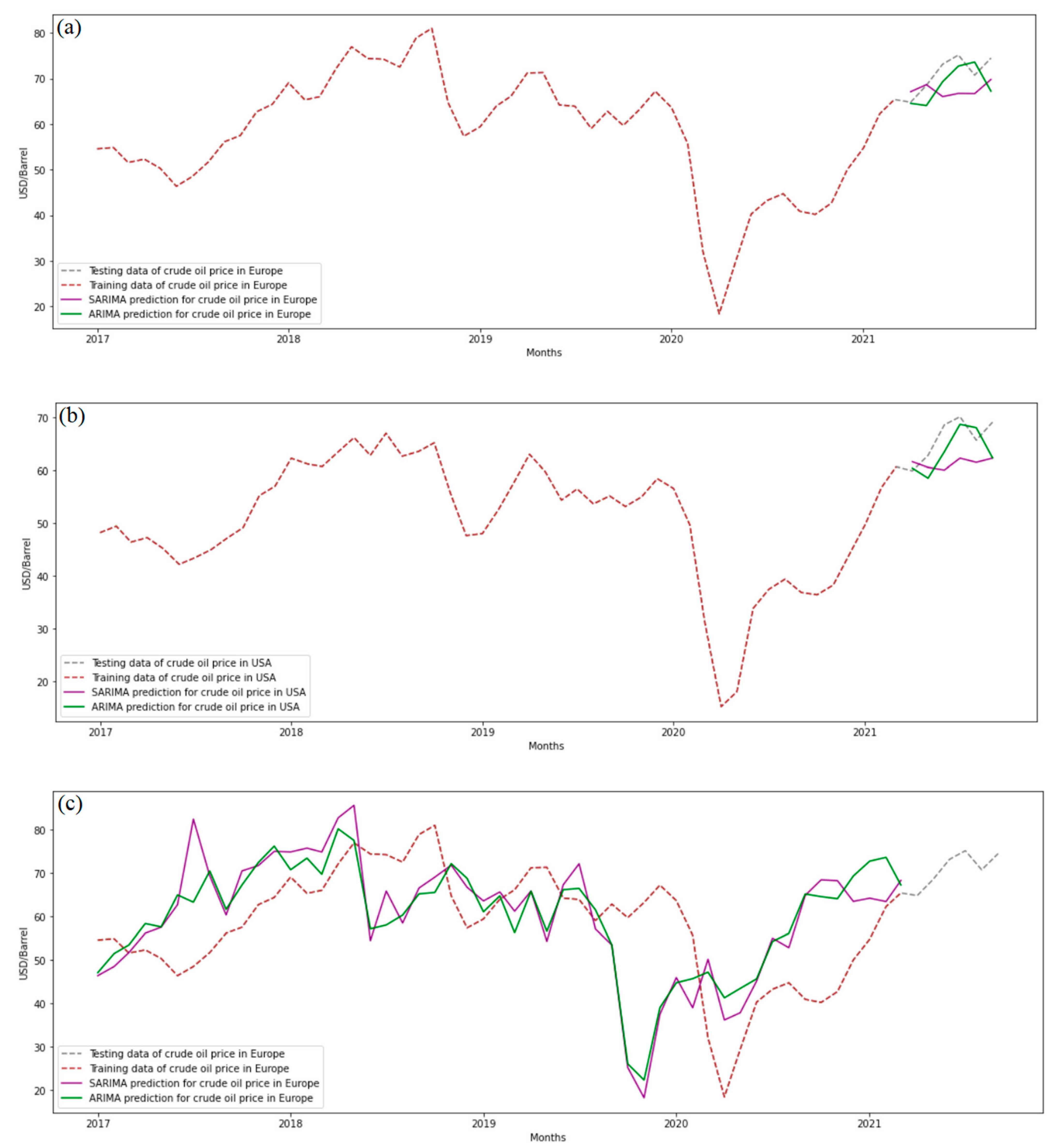
4.2.2. The Forecasting Crude Oil Price of the ARIMA and SARIMA Models

For the training and testing stages (in

Table 3. Accuracy parameters for crude oil forecast.

Parameter	ARIMA_Europe		SARIMA_Europe		ARIMA_USA		SARIMA_USA
	Testing	Training	Testing	Training	Testing	Training	Testing	Training
MAPE	0.05	0.24	0.06	0.24	0.05	0.27	0.09	0.30
MAE ($)	3.51	11.99	4.46	12.38	3.41	11.13	5.23	10.57
RMSE ($)	4.11	14.77	5.25	15.51	4.04	13.98	5.86	14.04

), the MAPE of two models in the crude oil prices ranges from 0.05 to 0.30. In the same way, the MAE indicators range from $3.41 to $12.38. Additionally, the values of the RMSE are simulated variations from $4.04 to $15.60. The experimental results for each model show that ARIMA and SARIMA lines for the testing stage are quite fitted to the actual lines, indicated in Figure 5a,b with ${\mathrm{MAPE}}_{\mathrm{EU}-\mathrm{SARIMA}}$ = 0.06, ${\mathrm{MAE}}_{\mathrm{Europe}-\mathrm{SARIMA}}$ = $4.46, ${\mathrm{RMSE}}_{\mathrm{Europe}-\mathrm{SARIMA}}$ = $5.25, ${\mathrm{MAPE}}_{\mathrm{USA}-\mathrm{SARIMA}}$ = 0.09, ${\mathrm{MAE}}_{\mathrm{USA}-\mathrm{SARIMA}}$ = $5.23, ${\mathrm{RMSE}}_{\mathrm{USA}-\mathrm{SARIMA}}$ = $5.86, respectively. At the same time, the highest accuracy parameters for the forecast are found in ARIMA models with ${\mathrm{MAPE}}_{\mathrm{Europe}-\mathrm{ARIMA}}$ = 0.05, and ${\mathrm{MAPE}}_{\mathrm{USA}-\mathrm{ARIMA}}=0.05$, and the lowest ones are in SARIMA models with ${\mathrm{MAPE}}_{\mathrm{Europe}-\mathrm{SARIMA}}$ = 0.06, and ${\mathrm{MAPE}}_{\mathrm{USA}-\mathrm{SARIMA}}=0.09$.

The lines from Figure 5c,d for the training phase prove that the forecast values created by the ARIMA models are very close to the actual lines (brown line) of crude oil prices in Europe and the USA. The parameters of MAPE, MAE, and RMSE (in Table 3) of crude oil price in Europe and the USA are ${\mathrm{MAPE}}_{\mathrm{Europe}-\mathrm{SARIMA}}$ = 0.24, ${\mathrm{MAE}}_{\mathrm{Europe}-\mathrm{SARIMA}}$ = $12.38, ${\mathrm{RMSE}}_{\mathrm{Europe}-\mathrm{SARIMA}}$ = $15.51, ${\mathrm{MAPE}}_{\mathrm{USA}-\mathrm{SARIMA}}$ = 0.30, ${\mathrm{MAE}}_{\mathrm{USA}-\mathrm{SARIMA}}$ = $10.57, ${\mathrm{RMSE}}_{\mathrm{USA}-\mathrm{SARIMA}}$ = $14.04. Meanwhile, the green lines of ARIMA are not fitted with the actual lines, so the time series value of these observations for the forecast of natural phenomena is moderately acceptable. Furthermore, the diagrams show that the forecast lines generated by the ARIMA models are very close to the actual lines of crude oil prices in Europe and the USA. Meanwhile, the forecast values generated by the ARIMA models are also relatively close to the actual values of crude oil prices in Europe and the USA, with ${\mathrm{MAPE}}_{\mathrm{Europe}-\mathrm{ARIMA}}$ = 0.24, ${\mathrm{MAE}}_{\mathrm{Europe}-\mathrm{ARIMA}}$ = $11.99, ${ \mathrm{RMSE}}_{\mathrm{Europe}-\mathrm{ARIMA}}$ = $14.77,${ \mathrm{MAPE}}_{\mathrm{USA}-\mathrm{ARIMA}}$ = 0.27, ${ \mathrm{MAE}}_{\mathrm{USA}-\mathrm{ARIMA}}$ = $11.13, ${\mathrm{RMSE}}_{\mathrm{USA}-\mathrm{ARIMA}}$ = $13.98. Therefore, the crude oil price in both mentioned regions will be predicted by ARIMA models more efficiently than by SARIMA techniques.

5. Discussion

In this study, employing ARIMA and SARIMA models predicted crude oil purchases of Europe and the United States, based on the monthly collected data for 5 years. Testing phases indicated that MAPE, MAE, and RMSE values of SARIMA models in Europe were higher than those of ARIMA models by 0.01, $0.95 and $1.14, respectively. When it came to the testing phase in the USA, the MAPE parameters generated by SARIMA techniques were higher than 0.01, compared with ARIMA models. As a result of these findings, the ARIMA model has shown higher forecast results for crude oil prices in Europe and the USA than the SARIMA model. Similarly, these findings can be used as reference data by governments to estimate crude oil price cycles and implement suitable policies in response to changes in crude oil prices.

Many recent crude oil price studies are related to SARIMA models. Manigandan et al. [42] indicated that researchers could attain the best prediction performance with a MAPE measure of roughly 9%, which is higher than this study’s MAPE values. As far as the research of Blázquez-García et al. [43] is concerned, their study witnessed accuracy indicators RMSE = 0.8, MAPE = 7.69, which employed the SARIMA model to forecast energy consumption. Therefore, the results attain a 1.69% lower accuracy than this study’s outputs with ${\mathrm{MAPE}}_{\mathrm{EU}-\mathrm{SARIMA}}$ = 0.06, but it represented 1.31% greater performance than ${\mathrm{MAPE}}_{\mathrm{USA}-\mathrm{SARIMA}}$ = 0.09. Another result from Tayib, Nor [20] showed an accuracy parameter MAE = 4.306 in the United States’ predicting crude oil prices, being much higher than this study’s accuracy value with MAE = 4.04 in the USA’s forecasting of crude oil prices.

However, some studies have deployed SARIMA models with daily data to predict crude oil prices, while Li et al. [44] employed improved CEEMDAN and ridge-regression-based predictors to predict daily crude oil prices. Therefore, these results of the ARIMA models’ MAPE values ranging from 0.02 to 0.04 outperform this study’s ARIMA algorithms in Europe and the USA. Furthermore, these results reveal that the RMSE index of these two mentioned studies is also smaller than the RMSE value of this study. Consequently, although the ARIMA and SARIMA models were considered the most classical methods, the models deployed for the time series data perform comparably to deep learning methods, including the long short-term memory network (LSTM) and convolutional neural network (CNN). For example, He et al. [45] employed SARIMA and deep learning methods, including LSTM and CNN, tested for forecasting Macao daily tourist arrivals, and according to their findings, the MAPE of the SARIMA model 0.09 is remarkably similar to the MAPE of the SARIMA–CNN–LSTM model 0.09. Therefore, these outputs have shown approximately the same accuracy level of this study’s SARIMA model in predicting crude oil prices in the U.S., but to a lesser extent in the European case study. Moreover, the ADF test result of Manigandan et al. [42] showed that the variable of natural gas plant liquids (NGPL) is significant at 5%. At the same time, the MAPE, and RMSE values are equal to 1636.48 and 69.45, which is higher than this study’s results.

Despite the fact that crude oil price forecasting involves seasonal volatility and varying levels of complexity, using these two models in three different configurations yielded results with high reliability. As a result, it could be used to forecast crude oil purchase pricing for other countries throughout the world. Besides, with the current circumstances of world crude oil volatility, further developing ARIMA and SARIMA techniques with multiple linear regression models could be employed in modeling crude oil prices in future research, assisting in enhancing a more accurate prediction level.

6. Conclusions

This paper examines the change in crude oil prices in both Europe and the USA. Relying on monthly data from January 2017 to September 2021, the study applies two models of ARIMA and SARIMA for predicting crude oil purchase prices. Additionally, three commonly used statistical factors were used to compare the predicted and observed values: MAPE, RMSE, and MAE parameters. As a result, both ARIMA and SARIMA attain high accuracy parameters; however, the ARIMA model received slightly greater accuracy parameters than the SARIMA algorithm for predicting crude oil prices in the United States and Europe. Furthermore, oil price changes follow a consistent trend over time; nonetheless, the highest disparity between crude oil prices occurred in October 2018, implying that crude oil prices in Europe were around $16 per barrel higher than those in the USA. Aside from these aforementioned research results, forthcoming studies can deploy ARIMA and SARIMA algorithms to anticipate crude oil prices in other countries.

The application domains and approaches discussed in this paper give readers a broad picture of the field’s current state of the art scenario. Potential researchers, in particular, could take advantage of the reported status quo to start new and innovative research projects. Furthermore, this study could be a significant step for the energy economic areas similar to other economic fields that aim to merge more transparent economic-driven models, including ARIMA and SARIMA algorithms. Likewise, this study concludes that machine learning models play a significant role in the decision-making process for determining the influences of crude oil price variation in the USA and Europe. Consequently, with the current state of world crude oil volatility, future studies can apply multiple linear regression with these techniques to estimate the potential elements impacted upon with energy price variations.

References

1. Alekhina, V.; Yoshino, N. Impact of World Oil Prices on an Energy Exporting Economy Including Monetary Policy; ADBI Working Paper No. 828; Asian Development Bank Institute (ADBI): Tokyo, Japan, 2018. [Google Scholar]
2. Erb, C.B.; Harvey, C.R. The strategic and tactical value of commodity futures. Financ. Anal. J. 2006, 62, 69–97. [Google Scholar] [CrossRef]
3. Shafiee, S.; Topal, E. When will fossil fuel reserves be diminished? Energy Policy 2009, 37, 181–189. [Google Scholar] [CrossRef]
4. Mensi, W.; Hammoudeh, S.; Shahzad, S.J.H.; Shahbaz, M. Modeling systemic risk and dependence structure between oil and stock markets using a variational mode decomposition-based copula method. J. Bank. Financ. 2017, 75, 258–279. [Google Scholar] [CrossRef]
5. Squalli, J. Electricity consumption and economic growth: Bounds and causality analyses of OPEC members. Energy Econ. 2007, 29, 1192–1205. [Google Scholar] [CrossRef]
6. Ghoddusi, H.; Creamer, G.G.; Rafizadeh, N. Machine learning in energy economics and finance: A review. Energy Econ. 2019, 81, 709–727. [Google Scholar] [CrossRef]
7. Ekechukwu, G.K.; Falode, O.; Orodu, O.D. Improved method for the estimation of minimum miscibility pressure for pure and impure co2–crude oil systems using Gaussian process machine learning approach. J. Energy Resour. Technol. 2020, 142, 123003. [Google Scholar] [CrossRef]
8. Abdullah, S.N.B. Machine Learning Approach for Crude Oil Price Prediction. Ph.D. Thesis, The University of Manchester, Manchester, UK, 2014. [Google Scholar]
9. Herrera, G.P.; Constantino, M.; Tabak, B.M.; Pistori, H.; Su, J.-J.; Naranpanawa, A. Data on forecasting energy prices using machine learning. Data Brief 2019, 25, 104122. [Google Scholar] [CrossRef]
10. James, S.C.; Zhang, Y.; O’Donncha, F. A machine learning framework to forecast wave conditions. Coast. Eng. 2018, 137, 1–10. [Google Scholar] [CrossRef] [Green Version]
11. Gao, S.; Lei, Y. A new approach for crude oil price prediction based on stream learning. Geosci. Front. 2017, 8, 183–187. [Google Scholar] [CrossRef] [Green Version]
12. Lippi, M.; Bertini, M.; Frasconi, P. Short-term traffic flow forecasting: An experimental comparison of time-series analysis and supervised learning. IEEE Trans. Intell. Transp. Syst. 2013, 14, 871–882. [Google Scholar] [CrossRef]
13. Ryoo, B.; Ashtab, M. Predictive capabilities of supervised learning models compare with time series models in forecasting construction hiring. EPiC Ser. Built Environ. 2021, 2, 117–126. [Google Scholar] [CrossRef]
14. Janiesch, C.; Zschech, P.; Heinrich, K. Machine learning and deep learning. Electron. Mark. 2021, 31, 685–695. [Google Scholar] [CrossRef]
15. Kelleher, J.D.; Mac Namee, B.; D’arcy, A. Fundamentals of Machine Learning for Predictive Data Analytics: Algorithms, Worked Examples, and Case Studies; MIT Press: Cambridge, MA, USA, 2020. [Google Scholar]
16. Mohammadi, H.; Su, L. International evidence on crude oil price dynamics: Applications of ARIMA-GARCH models. Energy Econ. 2010, 32, 1001–1008. [Google Scholar] [CrossRef]
17. Nochai, R.; Nochai, T. ARIMA model for forecasting oil palm price. In Proceedings of the 2nd IMT-GT Regional Conference on Mathematics, Statistics and Applications, Penang, Malaysia, 13–15 June 2006; pp. 13–15. [Google Scholar]
18. Ahmed, R.A.; Shabri, A.B. Daily crude oil price forecasting model using ARIMA, generalized autoregressive conditional heteroscedastic and support vector machines. Am. J. Appl. Sci. 2014, 11, 425. [Google Scholar] [CrossRef]
19. Wang, Y.; Wu, C.; Yang, L. Oil price shocks and agricultural commodity prices. Energy Econ. 2014, 44, 22–35. [Google Scholar] [CrossRef]
20. Tayib, S.A.M.; Nor, S.R.M.; Norrulashikin, S.M. Forecasting on the crude palm oil production in Malaysia using SARIMA Model. J. Phys. Conf. Ser. 2021, 1988, 012106. [Google Scholar] [CrossRef]
21. Etuk, E.H.; Amadi, E.H. Multiplicative SARIMA modelling of Nigerian monthly crude oil domestic production. J. Appl. Math. Bioinform. 2013, 3, 103. [Google Scholar]
22. Ahmad, S.; Latif, H.A. Forecasting on the crude palm oil and kernel palm production: Seasonal ARIMA approach. In Proceedings of the 2011 IEEE Colloquium on Humanities, Science and Engineering, Penang, Malaysia, 5–6 December 2011; pp. 939–944. [Google Scholar] [CrossRef]
23. Luo, H.; Liu, X.; Wang, S. Based on SARIMA-BP hybrid model and SSVM model of international crude oil price prediction research. ANZIAM J. 2016, 58, E143. [Google Scholar] [CrossRef] [Green Version]
24. Zhao, Y.; Li, J.; Yu, L. A deep learning ensemble approach for crude oil price forecasting. Energy Econ. 2017, 66, 9–16. [Google Scholar] [CrossRef]
25. Wachtmeister, H.; Henke, P.; Höök, M. Oil projections in retrospect: Revisions, accuracy and current uncertainty. Appl. Energy 2018, 220, 138–153. [Google Scholar] [CrossRef]
26. Baumeister, C.; Kilian, L. Forty years of oil price fluctuations: Why the price of oil may still surprise us. J. Econ. Perspect. 2016, 30, 139–160. [Google Scholar] [CrossRef] [Green Version]
27. Box, G.E.P.; Jenkins, G.M.; Reinsel, G.C.; Ljung, G.M. Time Series Analysis: Forecasting and Control, 5th ed.; John Wiley & Sons: Hoboken, NJ, USA, 2015. [Google Scholar]
28. Khanarsa, P.; Sinapiromsaran, K. Automatic SARIMA order identification convolutional neural network. Int. J. Mach. Learn. Comput. 2020, 10, 662–668. [Google Scholar] [CrossRef]
29. Aburto, L.; Weber, R. Improved supply chain management based on hybrid demand forecasts. Appl. Soft. Comput. 2007, 7, 136–144. [Google Scholar] [CrossRef]
30. Cools, M.; Moons, E.; Wets, G. Investigating the variability in daily traffic counts through use of ARIMAX and SARIMAX models: Assessing the effect of holidays on two site locations. Transp. Res. Rec. 2009, 2136, 57–66. [Google Scholar] [CrossRef] [Green Version]
31. Farsi, M.; Hosahalli, D.; Manjunatha, B.R.; Gad, I.; Atlam, E.-S.; Ahmed, A.; Elmarhomy, G.; Elmarhoumy, M.; Ghoneim, O.A. Parallel genetic algorithms for optimizing the SARIMA model for better forecasting of the NCDC weather data. Alex. Eng. J. 2021, 60, 1299–1316. [Google Scholar] [CrossRef]
32. Shumway, R.H.; Stoffer, D.S.; Stoffer, D.S. Time Series Analysis and Its Applications; Springer: New York, NY, USA, 2000; Volume 3. [Google Scholar]
33. Puthran, D.; Shivaprasad, H.C.; Kumar, K.K.; Manjunath, M. Comparing SARIMA and Holt-Winters’ forecasting accuracy with respect to Indian motorcycle industry. Trans. Eng. Sci. 2014, 2, 25–28. [Google Scholar]
34. Chicco, D.; Warrens, M.J.; Jurman, G. The coefficient of determination R-squared is more informative than SMAPE, MAE, MAPE, MSE and RMSE in regression analysis evaluation. PeerJ Comput. Sci. 2021, 7, e623. [Google Scholar] [CrossRef]
35. Obite, C.P.; Chukwu, A.; Bartholomew, D.C.; Nwosu, U.I.; Esiaba, G.E. Classical and machine learning modeling of crude oil production in Nigeria: Identification of an eminent model for application. Energy Rep. 2021, 7, 3497–3505. [Google Scholar] [CrossRef]
36. Ajumi, O.; Kaushik, A. Exchange rates prediction via deep learning and machine learning: A literature survey on currency forecasting. Int. J. Sci. Res. 2017, 7, ART20193849. [Google Scholar]
37. Lewis, C. International and Business Forecasting Methods; Butterworths: London, UK, 1982. [Google Scholar]
38. Chatfield, C. The Analysis of Time Series: An Introduction; Chapman and Hall/CRC: Boca Raton, FL, USA, 2003. [Google Scholar]
39. Sahu, S.K.; Dey, D.K.; Branco, M.D. A new class of multivariate skew distributions with applications to Bayesian regression models. Can. J. Stat. 2003, 31, 129–150. [Google Scholar] [CrossRef] [Green Version]
40. Brys, G.; Hubert, M.; Struyf, A. A robust measure of skewness. J. Comput. Graph. Stat. 2004, 13, 996–1017. [Google Scholar] [CrossRef]
41. Aiello, M.; Yang, Y.; Zou, Y.; Zhang, L.J. (Eds.) Artificial Intelligence and Mobile Services—AIMS; Springer International Publishing: New York, NY, USA, 2018. [Google Scholar]
42. Manigandan, P.; Alam, M.D.S.; Alharthi, M.; Khan, U.; Alagirisamy, K.; Pachiyappan, D.; Rehman, A. Forecasting natural gas production and consumption in United States-Evidence from SARIMA and SARIMAX models. Energies 2021, 14, 6021. [Google Scholar] [CrossRef]
43. Blázquez-García, A.; Conde, A.; Milo, A.; Sánchez, R.; Barrio, I. Short-term office building elevator energy consumption forecast using SARIMA. J. Build. Perform. Simul. 2019, 13, 69–78. [Google Scholar] [CrossRef]
44. Li, T.; Zhou, Y.; Li, X.; Wu, J.; He, T. Forecasting daily crude oil prices using improved CEEMDAN and ridge regression-based predictors. Energies 2019, 12, 3603. [Google Scholar] [CrossRef] [Green Version]
45. He, K.; Ji, L.; Wu, C.W.D.; Tso, K.F.G. Using SARIMA–CNN–LSTM approach to forecast daily tourism demand. J. Hosp. Tour. Manag. 2021, 49, 25–33. [Google Scholar] [CrossRef]
Figure 1. The procedure followed in this study’s experimental steps.
Energies 15 04003 g001
Figure 2. Monthly crude oil price in Europe and the USA from 2017 to 2021.
Energies 15 04003 g002
Figure 3. (a) Calibration vector of the monthly price of crude oil time series; (b) Calibration vector of the transformed monthly price of crude oil time series using Min–Max scaler.
Energies 15 04003 g003
Figure 4. The calibrating vector decomposition of the crude oil price time series.
Energies 15 04003 g004
Figure 5. The actual and forecasted crude oil price relying on ARIMA and SARIMA models for testing data in: (a) Europe; (b) the USA, and for training data in; (c) Europe; (d) the USA.
Energies 15 04003 g005aEnergies 15 04003 g005b