Parametric Transient Stability Constrained Optimal Power Flow Solved by Polynomial Approximation Based on the Stochastic Collocation Method

Abstract

To better respond to the impact of power system-uncertain parameters on transient stability, a novel model named the parametric transient stability constrained optimal power flow (parametric TSCOPF) is proposed. It seeks the optimal control scheme of transient stability constrained optimal power flow (TSCOPF) expressed by the function of uncertain parameters in power systems. The key difficulty to solve this model lies in that the relationship between the parametric TSCOPF solution and uncertain parameters is implicit, which is hard to derive generally. To this end, this paper approximates the optimal solution of parametric TSCOPF by polynomial expressions of uncertain parameters based on the stochastic collocation method. First, the parametric TSCOPF model includes both uncertain parameters and transient stability constraints, in which the transient stability constraint is constructed as a set of polynomial expressions using the SCM. Then, to derive the relationship between the parametric TSCOPF solution and uncertain parameters, the SCM is applied to the parametric Karush–Kuhn–Tucker (KKT) conditions of the parametric TSCOPF model, so that the optimal solution of the parametric TSCOPF is approximated by using polynomial expressions with respect to uncertain parameters. The proposed parametric TSCOPF model has been tested on a 3-machine, 9-bus system, and the IEEE 145-bus system, which verifies the effectiveness of the proposed method.

1. Introduction

The transient stability constrained optimal power flow (TSCOPF) [1,2,3,4,5] is an efficient tool to reconcile the requirements of economic operation and dynamic security in power systems, and the model of TSCOPF problem has been generally addressed as a deterministic optimization problem. However, renewable resources and nodal loads are uncertain factors in power systems, which have significant influence on the solution of deterministic TSCOPF. So it is necessary to consider the effect of these uncertain parameters in the TSCOPF problem, and implement control schemes to respond to the fluctuations of uncertain factors in power systems.

According to the manners of parameter uncertainty quantification and optimization model construction, there are two commonly used methods of solving optimization problems considering uncertain parameters, i.e., probabilistic optimization [6,7,8] and robust optimization [9,10]. Probabilistic optimization assumes that the uncertain parameters obey a certain determined probability distribution. It minimizes the expectation of generation cost, etc. as the objective function to build a stochastic probabilistic model satisfying a certain probability level constraints. This approach has been used in problems such as optimal siting and sizing of distributed generators [11], security-constrained unit commitment [12,13,14,15] and reserve dispatch with uncertain wind power output [16,17,18]. It has been shown that the strategy derived from probabilistic programming can optimize the expectations of the objective function under uncertainty. However, probabilistic optimization modeling requires the knowledge of complete information about the probability distribution of uncertain parameters. Robust optimization is widely used because it does not need to know the information of probability distribution of uncertain parameters. Robust optimization limits the value of all uncertain parameters within their variation range, and transforms the problem into a deterministic optimization problem to cater to the needs of all extreme scenarios. Robust optimization has been widely used to deal with uncertain parameters in economic dispatch [19,20,21,22], security-constrained unit commitment [23], and cooperative energy and reserve scheduling for multi-microgrids [24]. However, although robust optimization can effectively deal with uncertain parameters, the optimization results are often very conservative due to its neglection of the distribution information of uncertain parameters.

In this paper, a novel approach named parametric optimization is proposed. In the model of the parametric optimization, uncertain parameters are treated as independent variables which vary freely in their range, and the system variables and control parameters are treated as dependent variables of uncertain parameters. So the parametric optimization seeks a solution that characterize the quantitive relationship between the parametric optimization solution and uncertain parameters.

The difficulty of solving the well-known TSCOPF is that the transient equality constraint is a set of differential algebraic equations (DAEs) which are hard to be dealt with in the optimization model. For the parameteric TSCOPF (Pa-TSCOPF), this difficulty will be even more serious because the uncertain parameters are free to change in the optimization model. Therefore, to obtain the parametric solution, the relationship between system variables (containing both state and algebraic variables) in the transient process and parameters (containing both uncertain and control parameters) needs to be reformulated, thus the DAEs can be eliminated from the optimization model. There are three kinds of ways to solve this problem: (1) The Monte Carlo method [25] is a straightforward method to analyze the statistical characteristic of the transient variables. However, the dynamic models of power systems have the characteristics of high dimensionality and strong nonlinearity; thus this method is time-consuming. (2) The analytical trajectory sensitivity method [26,27] is a linearization approximation method, which can be used to approximate the effect of parameters on the transient variables. Although this method is time-saving, it is a local linear approximation that is only accurate in the neighborhood of the expansion point. (3) The polynomial chaos expansion (PCE) method [28,29] uses a linear combination of a set of polynomial basis functions with undetermined coefficients to retain the nonlinearity of the transient process, so it is more accurate compared with the trajectory sensitivity method. This method falls into the category of polynomial approximation, which approximates the relationship between system variables in the transient process and parameters explicitly by polynomial approximation. Because this method has high accuracy and good convergence, it has been applied to many static or dynamic problems in engineering fields [30,31,32,33,34,35,36].

In terms of ways to solve undetermined coefficients, the PCE method can be classified into the stochastic Galerkin method (SGM) [37] and the stochastic collocation method (SCM) [38]. These two methods both can be applied to the parametric transient stability analysis and have high accuracy. The difference is that the SGM is an intrusive method and may become computationally intensive or even too hard to solve for systems with many parameters, whereas SCM is a non-intrusive PCE method that treats the system model as a black box and only needs to acquire samples of parameter-output function at the collocation points from the system model. Therefore, the SCM is more portable than the SGM as it can be easily integrated with existing commercial software such as BPA and PSS/E. Because of this, in this paper, the SCM method is applied to analyze the parametric transient stability by constructing the polynomial approximation of transient variables concerning parameters.

With transient variables been approximated by algebraic polynomial formulation, the DAEs transient constraint can be reformulated as a set of algebraic equations, and hence the differential algebraic Pa-TSCOPF can be reformulated in terms of algebraic parametric nonlinear programming (Pa-NLP). In efforts to solve the algebraic Pa-NLP, Qiu et al. in [39] propose an SGM-based method. However, in this paper, the Pa-TSCOPF model would be even more computationally demanding and too hard to solve because of the large size of the power system and the complexity of the model. As an alternative solution, an SCM-based method is developed to effectively solve this algebraic Pa-NLP by using PCE to approximate the relationship between the Pa-TSCOPF solution and uncertain parameters.

The main contributions of this paper are twofold: (1) the proposed SCM-based method is used to reformulate the original complicated set of stochastic DAEs in the optimization model into a simple set of algebraic equations in polynomial form, which can explicitly describe the relationship between system variables in the transient process and parameters. In this way, the original system of stochastic DAEs can be eliminated from the optimization model, which facilitates the solution of the optimization problem. (2) Compared with the robust TSCOPF and the probabilistic TSCOPF, the proposed Pa-TSCOPF can provide effective preventive control schemes according to parameter variations, and can avoid the conservativeness of the solution while improving the transient stability of the power system. In practice, the variation ranges of uncertain parameters are predicted in advance, then once the information about the uncertain parameters has been measured, the values of the uncertain parameters can be substituted into the parametric optimization solution. Because the computation time required to obtain the preventive control scheme through the parametric optimization solution is negligible, it can ensure the timeliness of the preventive control scheme.

The rest of this paper is organized as follows. The model of Pa-TSCOPF is first introduced in Section 2, Section 3 applies the SCM to the parametric transient stability analysis to reformulate the Pa-TSCOPF model as an algebraic Pa-NLP. Section 4 applies the SCM to solve the algebraic Pa-NLP, and Section 5 validates this method on the 3-machine, 9-bus system and IEEE 145-bus system. Section 6 concludes the paper.

2. Formulation of Parametric Transient Stability Constrained Optimal Power Flow

The proposed parametric TSCOPF (Pa-TSCOPF) is formulated as the following parametric nonlinear programming (Pa-NLP) in the form of DAEs, where the control parameters $\mathbf{u}$ are variables to be optimized, such as rescheduling the generators’ active powers or adjusting their terminal voltage, while the uncertain parameters $\mathbf{p}$ are treated as variables that vary freely in their range. In the parametric problem, the control variables $\mathbf{u}$, the state variables $\mathbf{x}$ and the algebraic variables $\mathbf{y}$ depend on the value of uncertain parameters $\mathbf{p}$; thus they are functions in terms of $\mathbf{p}$. In addition to that, the initial conditions ${\mathbf{x}}_0$ and ${\mathbf{y}}_0$ are also affected by the uncertain parameters, so initial conditions are also functions in terms of $\mathbf{p}$. The mathematical models of the parametric problem are as follows:

$$\underset{{\mathbf{x}}_0,{\mathbf{y}}_0,\mathbf{u}}{min}c({\mathbf{x}}_0\left(\mathbf{p}\right),{\mathbf{y}}_0\left(\mathbf{p}\right),\mathbf{u}\left(\mathbf{p}\right);\mathbf{p})$$

(1)

subject to:

$$\mathbf{0}=\mathbf{g}({\mathbf{x}}_0\left(\mathbf{p}\right),{\mathbf{y}}_0\left(\mathbf{p}\right),\mathbf{u}\left(\mathbf{p}\right);\mathbf{p})$$

(2)

$$\mathbf{0}=\mathbf{f}({\mathbf{x}}_0\left(\mathbf{p}\right),{\mathbf{y}}_0\left(\mathbf{p}\right),\mathbf{u}\left(\mathbf{p}\right);\mathbf{p})$$

(3)

$${\mathbf{H}}_{0.\mathrm{mim}}\le {\mathbf{H}}_0({\mathbf{x}}_0\left(\mathbf{p}\right),{\mathbf{y}}_0\left(\mathbf{p}\right),\mathbf{u}\left(\mathbf{p}\right);\mathbf{p})\le {\mathbf{H}}_{0.\max }$$

(4)

$$\mathbf{0}=\mathbf{g}(\mathbf{x}\left(t\right),\mathbf{y}\left(t\right),\mathbf{u}\left(\mathbf{p}\right);\mathbf{p}),t\in \left(t_0,t_{\mathrm{end}}\right]$$

(5)

$${\displaystyle \frac{\mathrm{d}\mathbf{x}\left(t\right)}{\mathrm{d}t}}=\mathbf{f}(\mathbf{x}\left(t\right),\mathbf{y}\left(t\right),\mathbf{u}\left(\mathbf{p}\right);\mathbf{p}),t\in \left(t_0,t_{\mathrm{end}}\right]$$

(6)

$${\mathbf{H}}_{\mathrm{t}}(\mathbf{x}\left(t\right),\mathbf{y}\left(t\right),\mathbf{u}\left(\mathbf{p}\right);\mathbf{p})\le \mathbf{0},t\in \left(t_0,t_{\mathrm{end}}\right].$$

(7)

The objective function $c:{\mathbf{R}}^{n_{\mathrm{x}}}\times {\mathbf{R}}^{n_{\mathrm{y}}}\times {\mathbf{R}}^{n_{\mathrm{u}}}\times {\mathbf{R}}^{n_{\mathrm{p}}}\to R$ in Equation (1) can be expressed as the fuel cost, network loss, or the renewable energy consumption capability, etc. $\mathbf{g}:{\mathbf{R}}^{n_{\mathrm{x}}}\times {\mathbf{R}}^{n_{\mathrm{y}}}\times {\mathbf{R}}^{n_{\mathrm{u}}}\times {\mathbf{R}}^{n_{\mathrm{p}}}\to {\mathbf{R}}^{n_{\mathrm{y}}}$ in Equation (2) and (5) includes the models of network and machine–network interface. $\mathbf{f}:{\mathbf{R}}^{n_{\mathrm{x}}}\times {\mathbf{R}}^{n_{\mathrm{y}}}\times {\mathbf{R}}^{n_{\mathrm{u}}}\times {\mathbf{R}}^{n_{\mathrm{p}}}\to {\mathbf{R}}^{n_{\mathrm{x}}}$ in Equations (3) and (6) includes dynamic models of generators and loads. Equations (2) and (3) describe the steady-state equality constraints including power flow balances. Equation (4) includes limits on bus voltage magnitude, generator active and reactive power outputs etc. Equations (5) and (6) describe the dynamics of the power system during the transient period $t\in \left(t_0,t_{\mathrm{end}}\right]$, and Equation (7) represents the corresponding transient stability constraints such as the limit on relative swing angles in transient process.

Obviously, if $\mathbf{p}$ is set to a deterministic value, then Pa-TSCOPF Equations (1)–(7) becomes the traditional TSCOPF [1,2,3,4,5].

In the robust problem, the control parameters $\mathbf{u}$ will be influenced by the variation ranges of the uncertain parameters $\mathbf{p}$ but not by the particular values of $\mathbf{p}$. But the state variables $\mathbf{x}$, the algebraic variables $\mathbf{y}$, the initial conditions ${\mathbf{x}}_0$ and ${\mathbf{y}}_0$ will depend on it. As we do not optimize the objective function for each $\mathbf{p}$ of the range independently, but jointly for all $\mathbf{p}$, the objective function is reformulated as its supremum considering the variation ranges of $\mathbf{p}$ in the robust problem, such as

$$\begin{array}{c}\hfill \underset{{\mathbf{x}}_0,{\mathbf{y}}_0,\mathbf{u}}{min}\underset{\mathbf{p}\in D}{\sup }c({\mathbf{x}}_0\left(\mathbf{p}\right),{\mathbf{y}}_0\left(\mathbf{p}\right),\mathbf{u};\mathbf{p})\\ \hfill s.t.\mathbf{H}({\mathbf{x}}_0\left(\mathbf{p}\right),{\mathbf{y}}_0\left(\mathbf{p}\right),\mathbf{u};\mathbf{p})\le \mathbf{0},\mathbf{p}\in D,\end{array}$$

(8)

where sup is the supremum calculation. The solution of the robust optimization is a set of deterministic optimal control schemes, which are independent of uncertain parameters.

For the probabilistic problem, the issue is similar to the one of the robust problem. The difference is that the control parameters will be influenced by the probability distribution of the uncertain parameters. In addition to that, the objective function is reformulated as its expectation considering the probability distribution of $\mathbf{p}$ in the probabilistic problem. Therefore, the mathematical models of the parametric problem are as follows:

$$\begin{array}{c}\hfill \underset{{\mathbf{x}}_0,{\mathbf{y}}_0,\mathbf{u}}{min}\underset{\mathbf{p}\sim F}{\mathbb{E}}\left[c({\mathbf{x}}_0\left(\mathbf{p}\right),{\mathbf{y}}_0\left(\mathbf{p}\right),\mathbf{u};\mathbf{p})\right]\\ \hfill s.t.P\{\mathbf{H}({\mathbf{x}}_0\left(\mathbf{p}\right),{\mathbf{y}}_0\left(\mathbf{p}\right),\mathbf{u};\mathbf{p})\le \mathbf{0}\}\ge \beta ,\mathbf{p}\sim F,\end{array}$$

(9)

where $\mathbf{p}\sim F$ is the probability distribution of $\mathbf{p}$. The solution of the probabilistic optimization is a set of deterministic optimal control schemes, which are independent of uncertain parameters either.

The aim of the above kinds of TSCOPF models is to search an optimal steady-state operating point ${\mathbf{x}}_0$, ${\mathbf{y}}_0$ that is transient stable through regulate the control parameters $\mathbf{u}$. The transient equality constraints Equations (5) and (6) is a set of parametric DAEs. Because this set of equations is difficult to be dealt with in the optimization model, the SCM is applied to reformulate Equations (5) and (6) as a set of parametric polynomial equations in the next section.

3. Reformulation of Transient Stability Constraints Based on the Stochastic Collocation Method

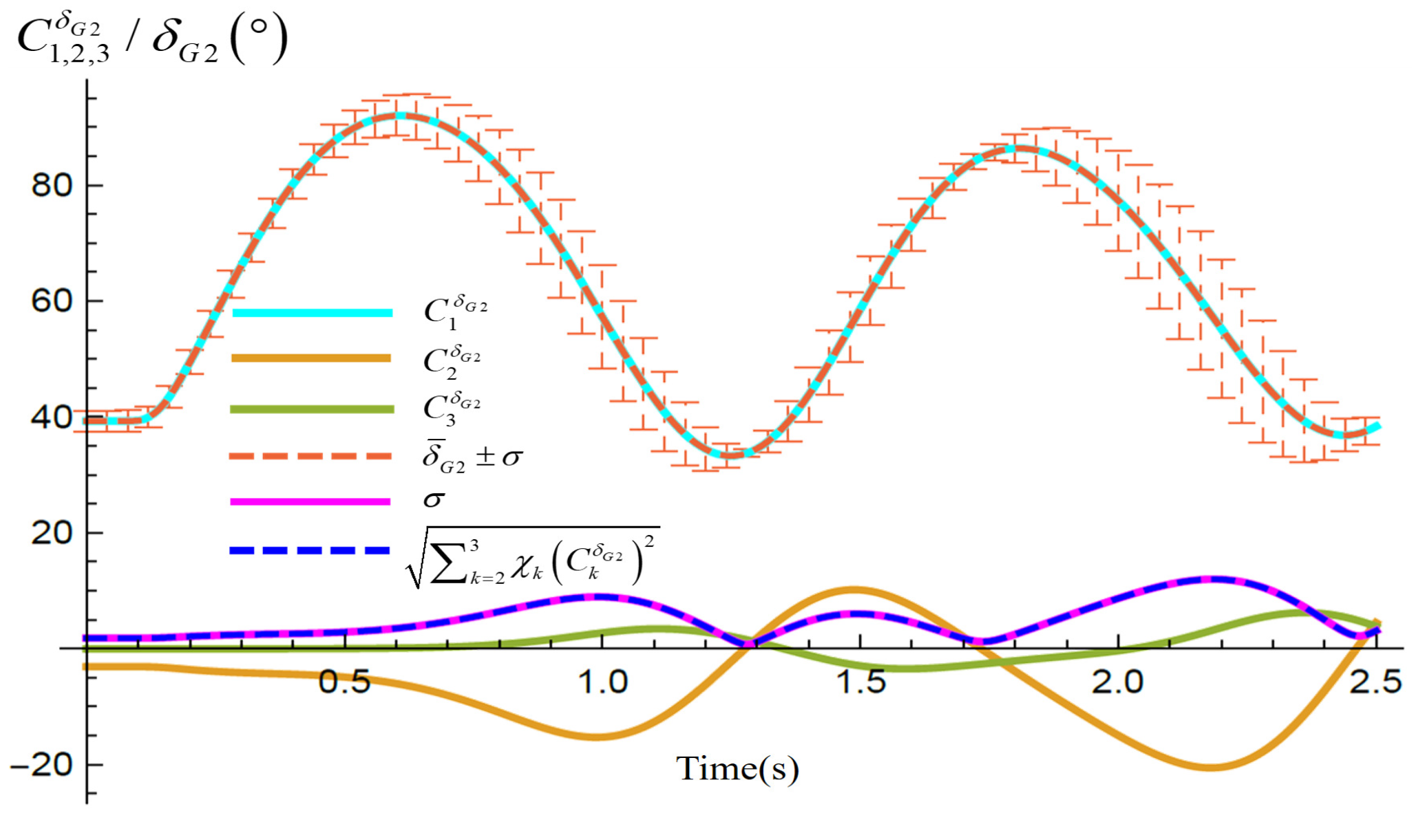
3.1. Polynomial Approximation of Transient Dynamics

As can be seen from the dynamic constraints of (5) and (6), the relationship between parameters ${\mathbf{p}}^{\prime }$ and system variables ${\mathbf{y}}^{\prime }$ is implicitly described by a set of DAEs with initial condition ${\mathbf{y}}_0^{\prime }$. To eliminate this set of DAEs from the optimization model to make the optimization model easy to solve, the SCM is introduced to approximate the relationship between ${\mathbf{y}}^{\prime }\left(t\right)$ and ${\mathbf{p}}^{\prime }$ explicitly with polynomial expression.

Because $\left|\partial \mathbf{g}/\partial \mathbf{y}\right|\ne \mathbf{0}$ for $t\in \left(t_0,t_{\mathrm{end}}\right]$ in general, according to the implicit function theorem, the relationship between ${\mathbf{y}}^{\prime }$ and ${\mathbf{p}}^{\prime }$ can be approximated by

$${\mathbf{y}}^{\prime }(t,{\mathbf{p}}^{\prime })\approx {\widehat{\mathbf{y}}}^{\prime }(t,{\mathbf{p}}^{\prime })=\sum _{k=1}^{N_{\mathrm{b}}}{\mathbf{c}}_k^{{\mathbf{y}}^{\prime }}\left(t\right){\Phi }_k\left({\mathbf{p}}^{\prime }\right),$$

(10)

where ${\Phi }_k\left({\mathbf{p}}^{\prime }\right)\triangleq \left\{{\phi }_{k_1}\left(p_1^{\prime }\right){\phi }_{k_2}\left(p_2^{\prime }\right)\cdots {\phi }_{k_i}\left(p_i^{\prime }\right)\cdots {\phi }_{k_d}\left(p_d^{\prime }\right)\right\}$ is the k-th orthogonal polynomial basis function. As N is the total degree of $\left\{\Phi \left({\mathbf{p}}^{\prime }\right)\right\}$, then $N_{\mathrm{b}}={\displaystyle \frac{(N+d)!}{N!d!}}$. In this paper, the Legendre polynomial series are selected as basis functions; thus the range of ${\mathbf{p}}^{\prime }$ is transformed to $[-1,1]$ by linear transformations.

Then, the undetermined coefficients ${\mathbf{c}}_k^{{\mathbf{y}}^{\prime }}\left(t\right)$ in (10) can be solved by the SCM with the following formula:

$${\mathbf{c}}_k^{{\mathbf{y}}^{\prime }}\left(t\right)=\frac{1}{{\chi }_k}\sum _{m=1}^M{\alpha }_m{\Phi }_k\left({\mathbf{p}}^{\prime \left(m\right)}\right){\varphi }_{{\mathbf{y}}^{\prime }}({\mathbf{y}}_0^{\prime },t,{\mathbf{p}}^{\prime \left(m\right)}),$$

(11)

where ${\chi }_k={\int }_{D^{\prime }}{\Phi }_k\left({\mathbf{p}}^{\prime }\right){\Phi }_k\left({\mathbf{p}}^{\prime }\right)\omega \left({\mathbf{p}}^{\prime }\right)\mathrm{d}{\mathbf{p}}^{\prime }$ with $\omega \left({\mathbf{p}}^{\prime }\right)=1$ for Legendre polynomial series; ${\mathbf{p}}^{\prime \left(m\right)},m=1,\dots ,M$ are collocation points (also called integration points). The collocation points and corresponding integration coefficient ${\alpha }_m$ are determined through the Smolyak sparse grid quadrature [28]; ${\varphi }_{{\mathbf{y}}^{\prime }}({\mathbf{y}}_0^{\prime },t,{\mathbf{p}}^{\prime \left(m\right)})$ is the trajectory of ${\mathbf{y}}^{\prime }$ with fault information, initial condition ${\mathbf{y}}^{\prime }\left(t_0\right)={\mathbf{y}}_0^{\prime }$ and ${\mathbf{p}}^{\prime }={\mathbf{p}}^{\prime \left(m\right)}$, which can be obtained through simulation by numerical methods. Therefore, the nonlinearity of the initial condition and the accuracy of numerical simulation results will affect the accuracy of the polynomial approximation. The common numerical integration includes Euler’s method, improved Euler’s method, implicit trapezoidal method, and Runge–Kutta method. Considering that the implicit trapezoidal method has better accuracy and numerical stability, in this paper, the implicit trapezoidal method is utilized. It can be observed in Equation (11) that ${\mathbf{c}}_k^{{\mathbf{y}}^{\prime }}\left(t\right)$ is determined by initial condition ${\mathbf{y}}_0^{\prime }$ when ${\chi }_k$, ${\alpha }_m$, ${\mathbf{p}}^{\prime \left(m\right)}$ are predesigned in SCM.

Note that polynomial approximation Equation (10) cannot reflect the statistical information of uncertain parameters. However, when their probability distribution is known, Equation (10) can be used to retrieve the statistical information of ${\mathbf{y}}^{\prime }$. For instance, if the uncertain parameters are uniformly distributed, according to the orthogonality of Legendre polynomials, the mean and standard variance of ${\mathbf{y}}^{\prime }(t,{\mathbf{p}}^{\prime })$ can be approximated as [29]

$$\begin{array}{c}\hfill {\mu }_{{\mathbf{y}}^{\prime }}\left(t\right)=\mathbb{E}\left[{\mathbf{y}}^{\prime }(t,{\mathbf{p}}^{\prime })\right]\\ \hfill \approx \int \left(\sum _{k=1}^{N_{\mathrm{b}}}{\mathbf{c}}_k^{{\mathbf{y}}^{\prime }}\left(t\right){\Phi }_k\left({\mathbf{p}}^{\prime }\right)\right)\mathrm{d}F\left({\mathbf{p}}^{\prime }\right)={\mathbf{c}}_1^{{\mathbf{y}}^{\prime }}\left(t\right),\end{array}$$

(12)

$$\begin{array}{c}\hfill {\sigma }_{{\mathbf{y}}^{\prime }}=\sqrt{\mathbb{E}\left[{({\mathbf{y}}^{\prime }(t,{\mathbf{p}}^{\prime })-{\mu }_{{\mathbf{y}}^{\prime }}\left(t\right))}^2\right]}\approx \sqrt{{\sum }_{k=2}^{N_{\mathrm{b}}}\left[{\chi }_k{\left({\mathbf{c}}_k^{{\mathbf{y}}^{\prime }}\left(t\right)\right)}^2\right]}.\end{array}$$

(13)

Figure 1 is plotted to illustrate Equations (12) and (13). The fault condition of Figure 1 is presented in Section 6.1, and the uncertain parameter $p_{\mathrm{L}5}$ is uniformly distributed in $p_{\mathrm{L}5}\in [112.5,137.5]$ MW. By setting the total degree of polynomial bases to 2, the polynomial approximation of ${\delta }_{\mathrm{G}2}$ in terms of $p_{\mathrm{L}5}$ is

$$\begin{array}{c}\hfill {\delta }_{\mathrm{G}2}\approx {\widehat{\delta }}_{\mathrm{G}2}=\sum _{k=1}^3{\mathbf{c}}_k^{\delta }\left(t\right){\Phi }_k\left(p_{\mathrm{L}5}\right).\end{array}$$

(14)

Coefficients ${\mathbf{c}}_k^{\delta }\left(t\right),k=1,2,3$ in (14) are plotted in Figure 1. As can be seen, the trajectories of ${\mathbf{c}}_1^{{\mathbf{y}}^{\prime }}\left(t\right)$ and $\sqrt{{\sum }_{k=2}^3{\chi }_k{\left({\mathbf{c}}_k^{{\delta }_{\mathrm{G}2}}\left(t\right)\right)}^2}$ are coincident with the mean trajectory ${\overline{\delta }}_{\mathrm{G}2}$ and standard variance trajectory $\sigma$ respectively, which validates Equations (12) and (13).

If uncertain parameters are not uniformly distributed, statistical quantities of ${\mathbf{y}}^{\prime }(t,{\mathbf{p}}^{\prime })$ can also be readily approximated by combining the polynomial approximation Equation (10) with sampling methods such as the Monte Carlo method and Latin hypercube sampling [24]. Note that the computation of polynomial approximation does not require the uncertain parameters to be non-independent. However, when the obtained polynomial approximation is further used to analyze the statistical properties of system variables, it is necessary to consider the correlation of the uncertain parameters.

3.2. Reformulatin of Transient Stability Constraints

After the polynomial approximation of ${\mathbf{y}}^{\prime }$ has been obtained, the polynomial expression can be used to substitute variables ${\mathbf{y}}^{\prime }$ in transient stability constraints (7). Then transient stability constraints are discreted into a series of algebraic equations with numerical discretization, such that:

$${\mathbf{H}}_{\mathrm{t}}(\sum _{k=1}^{N_b}{\mathbf{c}}_k^{{\mathbf{p}}^{\prime }}\left(t\right){\Phi }_k\left({\mathbf{y}}^{\prime }\right),{\mathbf{p}}^{\prime })\le \mathbf{0},$$

(15)

where ${\mathbf{H}}_{\mathrm{t}}={[H_{t_1},H_{t_2},\dots ,H_{t_s}]}^{\mathrm{T}}$ and s is the number of total integration steps. According to (11) and (15) can be simplified as:

$${\mathbf{H}}_{\mathrm{t}}({\mathbf{y}}_0^{\prime },{\mathbf{p}}^{\prime })\le \mathbf{0}.$$

(16)

Because all transient variables in transient stability constraints (7) have been substituted by polynomial expressions as shown in (10), the dynamic constraints (5) and (6), which define the transient outputs, are implicitly included in the reformulated transient stability constraints (16). Therefore, dynamic constraints (5) and (6) and the corresponding transient variable ${\mathbf{y}}^{\prime }$ can be eliminated from the model of Pa-TSCOPF, and the following algebraic Pa-NLP which eliminates differential equations is formulated:

$$\underset{{\mathbf{y}}_0^{\prime },\mathbf{u}}{min}c({\mathbf{y}}_0^{\prime },\mathbf{u},\mathbf{p})$$

(17)

subject to:

$$\mathbf{0}=\mathbf{G}({\mathbf{y}}_0^{\prime },\mathbf{u},\mathbf{p})$$

(18)

$${\mathbf{H}}_{0.\mathrm{mim}}\le {\mathbf{H}}_0({\mathbf{y}}_0^{\prime },\mathbf{u},\mathbf{p})\le {\mathbf{H}}_{0.\max }$$

(19)

$${\mathbf{H}}_{\mathrm{t}}({\mathbf{y}}_0^{\prime },\mathbf{u},\mathbf{p})\le \mathbf{0}.$$

(20)

The elimination of the dynamic constraints (5) and (6) from the parametric TSCOPF model gives the following advantages:

(1)

The effect of uncertain parameters $\mathbf{p}$ on the transient process can be explicitly evaluated by the transient stability constraint (20), which is a series of polynomials and easy to be evaluated in the Pa-TSCOPF problem.

(2)

The dynamic constraints (5) and (6) in the general Pa-TSCOPF model is a set of DAEs, which cannot be dealt with directly by existing optimization methods. Differently, the solution for the algebraic Pa-NLP in the reformulated Pa-TSCOPF model is easier to be dealt with.

4. Solution of Algebraic Pa-NLP Model Based on the Stochastic Collocation Method

The existence of uncertain parameters $\mathbf{p}$ in the proposed algebraic Pa-NLP model implies the optimal steady state operating point ${\mathbf{y}}_0^{\prime *}\left(\mathbf{p}\right)$ and the optimal control scheme ${\mathbf{u}}^{*}\left(\mathbf{p}\right)$ depend on uncertain parameters $\mathbf{p}$. The challenge for solving the algebraic Pa-NLP is how to effectively evaluate the effect of uncertain parameters $\mathbf{p}$ on the optimal solution. The SCM-based optimization method proposed here is a parametric optimization method for algebraic Pa-NLP. It aims to approximate the relationship between the Pa-TSCOPF solution and uncertain parameters explicitly by polynomial expressions. This method starts with the formulation of parametric Karush–Kuhn–Tucker (KKT) conditions by the primal–dual interior point method (PDIPM) and gets the parametric optimal solution by applying the SCM to solve KKT conditions.

4.1. Parametric KKT Conditions of Algebraic Pa-NLP Model

Based on the classical PDIPM [40], by introducing slack variables for inequality constraints (19) and (20) and appending the logarithmic barrier functions to the objective, algebraic Pa-NLP model (17)–(20) can be reformulated as the following subproblem:

$$\begin{array}{c}\hfill \underset{{\mathbf{y}}_0^{\prime },\mathbf{u}}{min}c({\mathbf{y}}_0^{\prime },\mathbf{u},\mathbf{p})-\mathbf{\mu }\sum _{j=1}^{r_0}log\left(\mathbf{l}\left(\mathbf{p}\right)\right)-\mathbf{\mu }\sum _{j=1}^{r_0}log\left(\mathbf{\upsilon }\left(\mathbf{p}\right)\right)\\ \hfill -\mathbf{\mu }\sum _{j=1}^{r_{\mathrm{t}}}log\left({\mathbf{\upsilon }}_{\mathrm{t}}\left(\mathbf{p}\right)\right)\end{array}$$

(21)

subject to:

$$\mathbf{0}=\mathbf{G}({\mathbf{y}}_0^{\prime },\mathbf{u},\mathbf{p})$$

(22)

$${\mathbf{H}}_0({\mathbf{y}}_0^{\prime },\mathbf{u},\mathbf{p})+\mathbf{\upsilon }\left(\mathbf{p}\right)={\mathbf{H}}_{0.\max }$$

(23)

$${\mathbf{H}}_0({\mathbf{y}}_0^{\prime },\mathbf{u},\mathbf{p})-\mathbf{l}\left(\mathbf{p}\right)={\mathbf{H}}_{0.\min }$$

(24)

$${\mathbf{H}}_{\mathrm{t}}({\mathbf{y}}_0^{\prime },\mathbf{u},\mathbf{p})+{\mathbf{\upsilon }}_{\mathrm{t}}\left(\mathbf{p}\right)=\mathbf{0},$$

(25)

where $\mathbf{l}=[l_1\left(\mathbf{p}\right),\dots ,l_r\left(\mathbf{p}\right)]$, $\mathbf{\upsilon }=[{\upsilon }_1\left(\mathbf{p}\right),\dots ,{\upsilon }_r\left(\mathbf{p}\right)]$, ${\mathbf{\upsilon }}_{\mathrm{t}}=[{\upsilon }_{\mathrm{t}1}\left(\mathbf{p}\right),\dots ,{\upsilon }_{\mathrm{t}s}\left(\mathbf{p}\right)]$ are the slack variables for inequality constraints respectively, and r, s are the numbers of steady-state inequality constraints (19) and transient stability inequality constraints (20). As $\mathbf{\mu }$ tends towards zero, the solution of the reformulated subproblem approaches the solution of the primary optimization model (17)–(20).

The Lagrange function of the subproblem (21)–(25) is

$$\begin{array}{c}\hfill {\mathbf{L}}_{\mu }=c(\overline{\mathbf{y}},\mathbf{p})-{\xi }^{\mathrm{T}}\left(\mathbf{p}\right)\mathbf{G}(\overline{\mathbf{y}},\mathbf{p})\\ \hfill -{\mathbf{z}}^{\mathrm{T}}\left(\mathbf{p}\right)[{\mathbf{H}}_0(\overline{\mathbf{y}},\mathbf{p})+\mathbf{\upsilon }\left(\mathbf{p}\right)-{\mathbf{H}}_{0.\max }]\\ \hfill -{\mathbf{w}}^{\mathrm{T}}\left(\mathbf{p}\right)[{\mathbf{H}}_0(\overline{\mathbf{y}},\mathbf{p})+\mathbf{l}\left(\mathbf{p}\right)-{\mathbf{H}}_{0.\min }]\\ \hfill -{\mathbf{\gamma }}^{\mathrm{T}}\left(\mathbf{p}\right)[{\mathbf{H}}_{\mathrm{t}}(\overline{\mathbf{y}},\mathbf{p})+{\mathbf{\upsilon }}_{\mathrm{t}}\left(\mathbf{p}\right)]\\ \hfill -\mathbf{\mu }\sum _{j=1}^{r_0}log\left(\mathbf{l}\left(\mathbf{p}\right)\right)-\mathbf{\mu }\sum _{j=1}^{r_0}log\left(\mathbf{\upsilon }\left(\mathbf{p}\right)\right)\\ \hfill -\mathbf{\mu }\sum _{j=1}^{r_{\mathrm{t}}}log\left({\mathbf{\upsilon }}_{\mathrm{t}}\left(\mathbf{p}\right)\right),\end{array}$$

(26)

where $\mathbf{\xi }\left(\mathbf{p}\right)$, $\mathbf{z}\left(\mathbf{p}\right)$, $\mathbf{w}\left(\mathbf{p}\right)$, $\mathbf{\gamma }\left(\mathbf{p}\right)$ are Lagrange multipliers (dual variables) for constraints (22)–(25) respectively. The optimal solution of the subproblem (21)–(25) satisfies KKT first-order conditions:

$$\begin{array}{c}\hfill {\nabla }_{{\mathbf{y}}_0^{\prime }}{\mathbf{L}}_{\mu }\equiv {\nabla }_{{\mathbf{y}}_0^{\prime }}\mathbf{c}(\overline{\mathbf{y}},\mathbf{p})-{\nabla }_{{\mathbf{y}}_0^{\prime }}\mathbf{G}(\overline{\mathbf{y}},\mathbf{p})\mathbf{\xi }\\ \hfill -{\nabla }_{{\mathbf{y}}_0^{\prime }}{\mathbf{H}}_0(\overline{\mathbf{y}},\mathbf{p})(\mathbf{w}+\mathbf{z})-{\nabla }_{{\mathbf{y}}_0^{\prime }}{\mathbf{H}}_{\mathrm{t}}(\overline{\mathbf{y}},\mathbf{p})\mathbf{\gamma }=0\end{array}$$

(27)

$${\nabla }_{\mathbf{\xi }}{\mathbf{L}}_{\mu }\equiv \mathbf{G}(\overline{\mathbf{y}},\mathbf{p})=0$$

(28)

$${\nabla }_{\mathbf{z}}{\mathbf{L}}_{\mu }\equiv {\mathbf{H}}_0(\overline{\mathbf{y}},\mathbf{p})-\mathbf{l}\left(\mathbf{p}\right)-{\mathbf{H}}_{0.\min }=0$$

(29)

$${\nabla }_{\mathbf{w}}{\mathbf{L}}_{\mu }\equiv {\mathbf{H}}_0(\overline{\mathbf{y}},\mathbf{p})-\mathbf{\upsilon }\left(\mathbf{p}\right)-{\mathbf{H}}_{0.\max }=0$$

(30)

$${\nabla }_{\mathbf{\gamma }}{\mathbf{L}}_{\mu }\equiv {\mathbf{H}}_{\mathrm{t}}(\overline{\mathbf{y}},\mathbf{p})+{\mathbf{\upsilon }}_{\mathrm{t}}\left(\mathbf{p}\right)=0$$

(31)

$${\nabla }_{\mathbf{l}}{\mathbf{L}}_{\mu }\equiv \mathbf{L}\mathbf{Z}\mathbf{e}-\mathbf{\mu }\mathbf{e}=0$$

(32)

$${\nabla }_{\mathbf{\upsilon }}{\mathbf{L}}_{\mu }\equiv \mathbf{U}\mathbf{W}\mathbf{e}+\mathbf{\mu }\mathbf{e}=0$$

(33)

$${\nabla }_{{\mathbf{\upsilon }}_{\mathrm{t}}}{\mathbf{L}}_{\mu }\equiv {\mathbf{U}}_{\mathrm{t}}\mathbf{R}\mathbf{e}=0,$$

(34)

where $\mathbf{e}={[1,\dots ,1]}^{\mathrm{T}}$, $\mathbf{L}=\mathrm{diag}(l_1,\dots ,l_r)$, $\mathbf{Z}=\mathrm{diag}(z_1,\dots ,z_r)$, $\mathbf{U}=\mathrm{diag}({\upsilon }_1,\dots ,{\upsilon }_r)$, $\mathbf{W}=\mathrm{diag}(w_1,\dots ,w_r)$, ${\mathbf{U}}_{\mathrm{t}}=\mathrm{diag}({\upsilon }_{\mathrm{t}1},\dots ,{\upsilon }_{\mathrm{t}s})$, $\mathbf{R}=\mathrm{diag}({\gamma }_1,\dots ,{\gamma }_s)$.

So far, the algebraic Pa-NLP model (17)–(20) is translated into a group of parametric KKT conditions (27)–(34). We will use the SCM introduced in Section 3.2 to find the polynomial approximations of the implicit functions mapping parameters $\mathbf{p}$ to the optimal solution.

4.2. Parametric Solution of Parametric TSCOPF Model

In Section 3.2, the way to apply the SCM to reformulate DAEs as algebraic equations has been presented; therefore, to avoid redundancy, here we will only pay attention to how to solve the parametric KKT conditions (27)–(34) using the SCM.

First, all variables in KKT conditions (27)–(34) can be represented as linear combinations of the polynomial basis functions $\left\{\Phi \left(\mathbf{p}\right)\right\}$ as follows:

$$\mathbf{\varpi }\left(\mathbf{p}\right)\approx \widehat{\overline{\mathbf{\varpi }}}\left(\mathbf{p}\right)=\sum _{k=1}^{N_{\mathrm{b}}}{\mathbf{c}}_k^{\varpi }{\Phi }_k\left(\mathbf{p}\right),$$

(35)

where $\mathbf{\varpi }=[{\overline{\mathbf{y}}}^{\mathrm{T}},{\mathbf{\xi }}^{\mathrm{T}},{\mathbf{l}}^{\mathrm{T}},{\mathbf{\upsilon }}^{\mathrm{T}},{\mathbf{\upsilon }}_{\mathrm{t}}^{\mathrm{T}},{\mathbf{z}}^{\mathrm{T}},{\mathbf{w}}^{\mathrm{T}},{\mathbf{\gamma }}^{\mathrm{T}}]$ is the compact form of variables in KKT conditions.

Then, by the SCM introduced in Section 3.2 the unknown coefficients ${\mathbf{c}}_k^{\varpi }$ can be solved:

$${\mathbf{c}}_k^{\varpi }\left(t\right)=\frac{1}{{\chi }_k}\sum _{m=1}^M{\alpha }_m{\Phi }_k\left({\mathbf{p}}^{\left(m\right)}\right)\varpi \left({\mathbf{p}}^{\left(m\right)}\right),$$

(36)

where $\varpi \left({\mathbf{p}}^{\left(m\right)}\right)$ is the solution of parametric KKT conditions (27)–(34) with $\mathbf{p}={\mathbf{p}}^{\left(m\right)}$.

So far, the parametric optimal solution (35) of the initial parametric TSCOPF (1)–(7) has been obtained by the SCM. The parameterized optimal solution contains polynomial approximation for the optimal control parameters, system states, slack variables, and Lagrange multipliers, which explicitly describes the quantitative relationship between the Pa-TSCOPF solution and uncertain parameters.

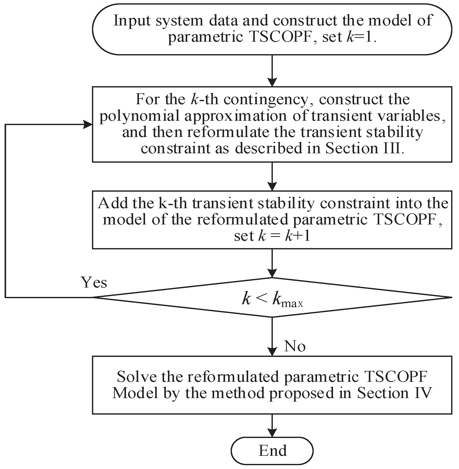
5. Procedures of Parametric TSCOPF in Multi-Contingency Case

The preceding sections have introduced how to use the SCM to solve the Pa-TSCOPF considering a single contingency. In practical applications, when multiple contingencies are considered, the corresponding transient stability constraints need to be reformulated separately for each contingency according to the proposed method. The main procedures of the proposed method for solving the parametric TSCOPF problem in multi-contingency case are summarized below and depicted in Figure 2.

Step 1:

Input system data and construct the parametric TSCOPF model. Determine the $k_{\max }$ contingencies to be considered in the transient stability analysis and set $k=1$.

Step 2:

For the k-th contingency, construct the polynomial approximation of transient variables as (10), and then the k-th transient stability constraint in parametric TSCOPF model can be reformulted as (20).

Step 3:

Add the k-th trainsient stability constraint into the reformulated model of the parametric TSCOPF, set $k=k+1$.

Step 4:

If $k<k_{\max }$, return to step 2. If $k=k_{\max }$, solve the reformulated model of parametric TSCOPF (17)–(20) by the method proposed in Section 4; the polynomial formulation (35) with coefficient solved by (36) is the parametric optimal solution of the reformulated parametric TSCOPF problem.

6. Case Studies

The 3-machine, 9-bus system case is used to verify the theoretical validity of the proposed method. In addition, because it is difficult to obtain the transient parameters of an actual power system, we use the IEEE 145-bus system to verify the feasibility of the proposed method in practical power systems. All computations are performed on Wolfram Mathematica 12.0 on a laptop with a CPU of Intel i5-6200U 2.30 GHz and a RAM of 4.0 GB, and the time step of numerical integration is $0.01\mathrm{s}$.

6.1. 3-Machine 9-Bus System Case

6.1.1. Case Settings

The detailed data of the 3-machine, 9-bus system shown in Figure 3 can be found in [31]. The mechanical power of generators is assumed to remain constant during the transient process, and the dynamic models for transient stability analysis are 4th order models equipped with IEEE Type 1 exciter which is cited from [16]. The slack generator is at bus 1. The controllable parameters are power generation $P_{\mathrm{G}2}\in [130,155]$ MW and $P_{\mathrm{G}3}\in [45,155]$ MW.

Two fault scenarios are considered in this case study: fault 1 involves a three-phase fault on line $5–7$ at the bus 7 end at $t=0.1\mathrm{s}$, which is cleared after $t_{\mathrm{cl}}=0.07\mathrm{s}$ by tripping the faulted line $5–7$; fault 2 is a three-phase fault on line $4–5$ at the bus 4 end at $t=0.1\mathrm{s}$, which is cleared after $t_{\mathrm{cl}}=0.2\mathrm{s}$ by tripping this faulted line.

There are 3 uncertain parameters allowed to vary, i.e., the real power $P_{\mathrm{L}5}$, $P_{\mathrm{L}6}$, $P_{\mathrm{L}8}$ of the load at bus 5, bus 6, and bus 8, whose variation ranges are $P_{\mathrm{L}5}\in [112.5,137.5]\mathrm{MW}$, $P_{\mathrm{L}6}\in [81,99]\mathrm{MW}$, $P_{\mathrm{L}8}\in [90,110]\mathrm{MW}$.

The objective function is defined as the traditional operating cost:

$$C_{\mathrm{G}}=\sum _{i=1}^3(a_i{P}_{\mathrm{G}i}^2+b_i{P}_{\mathrm{G}i}+c_i),$$

(37)

where $P_{\mathrm{G}i}$ is active power of the i-th generator. ${[a_1,a_2,a_3]}^{\mathrm{T}}={[2,1,1]}^{\mathrm{T}}$, ${[b_1,b_2,b_3]}^{\mathrm{T}}={[3,1,1]}^{\mathrm{T}}$ and ${[c_1,c_2,c_3]}^{\mathrm{T}}={[3,1,1]}^{\mathrm{T}}$ are the fuel cost coefficients of generators.

The steady state constraint is that voltages of PQ buses are required to be in range $[0.95,1.05]$ p.u. The transient stability constraint is defined as the following inequality constraints:

$${\delta }_{\mathrm{G}i}={\delta }_{\mathrm{G}}^i-\frac{{\sum }_{k=1}^{N_{\mathrm{G}}}{H}_k{\delta }_{\mathrm{G}}^k}{{\sum }_{k=1}^{N_{\mathrm{G}}}{H}_k}\le {\delta }_{\mathrm{G}i.\max },t\in (t_0,t_{\mathrm{end}}],$$

(38)

where $H_k$ is inertia constant of the k-th generator, ${\delta }_{\mathrm{G}}^i$ is the rotor angle of the i-th generator and ${\delta }_{\mathrm{G}i}$ is its relative rotor angle with respect to the center of inertia reference frame. ${\delta }_{\mathrm{G}i.\max }$ is the upper limit of the rotor angle. It should be noted that other constraints, such as voltage dips or rises and line flow limits can also be included in transient stability constraints.

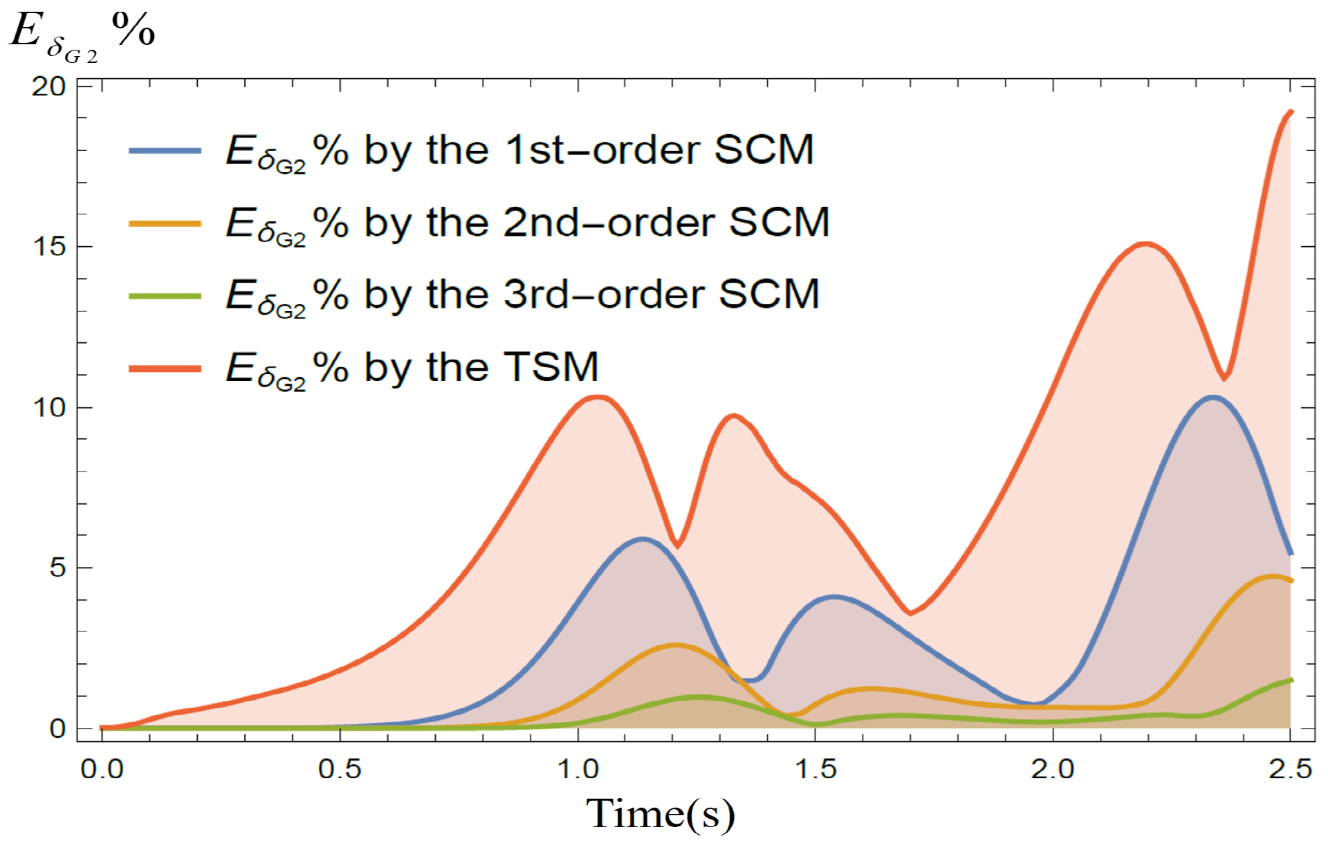
6.1.2. Approximation Error and Computation Time

To show the accuracy of the proposed method for the approximation of transient variables, fault 1 is taken as an example and the trajectory of ${\delta }_{\mathrm{G}2}$ is plotted in Figure 4 to compare the approximation error of the proposed stochastic collocation method (SCM) and the trajectory sensitivity method (TSM), where the results of the numerical simulation method are used as a benchmark. The nominal trajectory of ${\delta }_{\mathrm{G}2}$, shown as a black line in Figure 4, is obtained with the parameter variation $△P_{\mathrm{L}}={[△P_{\mathrm{L}5},△P_{\mathrm{L}6},△P_{\mathrm{L}8}]}^{\mathrm{T}}=0$ by the numerical simulation method (NSM). Approximated trajectories were then formed for $△P_{\mathrm{L}}=\pm 7.5\%P_{\mathrm{L}0}$, where $P_{\mathrm{L}0}$ is the expected value of $P_{\mathrm{L}}$. These approximated trajectories are shown as dashed lines for the SCM with $N=2$ and dotted lines for the TSM respectively. For comparison, corresponding exact (fully simulated) trajectories are shown as solid lines. As we can see, the approximations obtained by the proposed SCM presented in this example are very accurate with parameter variation $\pm 7.5\%P_{\mathrm{L}}$. Both the proposed method and the trajectory sensitivity-based approximation tracked the exact trajectory quite closely before $t=0.5\mathrm{s}$. After that time, the approximation error of the trajectory sensitivities increased obviously. To quantitatively evaluate the approximation error, we use the mean absolute percentage error (MAPE) $E_{{\mathrm{y}}^{\prime }}\%$ as the error index:

$$E_{{\mathrm{y}}^{\prime }}\%\left(t\right)\triangleq \frac{100}{n}\sum _{i=1}^n\left|\frac{y^{\prime }\left(t\right)-\widehat{y^{\prime }}\left(t\right)}{y^{\prime }\left(t\right)}\right|,$$

(39)

where n is the number of simulation points.

Figure 5 plots the MAPE of rotor angle $E_{{\delta }_{\mathrm{G}2}}\%$ versus time t, and

Table 1. Computation time and approxiamtion error of the SCM and TSM in fault 1.

Method	${\overline{\mathit{E}}}_{{\mathit{\delta }}_{\mathit{G}1}}\%$1	${\overline{\mathit{E}}}_{{\mathit{\delta }}_{\mathit{G}2}}\%$1	${\overline{\mathit{E}}}_{{\mathit{\delta }}_{\mathit{G}3}}\%$1	${\mathit{N}}_{\mathbf{p}}$2	Total Time
TSM	$38.29\%$	$6.91\%$	$13.11\%$	-	8.548 s
SCM, $N=1$	$2.45\%$	$2.78\%$	$1.84\%$	7	12.125 s
SCM, $N=2$	$0.88\%$	$0.98\%$	$0.73\%$	25	45.75 s
SCM, $N=3$	$0.27\%$	$0.30\%$	$0.24\%$	69	136.766 s

¹${\overline{E}}_{{\delta }_{G1}}\%$, ${\overline{E}}_{{\delta }_{G2}}\%$, ${\overline{E}}_{{\delta }_{G3}}\%$ are mean values of $E_{{\delta }_{G1}}\%$, $E_{{\delta }_{G2}}\%$, $E_{{\delta }_{G3}}\%$. ² $N_{\mathrm{p}}$ is the number collocation points of the SCM.

shows the average MAPE ${\overline{E}}_{{\delta }_{\mathrm{G}}}\%$ and computation time of the TSM and the SCM with different order N. It can be seen from Figure 5 that, no matter what N is, $E_{{\delta }_{\mathrm{G}2}}\%$ with the SCM during the whole time domain is smaller than that of the TSM. However, from Table 1 we can see that though the SCM’s average RMSE is much smaller than that of TSM, it needs more computation time in the respect that it requires a small number of simulations at the collocation points. Moreover, for the SCM, when $N=3$, although the average MAPE is reduced compared to that of $N=2$, more computation time is required. This is because the higher N, the more collocation points are needed for the SCM, which leads to more computation time. So it is suggested that $N=2$ is sufficient for analysis of transient stability to retain both accuracy and efficiency in the general case.

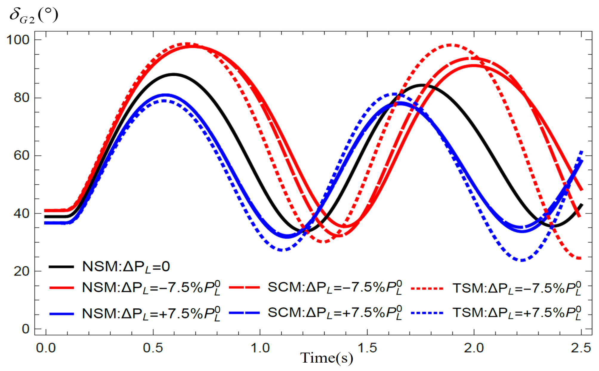
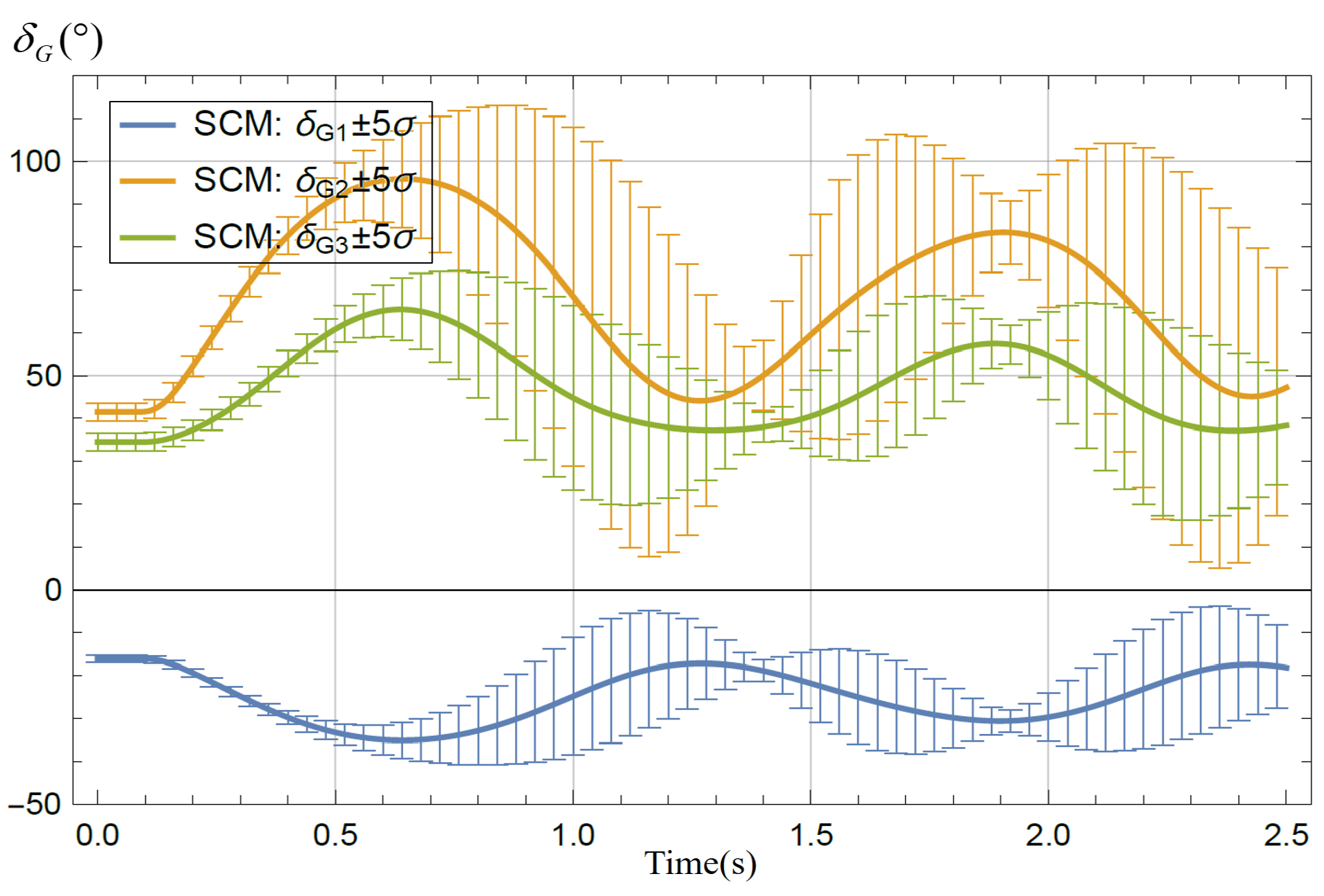
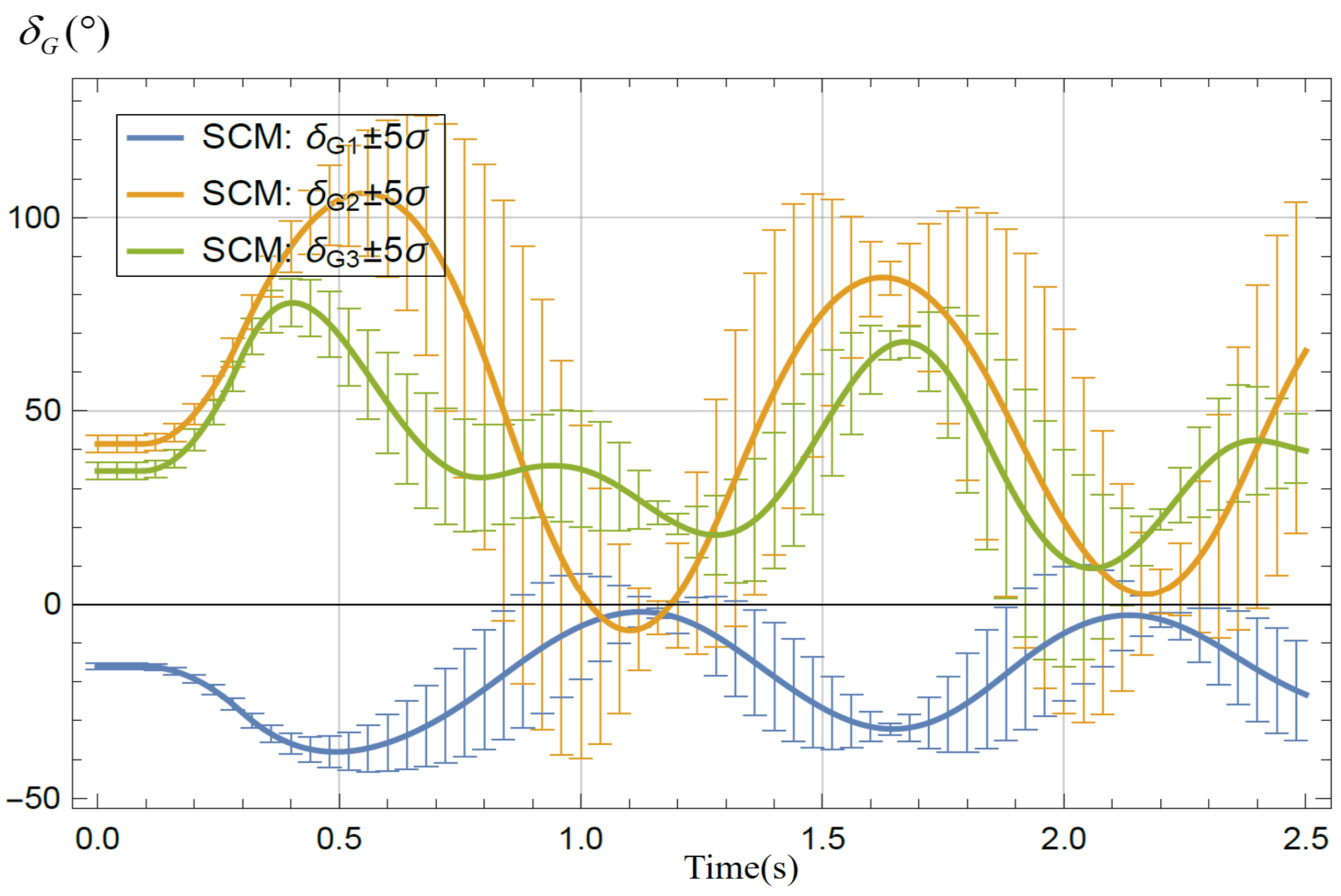
6.1.3. Transient Stability Analysis of the Initial Operation Point

Because the polynomial approximation of transient variables concerning the uncertain parameters has been formed, their expectation and standard variance can be easily obtained by using Equations (10) and (11). When no preventive control is applied in the fault 1 and fault 2, the expectation trajectories of relative rotor angles ${\delta }_{\mathrm{G}1},{\delta }_{\mathrm{G}2},{\delta }_{\mathrm{G}3}$ with respect to a center of inertia reference frame and their standard deviation are plotted in Figure 6 and Figure 7, which are obtained through Equations (12) and (13).

As we can see, the trajectories of rotor angles will be affected by uncertain parameters in both faults. According to Chebyshev’s inequality, for a variable with any distribution, at least $93.75\%$ of the data were within 4 standard deviations of the expectation, or a little more conservative, at least $96\%$ were within 5 standard deviations of the expectation. Therefore, in fault 1, the possible maximum rotor angles is ${\delta }_{\mathrm{G}2}={87.63}^{\circ }+5\times {5.08}^{\circ }={113.035}^{\circ }$ at $t=0.84\mathrm{s}$. In fault 2, the possible maximum rotor angles is ${\delta }_{\mathrm{G}2}={101.17}^{\circ }+5\times {5.0}^{\circ }={126.44}^{\circ }$ at $t=0.64\mathrm{s}$. The maximum rotor angles in the critical stable scenario are ${\delta }_{\mathrm{G}2}={114.3}^{\circ }$ in fault 1 and ${\delta }_{\mathrm{G}2}={138.73}^{\circ }$ in fault 2 respectively. Therefore, affected by uncertain parameters, the initial operation point without preventive control is close to the critical stable scenario, and hence the implementation of parametric TSCOPF is needed. For the consideration of safety, we set the upper limit of the relative swing angle as ${80}^{\circ }$ for fault 1 and ${100}^{\circ }$ for fault 2 in (38).

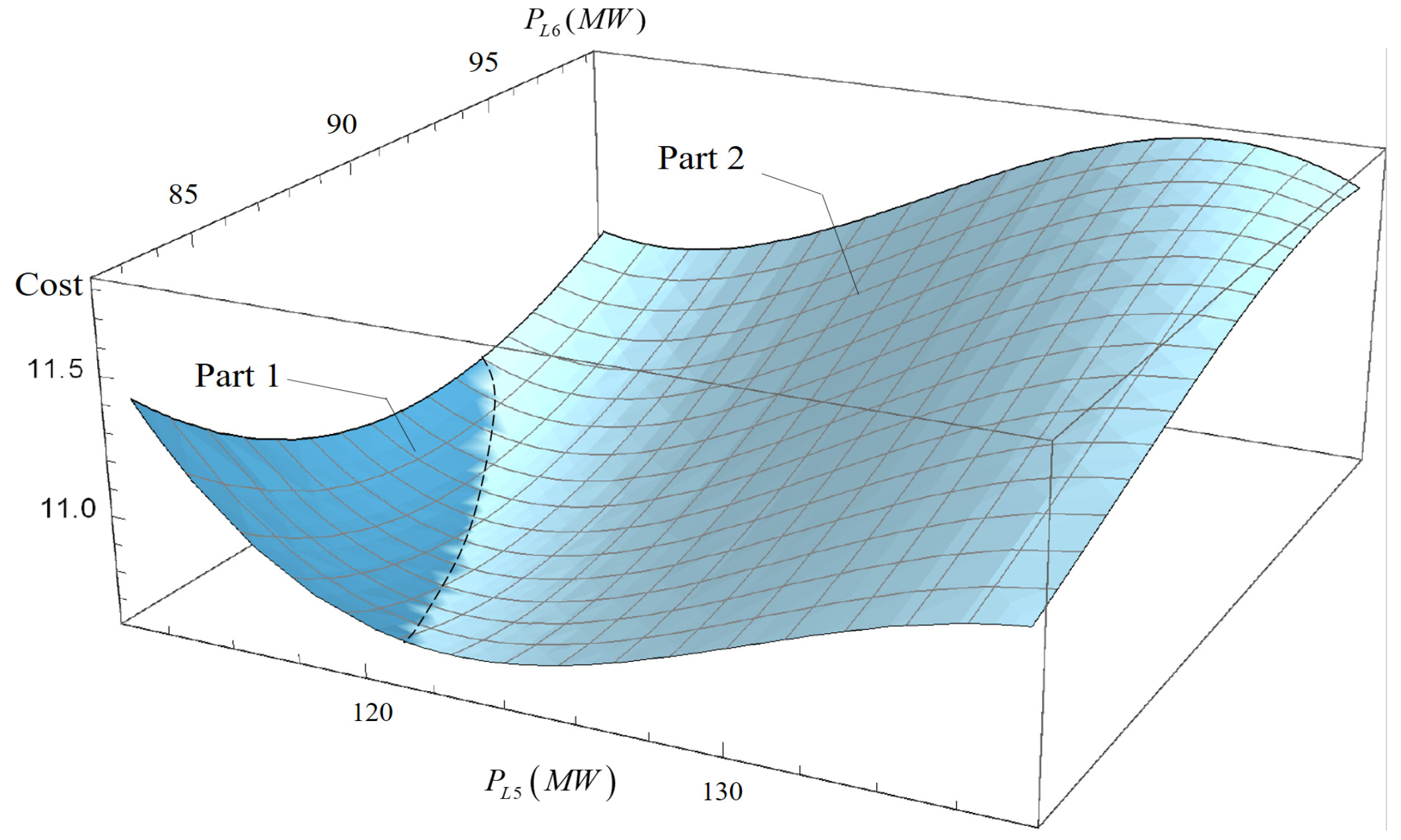
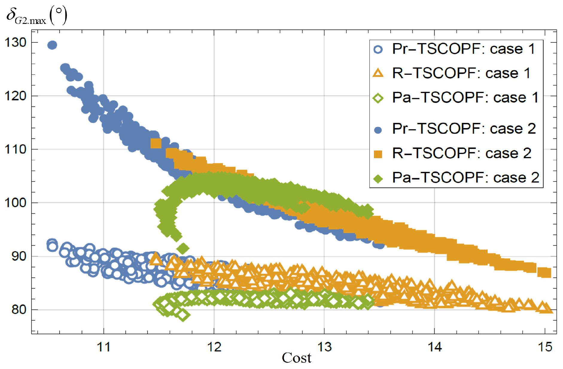
6.1.4. Solution of the Parametric TSCOPF Problem

To show how the optimal solution varies with uncertain parameters, we make $P_{\mathrm{L}8}$ be fixed to $100\mathrm{MW}$, and hence objective function becomes a function of $P_{\mathrm{L}5}$ and $P_{\mathrm{L}6}$, which forms a surface as shown in Figure 8. As we can see, the surface obtained by the proposed method is composed of 2 parts, part 1 in dark blue is transient stability constrained as ${\delta }_{\mathrm{G}2}$ encountering its upper limit in fault 2, whereas part 2 in light blue is transient stability constrained as ${\delta }_{\mathrm{G}2}$ encountering its upper limit in fault 1. When $P_{\mathrm{L}5}$ or $P_{\mathrm{L}6}$ decreases to the dashed line where part 1 and part 2 intersect, the encountering of the transient stability constraint is transformed from fault 1’s to fault 2’s. The RMSE in the whole parameter domain is 0.09 (about $0.83\%$ compared to the mean value of the objective function), showing good accuracy of the proposed approximation.

Furthermore, 500 pairs of the uncertain parameters are generated to compare the performance of the parametric control scheme obtained by the proposed Pa-TSCOPF with the control scheme obtained by the Pr-TSCOPF and R-TSCOPF. Note that for R-TSCOPF and Pa-TSCOPF with a $15\%$ probability of allowing constraints violation, ${\delta }_{\mathrm{G}2}\le {80}^{\circ }$ in fault 1 and ${\delta }_{\mathrm{G}2}\le {100}^{\circ }$ in fault 2 can not be satisfied. Therefore, the transient stability constraints are relaxed to ${\delta }_{\mathrm{G}2}\le {90}^{\circ }$ and ${\delta }_{\mathrm{G}2}\le {115}^{\circ }$ in fault 1 and fault 2 respectively.

Figure 9 plots the results in terms of the cost $C_{\mathrm{G}}$ and the maximum rotor angle ${\delta }_{\mathrm{G}2.\max }$ by different methods: (1) When the proposed Pa-TSCOPF is implemented, ${\delta }_{\mathrm{G}2.\max }$ is controlled to be lower than ${85}^{\circ }$ in fault 1 and ${105}^{\circ }$ in fault 2. (2) Assume that the uncertain parameters are uniformly distributed over their range, when the Pr-TSCOPF with $\beta =0.9.$ and R-TSCOPF are implemented, because there does not exist an optimal control scheme such that ${\delta }_{\mathrm{G}2.\max }\le {85}^{\circ }$ in fault 1 and ${\delta }_{\mathrm{G}2.\max }\le {105}^{\circ }$ in fault 2 are satisfied simultaneously, the transient constraints in Pr-TSCOPF and R-TSCOPF are relaxed to ${\delta }_{\mathrm{G}2.\max }\le {90}^{\circ }$ in fault 1 and ${\delta }_{\mathrm{G}2.\max }\le {110}^{\circ }$ in fault 2. As shown in Figure 9, it can be seen that in comparison with the Pa-TSCOPF and Pr-TSCOPF, although the cost of Pr-TSCOPF is generally lower, the transient stability constraint at many sampling points has been violated and the transient stability of the system under the influence of parameter uncertainty is not guaranteed; whiereas in comparison with the Pa-TSCOPF and R-TSCOPF, although the transient stability margin of the sampling results of R-TSCOPF is larger, the cost of the control scheme is generally higher than that of the Pa-TSCOPF.

The corresponding conclusions can also be obtained from the results in

Table 2. Comparison of optimization results of different methods in 3-machine, 9-bus system case.

Method	Mean of ${\mathit{\delta }}_{\mathit{G}2.\mathbf{max}}$		Mean of Cost	Out-of-Limit Probability
	Case1	Case2		Case1	Case2
Pr-TSCOPF	${87.51}^{\circ }$	${102.44}^{\circ }$	12.35	11.8%	10.4%
R-TSCOPF	${86.37}^{\circ }$	${97.66}^{\circ }$	13.11	2.2%	0.4%
Pa-TSCOPF	${84.00}^{\circ }$	${102.04}^{\circ }$	12.34	0.2%	0.0%

, which show that, compared with the other two methods, the control scheme provided by Pa-TSCOPF not only minimizes the out-of-limit probability of transient constraints but also makes the average cost of the control scheme relatively low. Therefore, the advantage of the proposed Pa-TSCOPF is to provide the most economical solution while maintaining the transient stability of the system. It should be noted that because the polynomial approximation still has a certain approximation error, the out-of-limit probability of transient constraints in fault 1 and fault 2 is $0.2\%$ and $0\%$, respectively. That is to say, the proposed method may not be able to guarantee $100\%$ transient stability of the system. Besides, once the parametric solution of the Pa-TSCOPF is obtained, the optimal control scheme obtained by this parametric solution is indeed essentially equal to the deterministic TSCOPF. In practice, they both obtain the solution of TSCOPF based on the measurement results of uncertain parameters, and then apply the optimal control scheme to the power system. However, the computation time required to obtain the preventive control scheme through the solution of Pa-TSCOPF (around 0.0 s in this case) is much less than the computation time required to implement a deterministic TSCOPF (2.296 s in this case). Therefore, compared with the deterministic TSCOPF, the proposed Pa-TSCOPF can provide a preventive control scheme according to the real-time operating state of the power system in a more timely manner.

6.2. IEEE 145-Bus System Case

The detailed data of the IEEE 145-bus system can be found in [41]. In this case, three wind farms are added at bus 101, bus 105, and bus 112 to verify the effectiveness of the proposed method, and each wind farm consists of 100 DFIGs with rated power 1.5 MW, whose parameters are cited from [42]. Therefore, the variation range of the uncertain wind power generation $P_{\mathrm{W}101}$, $P_{\mathrm{W}105}$, $P_{\mathrm{W}112}$ is $[0,150]$ MW.

The fault scenario considered in this case is a three-phase fault occurring at one end of line 1–6 near bus 6 at $t=0.1\mathrm{s}$, and subsequently cleared by tripping line 1–6 after a time period $t_{\mathrm{cl}}=0.12\mathrm{s}$. Considering some generators have little influence on transient stability, to avoid adverse effects on the convergence and calculation efficiency of optimization due to too many parameters, the trajectory sensitivity method is used to screen the critical generators. Therefore, the control parameters in this case are the power generation by generators at bus 89, bus 98, bus 100, and bus 104, which are assumed to vary in the range of 80∼$120\%$ of their nominal values.

By the SCM, the expectation rotor angle trajectories of several generators affected by wind speed and control parameters in the base case are plotted in Figure 10. Note that the expected trajectories and standard variance in Figure 10 are obtained by combining the polynomial approximation with the sampling-based Monte Carlo method. As we can see, the magnitude of ${\delta }_{\mathrm{G}104}$’s expectation trajectory is the highest among all generators, whose approximated possible maximum rotor angle is ${\delta }_{\mathrm{G}104}={136.152}^{\circ }+5\times {23.653}^{\circ }={254.417}^{\circ }$ at $t=1.24\mathrm{s}$. The maximum rotor angle in the critical stable scenario is ${\delta }_{\mathrm{G}104}={182.935}^{\circ }$. Therefore, affected by uncertain parameters and control parameters, the optimal operation point without considering transient stability constraints can be transiently unstable; thus the implementation of preventive control is required. The parametric TSCOPF model is the same as that of the first case. The upper limit of the relative rotor angle is set to ${135}^{\circ }$ in this case.

The parametric TSCOPF model is solved by using the proposed approach, and the results are shown in

Table 3. Parametric Control Scheme of the IEEE 145-bus system case.

Control Paramter	Parametric Control Scheme
$P_{\mathrm{G}89}$	$202.356-0.0011872P_{\mathrm{W}101}-0.0066261P_{\mathrm{W}105}$ $-0.001142P_{\mathrm{W}112}$
$P_{\mathrm{G}98}$	$35016-778.754P_{\mathrm{W}101}+124.31P_{\mathrm{W}101}^2$ $-4074.73P_{W105}+1.34181P_{\mathrm{W}101}{P}_{\mathrm{G}105}$ $+126.188P_{W105}^2+570.413P_{\mathrm{W}112}$ $-2.06418P_{\mathrm{W}102}{P}_{\mathrm{W}112}-1.85842P_{\mathrm{W}105}{P}_{\mathrm{W}112}$ $-96.1712P_{\mathrm{W}112}^2$
$P_{\mathrm{G}100}$	$801.093-0.0074P_{\mathrm{W}101}-0.02623P_{\mathrm{W}105}$ $-0.0045P_{\mathrm{W}112}$
$P_{\mathrm{G}104}$	$507.08-0.003P_{\mathrm{W}101}+0.017P_{\mathrm{W}105}-0.003P_{W112}$

. As we can see, the optimal control scheme will vary with the wind power generation $P_{\mathrm{W}101}$, $P_{\mathrm{W}105}$, $P_{\mathrm{W}112}$. In practice, this set of parametric control scheme can be utilized to adjust the control parameters according to the wind speed or schedule power generation in advance based on wind speed forecasts. In Figure 11, the performance of the parametric control scheme obtained by the proposed method and the control scheme obtained by the normal OPF is compared. The lower bound and upper bound trajectories of ${\delta }_{\mathrm{G}104}$ are formed by their vertices. As we can see, when the parametric control scheme is implemented, the maximum of ${\delta }_{\mathrm{G}104}$ is ${136.2}^{\circ }$. Almost all ${\delta }_{\mathrm{G}104}$ is controlled to be lower than ${135}^{\circ }$ except 9 realizations, and all realizations are transient-stable under the proposed parametric control scheme; when the normal OPF which does not consider transient stability constraints is implemented, all realizations do not satisfy the transient stability constraint because the lower bound of ${\delta }_{\mathrm{G}104}$ is larger than ${135}^{\circ }$ since $t=0.4$ s and the power system is insecure when the fault occurs.

7. Conclusions

In this paper, a Pa-TSCOPF model is proposed for power system control to enhance the transient stability security, and the SCM-based polynomial approximation is presented to solve the Pa-TSCOPF. Firstly, to reformulate the transient stability constraints in the form of DAEs into algebraic equations, the SCM is utilized to approximate the transient variables by a set of polynomial expressions. Consequently the initial differential algebraic Pa-TSCOPF model is reformulated as an algebraic Pa-NLP model. Then, by applying the SCM to the parametric KKT conditions in an interior point method-like manner, the optimal control scheme is approximated by using polynomial expressions, which explicitly depict the relationship between the Pa-TSCOPF solution and uncertain parameters.

The advantage of the proposed Pa-TSCOPF model is that it can avoid the conservativeness of the control scheme and improves its economy compared with the R-TSCOPF, and can effectively deal with the inconsistency between the actual probability distribution and the predicted results of uncertain parameters compared with the Pa-TSCOPF. Note that based on the characteristics of different methods, suitable methods can be selected for different application scenarios to improve the transient stability of the power system. The proposed method can improve the transient stability of the power system in scenarios wherein the probability distribution of uncertain parameters varies greatly and the cost of preventive control schemes needs to be reduced.

Note that the disadvantages of the proposed method are mainly as follows: (1) since the resulting parametric control scheme needs to be computed based on the real-time values of the uncertain parameters, it leads to a more complicated acquisition of its control scheme than the deterministic control scheme provided by the probabilistic and robust methods; (2) the proposed method may suffer from the problem of large amounts of computational effort when the parameter dimension is high or the polynomial approximation order is high. Therefore, the screening of polynomial basis functions for specific computational scenarios to reduce the computational effort is a future research direction.

References

1. Tang, L.; Sun, W. An Automated Transient Stability Constrained Optimal Power Flow Based on Trajectory Sensitivity Analysis. IEEE Trans. Power Syst. 2017, 32, 590–599. [Google Scholar] [CrossRef]
2. Gan, D.; Thomas, R.J.; Zimmerman, R.D. Stability-constrained optimal power flow. IEEE Trans. Power Syst. 2000, 15, 535–540. [Google Scholar] [CrossRef] [Green Version]
3. Xu, Y.; Dong, Z.Y.; Meng, K.; Zhao, J.H.; Wong, K.P. A Hybrid Method for Transient Stability-Constrained Optimal Power Flow Computation. IEEE Trans. Power Syst. 2012, 27, 1769–1777. [Google Scholar] [CrossRef]
4. Pizano-Martínez, A.; Fuerte-Esquivel, C.R.; Zamora-Cárdenas, E.A.; Lozano-García, J.M. Directional Derivative-Based Transient Stability-Constrained Optimal Power Flow. IEEE Trans. Power Syst. 2017, 32, 3415–3426. [Google Scholar] [CrossRef]
5. Yang, Y.; Qin, Z.; Liu, B.; Liu, H.; Hou, Y.; Wei, H. Parallel solution of transient stability constrained optimal power flow by exact optimality condition decomposition. IET Gener. Transm. Distrib. 2018, 12, 5858–5866. [Google Scholar] [CrossRef]
6. Riaz, M.; Ahmad, S.; Hussain, I.; Naeem, M.; Mihet-Popa, L. Probabilistic Optimization Techniques in Smart Power System. Energies 2022, 15, 825. [Google Scholar] [CrossRef]
7. Chen, S.; Hu, W.; Du, Y.; Wang, S.; Zhang, C.; Chen, Z. Three-stage relaxation-weightsum-correction based probabilistic reactive power optimization in the distribution network with multiple wind generators. Int. J. Electr. Power Energy Syst. 2022, 141, 108146. [Google Scholar] [CrossRef]
8. Bian, J.; Wang, H.; Wang, L.; Li, G.; Wang, Z. Probabilistic Optimal Power Flow of an AC/DC System with a Multiport Current Flow Controller. CSEE J. Power Energy Syst. 2021, 7, 9. [Google Scholar]
9. Huang, Z.; Zhang, Y.; Xie, S. Data-adaptive robust coordinated optimization of dynamic active and reactive power flow in active distribution networks. Renew. Energy 2022, 188, 164–183. [Google Scholar] [CrossRef]
10. Khojasteh, M.; Faria, P.; Vale, Z. A Robust Model for Aggregated Bidding of Energy Storages and Wind Resources in the Joint Energy and Reserve Markets. Energy 2021, 238, 121735. [Google Scholar] [CrossRef]
11. Liu, Z.; Wen, F.; Ledwich, G. Optimal Siting and Sizing of Distributed Generators in Distribution Systems Considering Uncertainties. IEEE Trans. Power Deliv. 2011, 26, 2541–2551. [Google Scholar] [CrossRef]
12. Zhang, H.; Li, P. Chance Constrained Programming for Optimal Power Flow under Uncertainty. IEEE Trans. Power Syst. 2011, 26, 2417–2424. [Google Scholar] [CrossRef]
13. Wang, J.; Shahidehpour, M.; Li, Z. Security-Constrained Unit Commitment with Volatile Wind Power Generation. IEEE Trans. Power Syst. 2008, 23, 1319–1327. [Google Scholar] [CrossRef]
14. Wu, L.; Shahidehpour, M.; Li, T. Stochastic Security-Constrained Unit Commitment. IEEE Trans. Power Syst. 2007, 22, 800–811. [Google Scholar] [CrossRef]
15. Wang, Q.; Guan, Y.; Wang, J. A Chance-Constrained Two-Stage Stochastic Program for Unit Commitment with Uncertain Wind Power Output. IEEE Trans. Power Syst. 2011, 27, 206–215. [Google Scholar] [CrossRef]
16. Xia, S.; Luo, X.; Chan, K.W.; Zhou, M.; Li, G. Probabilistic Transient Stability Constrained Optimal Power Flow for Power Systems with Multiple Correlated Uncertain Wind Generations. IEEE Trans. Power Syst. 2016, 7, 1133–1144. [Google Scholar] [CrossRef]
17. Papavasiliou, A.; Oren, S.S.; O’Neill, R.P. Reserve Requirements for Wind Power Integration: A Scenario-Based Stochastic Programming Framework. IEEE Trans. Power Syst. 2011, 26, 2197–2206. [Google Scholar] [CrossRef] [Green Version]
18. Ahmadi-Khatir, A.; Conejo, A.J.; Cherkaoui, R. Multi-Area Energy and Reserve Dispatch under Wind Uncertainty and Equipment Failures. IEEE Trans. Power Syst. 2013, 28, 4373–4383. [Google Scholar] [CrossRef]
19. Peng, C.; Xie, P.; Pan, L.; Yu, R. Flexible Robust Optimization Dispatch for Hybrid Wind/Photovoltaic/Hydro/Thermal Power System. IEEE Trans. Smart Grid 2016, 7, 751–762. [Google Scholar] [CrossRef]
20. Lorca, A.; Sun, X.A. Adaptive Robust Optimization with Dynamic Uncertainty Sets for Multi-Period Economic Dispatch under Significant Wind. IEEE Trans. Power Syst. 2015, 30, 1702–1713. [Google Scholar] [CrossRef] [Green Version]
21. Wu, W.; Chen, J.; Zhang, B.; Sun, H. A Robust Wind Power Optimization Method for Look-Ahead Power Dispatch. IEEE Trans. Sustain. Energy 2014, 5, 507–515. [Google Scholar] [CrossRef]
22. Jabr, R.A. Adjustable Robust OPF with Renewable Energy Sources. IEEE Trans. Power Syst. 2013, 28, 4742–4751. [Google Scholar] [CrossRef]
23. Bertsimas, D.; Litvinov, E.; Sun, X.A.; Zhao, J.; Zheng, T. Adaptive Robust Optimization for the Security Constrained Unit Commitment Problem. IEEE Trans. Power Syst. 2013, 28, 52–63. [Google Scholar] [CrossRef]
24. Li, Y.; Zhao, T.; Wang, P.; Gooi, H.B.; Wu, L.; Liu, Y.; Ye, J. Optimal Operation of Multimicrogrids via Cooperative Energy and Reserve Scheduling. IEEE Trans. Ind. Inf. 2018, 14, 3459–3468. [Google Scholar] [CrossRef]
25. Hajian, M.; Rosehart, W.D.; Zareipour, H. Probabilistic Power Flow by Monte Carlo Simulation with Latin Supercube Sampling. IEEE Trans. Power Syst. 2013, 28, 1550–1559. [Google Scholar] [CrossRef]
26. Hiskens, I.A.; Pai, M.A. Trajectory sensitivity analysis of hybrid systems. IEEE Trans. Circuits Syst. I Regul. Pap. 2000, 47, 204–220. [Google Scholar] [CrossRef] [Green Version]
27. Hiskens, I.A.; Alseddiqui, J. Sensitivity, Approximation, and Uncertainty in Power System Dynamic Simulation. IEEE Trans. Power Syst. 2006, 21, 1808–1820. [Google Scholar] [CrossRef] [Green Version]
28. Shen, D.; Wu, H.; Xia, B.; Gan, D. Polynomial Chaos Expansion for Parametric Problems in Engineering Systems: A Review. IEEE Syst. J. 2020, 14, 4500–4514. [Google Scholar] [CrossRef]
29. Xiu, D. Numerical Methods for Stochastic Computations: A Spectral Method Approach; Princeton University Press: Princeton, NJ, USA, 2010. [Google Scholar]
30. Hockenberry, J.R.; Lesieutre, B.C. Evaluation of uncertainty in dynamic simulations of power system models: The probabilistic collocation method. IEEE Trans. Power Syst. 2004, 19, 1483–1491. [Google Scholar] [CrossRef] [Green Version]
31. Xia, B.; Wu, H.; Qiu, Y.; Lou, B.; Song, Y. A Galerkin Method-Based Polynomial Approximation for Parametric Problems in Power System Transient Analysis. IEEE Trans. Power Syst. 2019, 34, 1620–1629. [Google Scholar] [CrossRef]
32. Zhou, Y.; Wu, H.; Gu, C.; Song, Y. A Novel Method of Polynomial Approximation for Parametric Problems in Power Systems. IEEE Trans. Power Syst. 2017, 32, 32983307. [Google Scholar] [CrossRef] [Green Version]
33. Qiu, Y.; Lin, J.; Liu, F.; Song, Y. Explicit MPC Based on the Galerkin Method for AGC Considering Volatile Generations. IEEE Trans. Power Syst. 2020, 35, 462–473. [Google Scholar] [CrossRef]
34. Kaintura, A.; Dhaene, T.; Spina, D. Review of polynomial chaos based methods for uncertainty quantification in modern integrated circuits. Electronics 2018, 7, 30. [Google Scholar] [CrossRef] [Green Version]
35. Najm, H.N. Uncertainty quantification and polynomial chaos techniques in computational fluid dynamics. Annu. Rev. Fluid Mech. 2009, 41, 35–52. [Google Scholar] [CrossRef]
36. Kim, K.-K.K.; Shen, D.E.; Nagy, Z.K.; Braatz, R.D. Wiener’s polynomial chaos for the analysis and control of nonlinear dynamical systems with probabilistic uncertainties [historical perspectives]. IEEE Control Syst. Mag. 2013, 33, 58–67. [Google Scholar]
37. Xiu, D.; Karniadakis, G.E. The Wiener–Askey polynomial chaos for stochastic differential equations. SIAM J. Sci. Comput. 2002, 24, 619–644. [Google Scholar] [CrossRef]
38. Xiu, D.; Hesthaven, J.S. High-order collocation methods for differential equations with random inputs. SIAM J. Sci. Comput. 2005, 27, 1118–1139. [Google Scholar] [CrossRef]
39. Qiu, Y.; Wu, H.; Song, Y.; Wang, J. Global Approximation of Static Voltage Stability Region Boundaries Considering Generator Reactive Power Limits. IEEE Trans. Power Syst. 2018, 33, 5682–5691. [Google Scholar] [CrossRef]
40. Wu, Y.C.; Debs, A.S.; Marsten, R.E. A direct nonlinear predictor-corrector primal-dual interior point algorithm for optimal power flows. IEEE Trans. Power Syst. 1994, 9, 876–883. [Google Scholar]
41. Power System Test Case Archive, University of Washington (2021, January) IEEE 145-Bus System. Available online: http://labs.ece.uw.edu/pstca/dyn50/pg_tcadd50.html (accessed on 5 May 2022).
42. Ekanayake, J.B.; Holdsworth, L.; Wu, X.; Jenkins, N. Dynamic modeling of doubly fed induction generator wind turbines. IEEE Trans. Power Syst. 2003, 18, 803–809. [Google Scholar] [CrossRef] [Green Version]
Figure 1. Trajectotires of swing angle and its coefficients in 3-generator, 9-bus system case.
Energies 15 04127 g001
Figure 2. Flowchart of SCM-based polynomial approximation for solving parametric TSCOPF model.
Energies 15 04127 g002
Figure 3. Diagram of 9-buses system.
Energies 15 04127 g003
Figure 4. Approximated trajectories of δ G 2 with P L = ± 7.5 % P L 0 by the SCM and the TSM in fault 1.
Energies 15 04127 g004
Figure 5. Mean absolute percentage error of the SCM and the TSM in fault 1.
Energies 15 04127 g005
Figure 6. Expectation and standard variance of rotor angles in fault 1.
Energies 15 04127 g006
Figure 7. Expectation and standard variance of rotor angles in fault 2.
Energies 15 04127 g007
Figure 8. Surface of objective function with P L 5 [ 112.5 , 137.5 ] MW, P L 6 [ 81 , 99 ] MW. Part 1 in dark blue: δ G 2 encounters its upper limit in fault 2. Part 2 in light blue: δ G 2 encounters its upper limit in fault 1.
Energies 15 04127 g008
Figure 9. Control objective versus maximum rotor angle δ G 2 . max of the parametric TSCOPF and normal OPF under 500 random realization of the uncertain parameters in the 3-machine, 9-bus system case.
Energies 15 04127 g009
Figure 10. Expectation and standard variance of rotor angles in the base case of IEEE 145-bus system.
Energies 15 04127 g010
Figure 11. The lower bound and upper bound trajecories of δ G 104 obtained by the SCM and TSM.
Energies 15 04127 g011