Abstract
This paper introduces an effective and non-iterative technique for the determination of full lightning impulse voltage parameters in high-voltage tests. In the waveform parameter determination, the base curve parameters are determined on the basis of precomputed models that are utilized to correct the base curve parameters. Using the data from the cases collected from the standard, the correction factors are computed from the deviation of the parameters which are determined by the proposed and standard recommended method. With the accurate base curve parameters, the waveform parameters can be calculated precisely. Because there is no iterative process in the technique, the proposed method has a simplified computational algorithm and becomes an attractive method.
1. Introduction
In operating conditions, high-voltage (HV) equipment is subjected to high electric field stresses from transient overvoltage in both lightning and switching surges. HV tests, therefore, are necessary to be performed to confirm the electrical insulation validity of the HV equipment. The HV tests are usually performed in a laboratory with arrangement, testing procedures, and result interpretation following the international standard guidelines [1,2].
For the lightning impulse voltage withstand tests, a simple resistor–capacitor circuit [3] is employed to generate the lightning impulse voltage. However, the parasitic capacitance and inductance cause the generated waveform to oscillate and overshoot [4,5,6,7,8,9,10] in the actual tests. It was shown in [11,12] that such overshooting and oscillation of the waveforms affect insulation performance. Impulse waveform parameters, such as the front time (T1), the time to half (T2), the peak voltage (Vp), and the overshoot rate (βe), must be controlled under standard suggestion.
For lightning impulse voltage measurement, an appropriate measuring system composed of a voltage divider, a measuring cable, and an oscilloscope is required. The vital advantages of a digital oscilloscope over an analog one are that measured waveforms can be uploaded for later viewing and many of digital signal processing techniques can be utilized for the waveform analyses because the waveform data are recorded in a digital form. According to the standards [1,2,13], the waveform parameters are determined from the digital data recorded using a digital transient recorder or oscilloscope. In the standard procedures, the base curve in the form of two exponential functions is determined by a non-linear least square method based on the Levenberg–Marquardt (LM) algorithm. The difference in voltage between the recorded and base curves named as the residual voltage curve is filtered by the k-factor filter to obtain the filtered residual curve. The summation voltage of the base and filter residual curves is defined as the test voltage curve and is utilized in the waveform parameter determination.
A crucial problem in the waveform parameter determination of a commercial software is a relatively long execution time, which is composed of three parts: the preparation of the waveform data, the base curve parameter determination, and the determination of the test waveform parameters. The base curve determination has the longest execution time. Non-linear curve fitting algorithms such as Gauss–Newton method [14] and LM algorithm [1] are employed to determine the base curve, and iterative calculations are required in such traditional algorithms. It is well known that the efficiency of the iterative algorithm depends on an initial point of the base curve parameters and the recorded test voltage waveform. The test lightning waveforms sometimes have oscillation and overshoot due to unavoidable parasitic inductance and capacitance of the test circuit and non-linear characteristics of test objects. In the base curve determination procedure for a lightning impulse waveform with a high oscillation and overshoot rate (βe), a large number of iterations are usually required. An overflow condition can sometimes occur if an improper iterative algorithm is utilized. For example, in [14], using the LM algorithm, 59 iterations were employed in the waveform of the case LI-M5. This leads to a relatively long execution time, and apparently became improper in practical waveform determination. There have been many attempts to overcome this problem that are non-iterative methods, such as the separable exponential fitting method [15], the integration method [16], the improved Prony’s method [17], and the method based on artificial neural networks [18]. Although such methods take significantly less execution time than the standard recommended method, the non-iterative methods [16,17,18] can provide the acceptable waveform parameters, those tolerances almost reach the limits according to the standards. For the method in [15], the deviations of the computed parameters still exceed the standard limit tolerance.
To overcome such problems in the non-iterative methods, an effective and non-iterative method for the parameter determination of the full lightning impulse voltage is proposed in this paper. In the process of the base curve determination, the base curve parameters are determined by an integration method. Then, the parameters are corrected by the precomputed models determined from the base curve parameter deviations between the computed integration and standard recommended methods. From the results of the test cases, the proposed method provides promising accuracy, and the deviations are within the standard tolerance. Additionally, the computational time of the proposed method is substantially shorter than the time used in the standard recommended one because of no iterative process. From the obtained accuracy, effectiveness of the proposed method, the method is attractive, and practically ready for implementation.
2. Determination of the Waveform Parameters
According to the standards [1,2], the general procedure of the full lightning impulse voltage parameters is repeated here for the clarified explanation as follows:
- (1)
- The lightning impulse voltage waveform from an experiment is recorded in a form of the digital data by a transient recorder. The example waveforms in the parameter determination are presented in Figure 1.
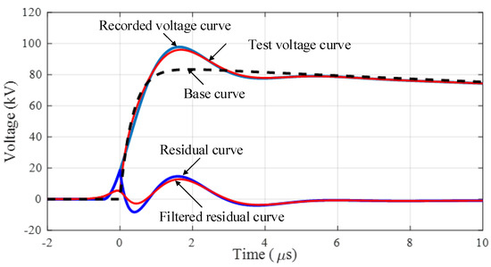 Figure 1. Voltage curves for determination of full lightning impulse voltage parameters.
- (2)
- From the digital waveform data, the offset voltage is determined and removed from the original recorded waveform. The waveform part utilized in the parameter determination ranges from the voltage of 20% of the waveform peak on the front section to 40% of the waveform peak on the tail section. The selected waveform is referred to as the recorded curve.
- (3)
- The base curve parameters in Equation (1) or Equation (2) (α, β, C, and td or A, B, α, and β) are determined by a curve fitting method. It is noted that in this paper the function in Equation (2) is selected as the base curve function for simplicity. The standards [1,2] recommend the Levenberg–Marquardt (LM) algorithm for the base curve parameter determination.
- (4)
- The difference of the recorded and base curves referred to as the residual curve is filtered by the k-factor function as given in Equation (3). The effective time domain implementation based on the IIR filter was proposed by P. L. Lewin [19].where f is the frequency in MHz.
- (5)
- The summation of the base and filtered residual curves referred to as the test voltage is utilized for the determination of the waveform parameters, i.e., T1, T2, Vp, and βe.
As mentioned in the introduction, the most crucial process of the parameter determination is the base curve fitting. The deficiency of the LM algorithm for the waveform parameter determination was found in cases of the high overshoot rate waveform. Many iterations and relatively long computational times lead to the method being improper in the waveform parameter determination. A non-iterative approach for determination of the base curve with promising accuracy is proposed in this paper. The original idea of the proposed method is an attempt for fitting the base curve by avoiding complicate and non-linear regression algorithms. The conventional separable exponential function fitting was further developed and the accuracy for the base curve parameter determination is increased. The details of the mentioned and proposed methods are presented in the following sections.
2.1. The Separable Exponential Function Fitting Method
The conventional separable exponential function fitting method [18] separates the recorded waveform into two parts, as illustrated in Figure 2. The first part of the waveform under consideration is the duration with which the overshoot and oscillation disappear from the waveform. Normally, this duration takes into account the time after the impulse voltage reaches the peak value. This instant is around two to three times of the time to peak. This part of the waveform can be fitted well with a single exponential function (Aeαt), and the logarithmic transformation and linear regression (LL) model can be used to determine the waveform parameters (A and α). The second part of the waveform is computed by subtracting the recorded waveform from the fitted waveform from the first part. Then, only the positive magnitude of the second part waveform is utilized for fitting with the LL model. As shown in Figure 3, it is found that the fitting parameters of this method are deviated from the results determined by the LM algorithm, but the integration method proposed in this paper provides the fitting curve closed to the LM method. It is noted that the integration method has the possibility of further development for the lightning waveform parameter evaluation. The derivation of the integration method will be presented in the next subsection.
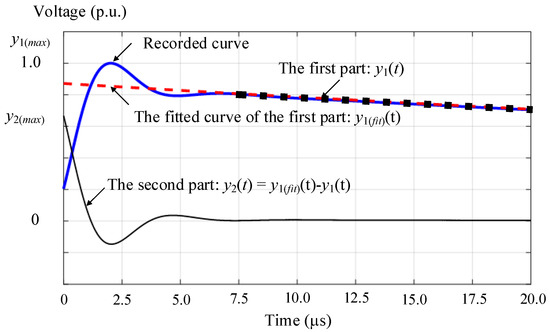
Figure 2.
Voltage curves for determination of full lightning impulse voltage parameters using the LL method.
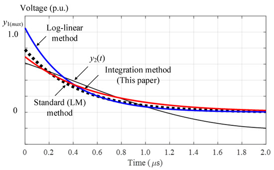
Figure 3.
Comparison of the fitting curve methods (LL, LM, and integration).
2.2. The Proposed Curve Fitting Method
The proposed method originated from the separable exponential fitting method, but the integration method is utilized for fitting the waveform instead of the LL method. Additionally, the precomputed correction models of the base curve parameters to those determined by the standard recommended method were developed. The procedures for determination of the full lightning impulse voltage parameters are the same as the standard recommended method, except the base curve determination.
In the proposed method, the data of 29 cases (LI-A1 to LI-A12 and LI-M1 to LI-M17) provided by the standard [13] were used for the model development. The vertical resolution and the sampling frequency of the waveforms were set to be 12 bits and 100 Msample/s, respectively. The normalized recorded curve (y1(t)), as shown in Figure 4, is employed to determine the base curve parameters. The base curve is defined by two terms of the exponential functions (Aeαt and Beβt). The curve duration from the time to peak (tp) to 40% of Vp on the tail section is utilized in a simple linear curve fitting for the determination of the first term which is in the form of a single exponential function (f1(t) = Aeαt).
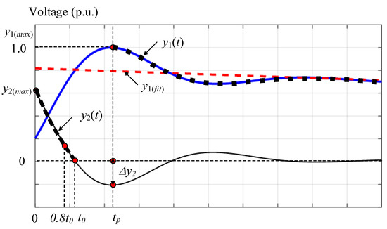
Figure 4.
Voltage curves used for the determination of the waveform parameters in the proposed method.
It was noticed that this first term is a solution of the first order differential equation as given in Equation (4).
Taking the integration of Equation (4) and rearranging the equation, the results are obtained as Equation (5).
From Equation (5), a linear regression can be applied to determine the coefficients of C and α. The coefficient of A in the first term can be calculated by Equation (6).
It was found that the proposed linear regression method provides the different results deviated from the results computed by the standard recommended (LM) method. The higher the undershoot factor (Δy2), the higher the deviations of the parameters (ΔA and Δα), as shown in Figure 5 and Figure 6.
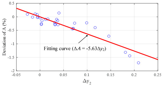
Figure 5.
Deviation of A versus the undershoot factor (Δy2) and the fitted curve.
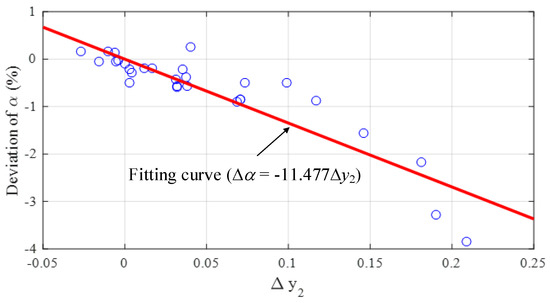
Figure 6.
Deviation of α versus the undershoot factor (Δy2) and the fitted curve.
The deviations (Δx) of the base curve parameters (A, B, α, or β) are defined as Equation (7), where xcal and xstd are the parameters computed by the proposed and standard recommended methods, respectively.
As given in Equations (8) and (9), the correction factors are applied to obtain the accurate results of the first term parameters (Acor and αcor).
These correction factors are calculated by the linear curve fitting, as shown in Figure 5 and Figure 6. With these correction factors, the deviations of the corrected parameters are within 1% and 2% for A and α, respectively.
For the second term of the exponential functions, the curve of y2(t) is computed by subtracting y1(t) from the corrected f1(t). It was found that using the waveform part with the only positive magnitude, the determined parameters (B and β) have good linear correlation with the undershoot factor (Δy2). For the reduction of the deviation of such a parameter in good linear relation with Δy2, the curve duration of y2(t) from 0 to t0 is employed to determine the second-term parameters of the base curve in the form of a single exponential function (f2(t) = Beβt), in cases of Δy2 over 1.5%. In cases of Δy2 below 1.5%, the curve duration of y2(t) from 0 to 0.8 t0 is employed to determine the base curve parameters. The second-term parameters can be determined by linear regression, as expressed in Equation (10), which is the same approach used for the first-term parameter determination. B and β also have good relations with the undershoot factor (Δy2). The deviations of B and β (ΔB and Δβ), the fitting curves, and their expression are presented in Figure 7 and Figure 8.
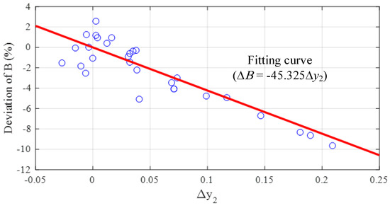
Figure 7.
Deviation of B versus the undershoot factor (Δy2).
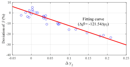
Figure 8.
Deviation of β versus the undershoot factor (Δy2).
As given in Equations (11) and (12), the correction factors for B and β are applied to obtain the accurate results of the second term parameters (Bcor and βcor). These correction factors are calculated by the linear curve fitting, as shown in Figure 7 and Figure 8. With the application of these correction factors, the deviations of the corrected parameters are within 3% and 6% for B and β, respectively.
Using the corrected base curve parameters, the base curve can be determined precisely. The full lightning impulse voltage waveform parameters (T1, T2, Vp, and βe.) can be determined by the procedures (4) and (5) of the standard recommended method [1,2]. The performances of the proposed method for the determination of the full lightning impulse voltage parameters will be investigated in the next section.
3. Validation of the Proposed Method
For the verification of the performance of the proposed method, impulse waveforms with various waveform parameters, i.e., front time (T1), time to half (T2), peak voltage (Vp), and overshoot rate (βe) were utilized in the waveform parameter determination. Such waveforms are composed of 29 waveform data (LI-A1 to LI-A12 and LI-M1 to LI-M17) from the test data generator (TDG) provided by IEC 61083-2 [13] and 10 additional waveform data (LI-X1 to LI-X10) collected from simulations and experiments. The determined waveform parameters and the deviations are presented in Table 1. The deviations are defined as the differences between the parameters determined by the proposed method and the values provided by the standard [13] (in the cases of the waveforms provided by the standard) or the differences from the values computed by the standard recommended method (in the cases of LI-X1 to LI-X10).

Table 1.
The determined waveform parameters using the proposed method and the deviations from the standard recommended values or the values computed using the standard recommended method.
According to the standard [13], the tolerances of the waveform parameters (T1, T2, Vp, and βe) are ±2%, ±1%, ±0.1%, and ±1%, respectively. It was found that all waveform parameters determined by the proposed method are within the standard defined tolerance. The maximum deviation of T1 computed by the proposed method is +1.6%, which occurs in the case of LI-M6. The maximum deviation of T2 is 0.1%, in the case of LI-M16. The maximum deviation of Vp is 0.07%, in the case of LI-X9 from an experiment. Additionally, the maximum deviation of βe is 0.41%, in the case of LI-X5 from an experiment. It has been shown that the proposed method used for the waveform parameter determination is fairly precise. Figure 9, Figure 10, Figure 11, Figure 12 and Figure 13 present the example waveforms assessed by the proposed method.
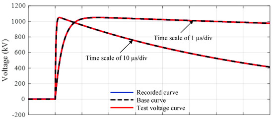
Figure 9.
The assessed full lightning impulse waveforms in the LI-A1 case (waveform data provided by [13]).
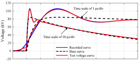
Figure 10.
The assessed full lightning impulse waveforms in the LI-A7 case (waveform data provided by [13]).
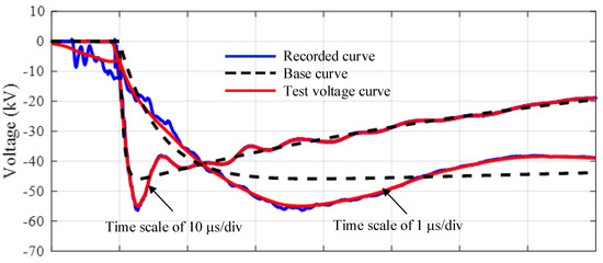
Figure 11.
The assessed full lightning impulse waveforms in the LI-M5 case (waveform data provided by [13]).
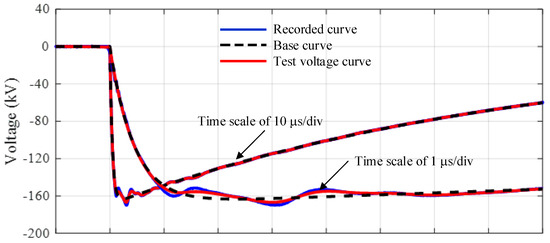
Figure 12.
The assessed full lightning impulse waveforms in the LI-M6 case (waveform data provided by [13]).
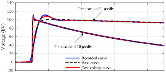
Figure 13.
The assessed full lightning impulse waveforms in the LI-X9 case (experimental waveform data).
In addition, comparisons of the maximum deviation using the method proposed in this paper with the maximum deviation using other non-iterative methods (the double integration [16] and the improved Prony’s methods [17]) and the neural network-based method [18] as well as a developed software based on Matlab and the IEC procedure [1] are studied and presented in Table 2. It should be noted that only waveforms provided by the standard [13] are considered for comparisons, as shown in Table 2. Comparisons of the execution times used for the proposed method, the methods in [16,17,18], the IEC procedure [1], and the commercial software [20] are presented in Table 3. All methods and the commercial software were executed on the same computer with the CPU i5-4210U and 2.40 GHz. In comparison to the existing non-iterative and neural network-based methods, the proposed method provides superior accuracy in the determination of the waveform parameters. The execution times of the proposed method are nearly the same as those provided by the non-iterative methods and are significantly shorter than those provided by the commercial software.
Table 2.
The comparison of the maximum deviations of the waveform parameters determined by the proposed and other non-iterative methods.
Table 3.
The comparison of the execution times for the waveform parameters determined by the proposed and other non-iterative methods and the commercial software.
4. Conclusions
The simple, accurate, and non-iterative method based on the integration method with the precomputed correction model for fitting exponential functions has been proposed to determine the full lightning impulse voltage parameters in this paper. The waveform data from the standard, simulations, and experiments (39 cases in total) have been utilized in the assessment of the proposed method performances. It was found that the method displays promising performances in terms of accuracy and computation speed because there is no iteration requirement. All waveform parameters determined by the proposed method are within the tolerances defined by the standard. From the presented results it has been confirmed that the proposed method is fairly accurate and useful for the determination of the full lightning waveform parameters because the method is simple, has no iteration process, and is easy for software implementation in practical impulse voltage tests.
Funding
This research was funded by National Research Council of Thailand.
Institutional Review Board Statement
Not applicable.
Informed Consent Statement
Not applicable.
Data Availability Statement
Not applicable.
Acknowledgments
The authors would like to give special acknowledgement to the School of Engineering, King Mongkut’s Institute of Technology Ladkrabang, for providing the facilities for this research work and National Research Council of Thailand for financial support.
Conflicts of Interest
The authors declare no conflict of interest.
References
- IEC 60060-1. High-Voltage Test Techniques. Part 1: General Definitions and Test Requirements, 3rd ed.; IEC: Geneva, Switzerland, 2010. [Google Scholar]
- IEEE Standard 4TM-2013. IEEE Standard for High-Voltage Testing Techniques. In Proceedings of the Fall 2016 IEEE Switchgear Committee Meeting, Pittsburgh, PA, USA, 9–13 October 2016. [Google Scholar]
- Kuffel, E.; Zaengl, W.S.; Kuffel, J. High Voltage Engineering: Fundamentals, 2nd ed.; Newnes: Oxford, UK, 2000. [Google Scholar]
- Glaninger, P. Impulse testing of low inductance electrical equipment. In Proceedings of the 2nd International Symposium on High Voltage Technology, Zurich, Switzerland, 9–13 September 1975; pp. 140–144. [Google Scholar]
- Feser, K. Circuit design of impulse generators for the lightning impulse voltage testing of transformers, Haefely High Voltage Technology. Bull. SEV/VSE Bd 1977, 68. Available online: www.haefely.com (accessed on 15 November 2019).
- Schrader, W.; Schufft, W. Impulse voltage test of power transformers. In Proceedings of the Workshop 2000, Alexandria, VA, USA, 13–14 September 2000. [Google Scholar]
- Karthikeyan, B.; Rajesh, R.; Balasubramanian, M.; Saravanan, S. Experimental Investigations on IEC Suggested Methods for Improving Waveshape During Impulse Voltage Testing. In Proceedings of the 2006 IEEE 8th International Conference on Properties & applications of Dielectric Materials, Bali, Indonesia, 26–30 June 2006. [Google Scholar]
- Tuethong, P.; Kitwattana, K.; Yutthagowith, P.; Kunakorn, A. An algorithm for circuit parameter Identification in lightning Impulse voltage generation for low-inductance loads. Energies 2020, 13, 3913. [Google Scholar] [CrossRef]
- Mirzaei, H.R. A Simple Fast and Accurate Simulation Method for Power Transformer Lightning Impulse Test. IEEE Trans. Power Deliv. 2019, 34, 1151–1160. [Google Scholar] [CrossRef]
- Mirzaei, H.; Bayat, F.; Miralikhani, K. A semi-analytic approach for determining Marx generator optimum set-up during power transformers factory test. IEEE Trans. Power Deliv. 2021, 36, 10–18. [Google Scholar] [CrossRef]
- Okabe, S.; Tsuboi, T.; Takami, J. Evaluation of Κ-factor based on insulation characteristics under non-standard lightning impulse waveforms. IEEE Trans. Dielectr. Electr. Insul. 2009, 16, 1124–1126. [Google Scholar] [CrossRef]
- Tsuboi, T.; Ueta, G.; Okabe, S.; Shimizu, Y.; Ishikura, T.; Hino, E. K-Factor Value and Front-Time-Related Characteristics in Negative Polarity Lightning Impulse Test for UHV-Class Air Insulation. IEEE Trans. Power Deliv. 2013, 28, 1148–1155. [Google Scholar] [CrossRef]
- IEC 61083-2. Instruments and Software Used for Measurement in High-Voltage and High Current Tests. Part 2: Requirements for Software for Tests with Impulse Voltages and Currents, 2nd ed.; IEC: Geneva, Switzerland, 2013. [Google Scholar]
- Jamroen, P.; Yoosorn, P.; Waengsothorn, S.; Yutthagowith, P. Modified Gauss–Newton algorithm for evaluation of full lightning impulse voltage parameters. Sens. Mater. 2021, 33, 2631. [Google Scholar] [CrossRef]
- Li, Y.; Kuffel, J.; Janischewskyj, W. Exponential fitting algorithms for digitally recorded HV impulse parameter evaluation. IEEE Trans. Power Deliv. 1993, 8, 1727–1735. [Google Scholar] [CrossRef]
- Pattanadech, N.; Yutthagowith, P. Fast curve fitting algorithm for parameter evaluation in lightning impulse test technique. IEEE Trans. Dielectr. Electr. Insul. 2015, 22, 2931–2936. [Google Scholar] [CrossRef]
- Yutthagowith, P.; Pattanadech, N. Improved Least-Square Prony Analysis Technique for Parameter Evaluation of Lightning ImpulseVoltage and Current. IEEE Trans. Power Deliv. 2016, 31, 271–277. [Google Scholar] [CrossRef]
- Yutthagowith, P.; Kitwattana, K.; Kunakorn, A. Fast and effective technique in evaluation of lightning impulse voltage parameters. J. Electr. Eng. Technol. 2020, 16, 459–467. [Google Scholar] [CrossRef]
- Lewin, P.L.; Tran, T.N.; Swaffield, D.J.; Hallstrom, J.K. Zero-Phase Filtering for Lightning Impulse Evaluation: A K-factor Filter for the Revision of IEC60060-1 and -2. IEEE Trans. Power Deliv. 2007, 23, 3–12. [Google Scholar] [CrossRef]
- User Manual for Digital Impulse Measuring Systems, Transient Recorders and Evaluating Systems, Downloaded in Jan. 2022. Available online: http://www.strauss-mess.de/dokumente/WinTRAS-KAL-E.pdf (accessed on 8 January 2022).
Publisher’s Note: MDPI stays neutral with regard to jurisdictional claims in published maps and institutional affiliations. |
© 2022 by the author. Licensee MDPI, Basel, Switzerland. This article is an open access article distributed under the terms and conditions of the Creative Commons Attribution (CC BY) license (https://creativecommons.org/licenses/by/4.0/).