A Hybrid AOSAOA Scheme Based on the Optimal Location for Electric Vehicle Parking Lots and Capacitors in a Grid to Care of Voltage Profile and Power Loss

Abstract

In this manuscript, a hybrid system depending on the optimal location of electric vehicle parking lots (PL) and capacitors under voltage profile care and power loss is proposed. The proposed hybrid scheme is the joint execution of both the atomic orbital search (AOS) and arithmetic optimization algorithm (AOA). Commonly it is called the AOSAOA technique. In the paper, the allocation of the parking lot and capacitor is introduced to congestion management with reactive power compensation. To optimally regulate that parking lot size, the AOSAOA technique is adopted. Furthermore, parking lot and capacitor allocation are introduced to congestion management and reactive power compensation. With this proper control, the perfect sitting of capacitor and EV parking lots under the grid, including the deterioration of real and reactive power loss and voltage profiles are optimally chosen. Furthermore, the implementation of the proposed AOSAOA model is developed by the MATLAB/Simulink platform, and the efficiency of the proposed model is likened to other techniques.

1. Introduction

Today, in countries that rely heavily on imported crude oil, key anxieties regarding climate change and increasing oil prices have pushed energy efficiency to become a basic standard. At present, the transportation sector accepts a large part of oil consumption, a large part of which is utilized for road vehicles [1]. As a result, oil prices are rising day by day, bringing burdens to the lives of ordinary people. With the protection of energy and the environment, the worldwide focus in the future will be on alternative transportation, such as electric vehicles (EV) [2]. The invention of rechargeable batteries was applied to electric vehicles that used electric motors and distributed electricity in the 19th century. By charging the battery when necessary, people will feel comfortable driving such electric cars in the city. The top probable position also allows the frame to alleviate voltage problems at different nodes while reducing current leakage from capacitive components. With the increasing popularity of electric vehicles [3], it is necessary to improve the charging infrastructure and provide new affordable models. Since cleaner solutions help people live in a healthy environment, the government provides incentives acceptance of electric vehicles and prolongs investment in infrastructure [4].

Today, electric vehicles have become the hopeful option of powered motor vehicles for general transportation, so charging points need to expand locally in the future. Electric vehicles will be related through a power distribution network that uses charging stations. According to [4], a multi objective optimization method is implemented for modeling difficult assignments. However, in [4], the authors considered the vehicle-to-grid (V2G) under its work but they did not consider the impact of the use of electric vehicles on congestion management. Furthermore, in [5], the allocation of electric vehicle parking was proposed with a detailed probability model of EVPL on the distribution network. In [6], a parking-based allocation system was utilized to catch the best parking location in the Nordic region. Additionally, the impact of EVPL demand on power distribution network losses was studied in depth in [7]. In [8], the restricted distribution of the electric vehicle distribution network was studied. In [9], GA and particle swarms were used to perform the reliability-driven distribution optimization (PSO) of electric vehicle charging points. In [10], the authors proposed a comparable work. A loading system was recommended in [11] to change the maximum load to off-peak hours. Regarding the problems of voltage violation and minimizing power loss, dissimilar load plans are expected. S. Pazouki et al. [12] proposed the simultaneous optimal planning (placing and sizing) of charging stations and distributed generations to address new challenges. They used a genetic algorithm for a simulation study on a 33-bus radial distribution network. The simulation results show the effects of the installation of charging stations in the presence/absence of distributed generations on total costs, reliability, loss, voltage profile, and emission. K. Karmaker et al. [13] proposed an electric vehicle charging station (EVCS) based on solar and biogas to reduce the burden on the national grid. This proposed EVCS integrates a combination of a solar PV module, three biogas generators, 25 lead-acid batteries, a converter, and charging assemblies. They analyzed the economic, technical, and environmental feasibility of the proposed EVCS using Hybrid Optimization of Multiple Energy Renewable Pro software [14]. This proposed method was investigated on a 33-bus system to validate the optimal sitting and sizing of RES and EV charging stations simultaneously. M. Atwa et al. [15] proposed a methodology for the optimal allocation of different types of renewable distributed generation units to reduce annual energy loss in the distribution system.

India and other developing economies have also adopted these collection strategies. J. Teng et al. [16] designed optimal charging/discharging scheduling for battery storage systems (BSSs) that minimizes the distribution systems’ losses. Using the genetic algorithm-based method, the results demonstrated the validity of the proposed mathematical model and optimal charging/discharging schedule. M. Mazidi et al. [17] proposed a method in which the reserve requirement for compensating renewable forecast errors was provided by both responsive loads and distributed generation units. The reserve requirement for compensating renewable forecast errors was provided by both responsive loads and distributed generation units. J. GeunKim and M. Kuby [18] developed a linear programming model for optimizing the locations of refueling stations by considering a vehicle’s driving range and the necessary deviations of drivers. It shows the maximization of total flows refueled on deviation paths and the decrease of the captured demand flows with an increase in deviation distances, which led to the fragmentation of the global auto market, such as India and Southeast Asia. Two- and three-wheelers are attractive short-term targets. In China, Europe, the United States, and the rest of the world, it is closely followed due to active government measures and continues to lead electric vehicles across the board. It can be clearly seen from the literature review that the distribution grid voltage curve is kept within limits by the smart charging of electric vehicles. V2G apps have yet to do that job. Using the best location for electric vehicle parking lots, it turns out that execution does not rely solely on incentives. Therefore, economically and the geologically convenient charge is a must, as are homes, shopping malls, workplaces, and charging station parking lots. The key feature implies the time variable that consumers value the most. The loss can also be reduced using multiple generators. 22Kmeans clustering technology was abandoned to analyze the best PL citations at the same time that the ECCRP mathematical formula was described, and a probability-based method was developed to optimize EVPL appointment and size [19]. All CS designs, as a planning model for the distribution network overlay, are concerned with the optimal configuration of CS under the overlay grid. The current work attempts to propose [20] a classification that outlines certain planning models for difficult CS placement as the overlap of the distribution.

2. Recent Research Work: A Brief Review

In the literature, based on the use of various technologies and aspects of the optimal configuration of electric vehicle charging points, various research works can be carried out. Some of them seek feedback: S. Sachan et al. [21] proposed a new method of occasionally charging electric vehicles. In the study, it is recommended to allocate parking lots and condensers congestion management and reactive power compensation. To do this, they performed an analysis by assessing the inverse Jacobian matrix of current research. Biogeography-based optimization technology is used to optimize parking lot size. The expected technology effectiveness was tested on a custom IEEE 34-bus distribution network. Surbhi Aggarwal and Amit Kumar Singh [22] studied the installation of rapid charging stations, a case study on a 24-bus system. This work demonstrates the location of charging stations through dissimilar nominal powers of 5, 25, 50, and 100 MW in different systems of test cases on the load bus line, taking into account the violation of the voltage amplitude limits (0.95 < V < 1.05) ratings. Appropriate site selection and size adjustments were made for the DG, and four different test cases were considered, among which charging stations were pre-installed to overcome network loss and maintain system stability. Mohd Bilal and Mohammad Rizwan [23] demonstrated a new hybrid technology to study the best location for electric vehicle charging stations. In addition, this article performs a thorough inspection of the vehicle’s facilities to the network. The proposed hybrid method contains Particle Swarm Optimization and Hybrid Gray Wolf Optimization. With the mix of these algorithms of ideal properties and development capabilities, M. Ahmadi et al. [24] proposed the difficulty of the optimal allocation of parking lots of electric vehicles and programming of the optimal operation of electric vehicles under an intelligent distribution network. Different factors involving technical and economic aspects were considered in the questions posed to achieve real solutions. In terms of technical issues, it was considered to lessen network losses and lessen voltage drop between feeders, as well as meet network requirements wholly. In addition, in the questions posed, the total cost of purchasing power and the total cost of loading and unloading the electric vehicle parking lots around the Pearl River Delta was considered based on price.

L. Chen et al. [25] proposed an electric vehicle charging station (EVCS) and explained a new optimized allocation and size adjustment under the Allahabad power distribution system in India. Their key impression considers the reduction in reactive power loss index, improvement in voltage power index, reduction in actual power loss index, and initial cost to optimize EVCS configuration to obtain the smallest installation. To solve the nonlinear optimization mixed-integer difficulty, a new meta-heuristic algorithm is proposed, called the balanced Mayfly algorithm. The modification is to improve precision and solve the problem of algorithm scanning. Charles Raja S [26] demonstrated a two-layer hybrid programming method that improves system reliability using optimizing vehicle charging stations (VCS) that integrate plug-in hybrid electric vehicles and renewable distributed power generation (RDG) at the same time. In the presence of RDG volatility, there are extensive requirements among customers to ensure continuity of supply. Therefore, based on various emergency analyses, a non-linear objective function was developed to lessen the lack of power supply (ENS) provided to customers. Two notable contributions stand out from existing efforts. First, identify the best location for selecting both the RDG and the charging station. Considering the simultaneous integration of VCS and RDG, a method based on the hybrid Nelder Mead Cuckoo Search algorithm is adopted to minimize ENS, smoothly reduce power loss, and increase the voltage range in the system. P. Rajesh and F.H. Shajin [27] proposed an innovative method for charging stations (CS) with optimal planning and capacitors in the new technology. To accomplish a better balance between the exploration and development of the Dragonfly (DA) algorithm, Gaussian and quantum mutation strategies are used in DA performance. This is the novelty of the work we have shown. Therefore, it is called the quantum effect Gaussian mutation Dragonfly Algorithm. Here, this algorithm is recommended to allocate parking spaces and capacitors and reactive power compensation for congestion management.

Background of Research Work

A review of current research work portrays the optimal configuration of charging stations of an electric vehicle as an important influencing factor. With the quick expansion of EV charging technology, numerous charging facilities are being used at electric vehicle charging stations (EVCS). Charging through dissimilar charging powers may meet the charging needs of different electric vehicles and affect the temporal at the same time and spatial distribution of electric vehicle charging requirements, posing challenges to the rationality and economics of the EVCS allocation plan. To improve the charging efficiency of electric vehicles and alleviate the aforementioned pain points, optimal EVCS planning is becoming an extremely important issue. The optimized configuration scheme of EVCS can meet the charging needs of different electric vehicle owners at the minimum social cost, thus promoting the development of the electric vehicle industry. Genetic Algorithms (GA), Heuristic algorithms, Particle Swarm Optimization (PSO), GAPSO Hybrid Algorithm, and Chemical Reaction Optimization, in addition to Differential Evolution (DE), are techniques commonly used. In addition, the optimization model with a linear integer is utilized to regulate the location of the EVCS and is competently resolved through an optimization solver. Furthermore, in real life, EVCS always mixes and installs multiple charging facilities to meet diversified charging needs. This phenomenon complicates the electric vehicle charging needs, which is why it is great to seek an efficient method to optimize the planning of electric vehicles with multiple charging facilities. These above-mentioned shortcomings are produced in the existing system that carries on this research work.

3. System Modeling of EV

In this article, we consider a smart grid that powers commercial consumers. These buildings are equipped with wind energy and photovoltaic units related to the grid. In addition, electric vehicle charging stations have been set up in the parking area of the workplace and are powered by photovoltaic and wind generators. The goal of the proposed system is to measure the optimal size of electric vehicle parking lots and capacitors on the power distribution system. When the load suddenly has a high demand, the DC bus capacitor is located on the DC side to stabilize the DC bus voltage. An overview of the electric vehicle parking lot (PL) based on the proposed approach is shown in Figure 1. The major part of the electric vehicle charging station (EVCS) is the DC bus, where all the electric vehicles (EVs) are situated for charging. The modeling and mathematical formulations of the sources are described as follows.

3.1. Modeling of EV

The vehicle model includes a driver, vehicle dynamics, and a power system. A driver’s model with input is the actual vehicle speed compared to the reference speed. The output of the driver model is the positions of the brake pedal and the accelerator pedal. The power system receives the instruction from the driver’s pedal position and fulfills it through EM and ICE.

The combined active power of the internal combustion engine (ICE) and energy management (EM) acts as a result of the power system and input model of the vehicle’s dynamics, namely drag, force, traction, rolling resistance, and gravitational force presented by the slopes of the road [28]. Figure 1 show an overview of an EVCS with parking spaces. The deviation of EV is estimated based on Equation (1)

$$E{V}_d(t)=\frac{1}{{\sigma }^{\ast }\sqrt{2\mathsf{\Pi }}}{e}^{-(t-{\mu }^{\ast })/2{\sigma }^{\ast }{}^2},0<t<24$$

(1)

where ${\sigma }^{\ast }$ is the standard deviation and its value is 3.1, and ${\mu }^{\ast }$ is the mean value and its value is 16.97. The arrival of the EV is estimated based on Equation (2)

$$E{V}_a(t)=\frac{1}{{\sigma }^{\ast }\sqrt{2\mathsf{\Pi }}}{e}^{-(t-{\mu }^{\ast })/2{\sigma }^{\ast }{}^2},0<t<24$$

(2)

where the value of ${\mu }^{\ast }$ and ${\sigma }^{\ast }$ are 17.01 and 3.2. The EV distance is estimated using the following Equation (3).

$$E{V}_d(d)=\frac{1}{d{\sigma }^{\ast }\sqrt{2\mathsf{\Pi }}}{e}^{-(\ln d-{\mu }^{\ast })/2{\sigma }^{\ast }{}^2},d>0$$

(3)

Here, $d$ shows the travel distance and the values of ${\mu }^{\ast }$ and ${\sigma }^{\ast }$ are 3.2 and 0.9.

3.2. Mathematical Formulation of PV System

Solar cells are basic elements for generating PV systems. Solar cells are coupled in series or in parallel to create a solar cell matrix with the required rating. Figure 2 show the circuit of the solar energy system. In the photovoltaic energy subsystem, sunlight stored with a solar power panel becomes electrical energy [29]. Y. Song, Y. Zheng, and D. Hill (2016) proposed a convexified model, converted using convex relaxation techniques from the conventional model [30], which is applied for 15-bus distribution networks and reduces the total energy and charging cost. In this model, high computational efficiency and optimal solution can be achieved [31]. S. Fazeli, S. Venkatachalam, R. Chinnam, and A. Murat (2020) proposed an embedded two-stage stochastic model which determines the types of EV supply and optimal layout [32]. H. Zhang et al. developed an algorithm using a Gaussian operator and mixed an algorithm for different variations. These algorithms are applied in practical locating planning projects and reduce social costs [33]. L. Gong et al. proposed an optimal charging technique based on a dynamic spike pricing policy with distribution transformer normal operation for reducing the charging cost. They used a genetic algorithm (GA) to reduce charging costs with effective peak sharing [34]. Using Equation (4), the power generated through the photovoltaic system was calculated

$$P_{pv}=R_t{\eta }_{pv}{A}_{pv}$$

(4)

where $P_{pv}$ represents the power output of the photovoltaic panel, $R_t$ represents the solar radiation in the inclined plane module, ${\eta }_{pv}$ represents the efficiency of the photovoltaic panel, and $A_{pv}$ is the area of the photovoltaic panel. The following Equation (5) clarifies the efficiency of photovoltaic panels,

$${\eta }_{pv}={\eta }_{r-pv}{\eta }_{PC}\left[1-N_T\left(T_C-T_{ref}\right)\right]$$

(5)

where photovoltaic panel implies ${\eta }_{pv}$, reference module implies ${\eta }_{r-pv}$, power condition implies ${\eta }_{PC}$, photovoltaic panel temperature coefficient denotes $N_T$, cell temperature (°C) implies $T_C$ as in Equation (6), and the cell temperature on reference conditions is $T_{ref}$. Likewise, $T_{ref}$ is placed through 25 °C and takes on $N_T$’s value of −3.7 × 10⁻³ °C⁻¹ for the temperature of mono and poly crystalline silicon.

$$T_C=T_A+\left[\frac{NOCT-20}{800}\right]R_t$$

(6)

where, $T_A$ implies temperature of ambient air and $NOCT$ implies nominal cell operating temperature.

The PV module current is articulated as Equation (7)

$$I^{\ast }=I_L^{\ast }-I_{sat}^{\ast }\left[\exp \left\{q^{\ast }\frac{V_{pv}^{\ast }+I_{pv}^{\ast }·R_s^{\ast }}{\upsilon k{T}_c}\right\}-1\right]-\frac{V_{pv}^{\ast }+I_{pv}^{\ast }·R_s^{\ast }}{R_{sh}^{\ast }}$$

(7)

where $I_L^{\ast }$ signifies the created current for Light A, $R_{sh}^{\ast }$ and $R_s^{\ast }$ are series and shunt resistances in Ω, $k$ represents Boltzmann’s constant, $\upsilon$ signifies the ideal factor of p-n, $V_{pv}^{\ast }$ and $I_{pv}^{\ast }$ are the solar cell output voltage and current, and $I_{sat}^{\ast }$ indicates the reverse saturation current in A. $I_{sat}^{\ast }$ shows the reverse saturation current and $I_L^{\ast }$ shows the light-generated current illustrated in Equations (8) and (9)

$$I_L^{\ast }=\left[I_{sc}+\gamma (T_c-T_c^{\ast })\right]\frac{C_T}{C_T^{\ast }}$$

(8)

$$I_{sat}^{\ast }=\frac{I_{sc}\gamma (T_c-T_c^{\ast })}{\exp \left[\frac{V_{oc}\gamma (T_c-T_c^{\ast })}{V_T}\right]-1}$$

(9)

where $T_c$ are the PV cell’s ambient temperature, $C_T$ implies irradiance, $\gamma$ is the temperature coefficient under short circuit current, $V_T$ is the thermal voltage, and $V_{oc}$ is the open-circuit voltage at standard temperature.

3.3. Modeling of Parking Lot and Capacitor

Electric vehicle charging infrastructure plays a very important role in electric vehicle parking locations, including capacitors, because in electric vehicle parking, as active power loss reduces, system performance improves reliability and efficiency. Charging infrastructure includes all the tools and procedures used to transfer electricity from the grid to the vehicle. A charging area with an acceptable charging time system can improve the performance of electric vehicles and reduce public charging requirements. The following Equation (10) shows the power loss.

$$P_L^{\ast }={\displaystyle \sum _{i,j=1}^n\left[{\upsilon }_{ij}(P_i^{\ast }{P}_j^{\ast }+Q_i^{\ast }{Q}_j^{\ast })+{\varsigma }_{ij}(Q_i^{\ast }{P}_j^{\ast }-P_i^{\ast }{Q}_j^{\ast })\right]}$$

(10)

Here, $P_i^{\ast }$ and $Q_i^{\ast }$ specifythat bus $i$ is active and has reactive power injections, $P_j^{\ast }$ and $Q_j^{\ast }$ implicate that bus $j$ is active with reactive power injections, and $n$ denotes the number of buses. The ${\upsilon }_{ij}$ and ${\varsigma }_{ij}$ can be expressed by (11)

$${\upsilon }_{ij}=\left(\frac{x_{ij}}{V_i^{\ast }{V}_j^{\ast }}\right)\cos ({\beta }_i-{\beta }_j)$$

(11)

$${\varsigma }_{ij}=\left(\frac{x_{ij}}{V_i^{\ast }{V}_j^{\ast }}\right)\sin ({\beta }_i-{\beta }_j).$$

(12)

Here, the voltage of buses i and j is shown as $V_i$ and $V_j$, the bus admittance matrix is represented as $Y_{ij}$, the load angles of buses i and j are ${\beta }_i$ and ${\beta }_j$, ${\varsigma }_{ii}$ and ${\upsilon }_{ii}$ are the susceptance and conductance values, N is thenumber of buses. Where, $V_i^{\ast }$ and $V_j^{\ast }$ imply $i$ and $j$ bus voltage and $x_{ij}$ denotes the impedance matrix.

$$\frac{\partial P_L^{\ast }}{\partial P_i^{\ast }}=2{\upsilon }_{ii}{P}_i^{\ast }+2{\displaystyle \sum _{\begin{array}{l}j\ne i\\ j=1\end{array}}^n\left({\upsilon }_{ij}{P}_j^{\ast }-{\varsigma }_{ij}{Q}_j^{\ast }\right)}=0$$

(13)

$$P_i^{\ast }=-\frac{1}{{\upsilon }_{ii}}\left[{\displaystyle \sum _{\begin{array}{l}j\ne i\\ j=1\end{array}}^n\left({\upsilon }_{ij}{P}_j^{\ast }-{\varsigma }_{ij}{Q}_j^{\ast }\right)}\right]$$

(14)

Also

$$P_i^{\ast }=P_i^{\ast EV}+P_{Gi}^{\ast }-P_{Di}^{\ast }$$

(15)

The EVs, PL size, and the size of the capacitor are presented in Equations (16) and (17).

$$P_i^{\ast EV}=P_{Di}^{\ast }-P_{Gi}^{\ast }-\frac{1}{{\upsilon }_{ii}}\left[{\displaystyle \sum _{\begin{array}{l}j\ne i\\ j=1\end{array}}^n\left({\upsilon }_{ij}{P}_j^{\ast }-{\varsigma }_{ij}{Q}_j^{\ast }\right)}\right]$$

(16)

$$Q_i^{\ast EV}=Q_{Di}^{\ast }-Q_{Gi}^{\ast }-\frac{1}{{\upsilon }_{ii}}\left[{\displaystyle \sum _{\begin{array}{l}j\ne i\\ j=1\end{array}}^n\left({\upsilon }_{ij}{Q}_j^{\ast }+{\varsigma }_{ij}{P}_j^{\ast }\right)}\right]$$

(17)

where $P_{Gi}^{\ast }$ implies the grid power in bus i and $P_{Di}^{\ast }$ specifies bus I power demand. The active and reactive power of bus $i$ and $j$ are estimated using Equations (18) and (19).

$$P_i^{\ast }=V_i^{\ast 2}{G}_{ii}^{\ast }+{\displaystyle \sum _{\frac{j=1}{j\ne 1}}^n\left|V_i^{\ast }{V}_j^{\ast }{Y}_{ij}\right|}\cos \left({\theta }_{ij}^{}-{\beta }_i^{}+{\beta }_j^{}\right)$$

(18)

$$Q_i^{\ast }=-V_i^{\ast 2}{B}_{ii}^{\ast }-{\displaystyle \sum _{\frac{j=1}{j\ne 1}}^n\left|V_i^{\ast }{V}_j^{\ast }{Y}_{ij}\right|}\sin \left({\theta }_{ij}^{}-{\beta }_i^{}+{\beta }_j^{}\right).$$

(19)

Here, $P_i^{\ast }$ implies the bus i active power and $Q_i^{\ast }$ implies the bus i reactive power. Where $G_{ii}^{\ast }$ implies the conductance of bus $i$, ${\theta }_{ij}^{}$ implies the angle magnitude of self-admittance at line $i$ to $j$ and $B_{ii}^{\ast }$ implies the susceptance at bus $i$. The indexes of sensitivity in the form of the voltage angles and magnitudes are illustrated by

$$\left[\begin{array}{l}\Delta P_{}^{\ast }\\ \Delta Q_{}^{\ast }\end{array}\right]=\left[\begin{array}{l}{J}_{11}^{\ast }{J}_{12}^{\ast }\\ J_{21}^{\ast }{J}_{22}^{\ast }\end{array}\right]\left[\begin{array}{l}\Delta \beta \\ \Delta V\end{array}\right]$$

(20)

$$\left[\begin{array}{l}\Delta \beta \\ \Delta V\end{array}\right]=\left[\begin{array}{l}{U}_1^{\ast }{U}_2^{\ast }\\ U_3^{\ast }{U}_4^{\ast }\end{array}\right]\left[\begin{array}{l}\Delta P_{}^{\ast }\\ \Delta Q_{}^{\ast }\end{array}\right].$$

(21)

$\Delta P_{}^{\ast }$ is denoted as active power deviation, $\Delta Q_{}^{\ast }$ is represented as reactive power deviation, $\Delta V$ signifies the voltage deviation, $\Delta \beta$ denotes the deviation of load angles of bus i and bus j as ${\beta }_i$ and ${\beta }_j$ where, $J_{}^{\ast }$ shows matrices and $U_1^{\ast }$, $U_2^{\ast }$, $U_3^{\ast }$, and $U_4^{\ast }$ are the voltage variation impacts regarding power on every distribution network bus which is illustrated by the following Equations (22)–(25).

$$U_1^{\ast }=\left[\begin{array}{cccc}\frac{\partial {\beta }_2}{\partial P_2^{\ast }}& \frac{\partial {\beta }_2}{\partial P_3^{\ast }}& \dots & \frac{\partial {\beta }_2}{\partial P_n^{\ast }}\\ .& .& .& .\\ .& .& .& .\\ \frac{\partial {\beta }_n}{\partial P_2^{\ast }}& \frac{\partial {\beta }_n}{\partial P_3^{\ast }}& \dots & \frac{\partial {\beta }_n}{\partial P_n^{\ast }}\end{array}\right]$$

(22)

$$U_2^{\ast }=\left[\begin{array}{cccc}\frac{\partial {\beta }_2}{\partial Q_2^{\ast }}& \frac{\partial {\beta }_2}{\partial Q_3^{\ast }}& \dots & \frac{\partial {\beta }_2}{\partial Q_n^{\ast }}\\ .& .& .& .\\ .& .& .& .\\ \frac{\partial {\beta }_n}{\partial Q_2^{\ast }}& \frac{\partial {\beta }_n}{\partial Q_3^{\ast }}& \dots & \frac{\partial {\beta }_n}{\partial Q_n^{\ast }}\end{array}\right]$$

(23)

$$U_3^{\ast }=\left[\begin{array}{cccc}\frac{\partial V_2^{\ast }}{\partial P_2^{\ast }}& \frac{{\partial }_2^{\ast }{V}_2^{\ast }}{\partial P_3^{\ast }}& \dots & \frac{\partial V_2^{\ast }}{\partial P_n^{\ast }}\\ .& .& .& .\\ .& .& .& .\\ \frac{\partial V_n^{\ast }}{\partial P_2^{\ast }}& \frac{\partial V_n^{\ast }}{\partial P_3^{\ast }}& \dots & \frac{\partial V_n^{\ast }}{\partial P_n^{\ast }}\end{array}\right]$$

(24)

$$U_4^{\ast }=\left[\begin{array}{cccc}\frac{\partial V_2^{\ast }}{\partial Q_2^{\ast }}& \frac{\partial V_2^{\ast }}{\partial Q_3^{\ast }}& \dots & \frac{\partial V_2^{\ast }}{\partial Q_n^{\ast }}\\ .& .& .& .\\ .& .& .& .\\ \frac{\partial V_n^{\ast }}{\partial Q_2^{\ast }}& \frac{\partial V_n^{\ast }}{\partial Q_3^{\ast }}& \dots & \frac{\partial V_n^{\ast }}{\partial Q_n^{\ast }}\end{array}\right]$$

(25)

After that, the subsequent four sensitivity indexes are denoted in Equations (26)–(29).

$$I_{1i}^{\ast }=\frac{{\displaystyle \sum _{k=1}^n\frac{\partial {\beta }_k}{\partial P_i^{\ast }}}}{N}$$

(26)

$$I_{2i}^{\ast }=\frac{{\displaystyle \sum _{k=1}^n\frac{\partial V_k^{\ast }}{\partial P_i^{\ast }}}}{N}$$

(27)

$$I_{3i}^{\ast }=\frac{{\displaystyle \sum _{k=1}^n\frac{\partial {\beta }_k}{\partial Q_i^{\ast }}}}{N}$$

(28)

$$I_{4i}^{\ast }=\frac{{\displaystyle \sum _{k=1}^n\frac{\partial V_k^{\ast }}{\partial Q_i^{\ast }}}}{N}$$

(29)

Here, $I_{1i}^{\ast }$ denotes the current in the first bus, $I_{2i}^{\ast }$ represents the current in the second bus, $I_{3i}^{\ast }$ denotes the current in the third bus, $I_{4i}^{\ast }$ represents the current in the fourth bus, and $N$ denotes the count of distribution network nodes. The active and reactive power flow among the nodes is indicated via the factor of contribution from the electric vehicle parking lot, including the capacitor. Rated power amid bus $i$ and bus $j$ is demonstrated using the following Equations (30) and (31).

$$P_{ij}^{\ast }=P_{ij}^{\ast b}+\Delta P_{ij}^{\ast }$$

(30)

$$\Delta P_{ij}^{\ast }={\displaystyle \sum _{N=1}^{Nb}\frac{\partial P_{ij}^{\ast }}{P_N^{\ast EV}}}\Delta P_N^{\ast }+{\displaystyle \sum _{N=1}^{Nb}\frac{\partial Q_{ij}^{\ast }}{Q_N^{\ast EV}}}\Delta Q_N^{\ast }.$$

(31)

The above Equation (31) can be rewritten as (32).

$$\Delta P_{ij}^{\ast }={\displaystyle \sum _{N=1}^{Nb}CF{P}_N^{\ast EV}(ij,N)}\Delta P_N^{\ast }+{\displaystyle \sum _{N=1}^{Nb}CF{P}_N^{\ast EV}(ij,N)}\Delta Q_N^{\ast }.$$

(32)

The active with reactive power factor contribution for the EVs parking lot, including the capacitor, is illustrated in Equations (33) and (34).

$$CF{P}_N^{\ast EV}(ij,N)=\frac{\partial P_{ij}^{\ast }}{\partial P_N^{\ast EV}}$$

(33)

$$CF{P}_N^{\ast EV}(ij,N)=\frac{\partial Q_{ij}^{\ast }}{\partial Q_N^{\ast EV}}.$$

(34)

Equations (33) and (34) can be substituted in Equation (30), resulting in (35) and (36).

$$CF{P}_N^{\ast EV}(ij,N)={\displaystyle \sum _{j=1}^{Nb}\frac{\partial V_j^{\ast }}{\partial P_N^{\ast EV}}}\times \frac{\partial P_{ij}^{\ast }}{\partial V_j^{\ast }}+{\displaystyle \sum _{j=1}^{Nb}\frac{\partial {\beta }_j^{}}{\partial P_N^{\ast EV}}}\times \frac{\partial P_{ij}^{\ast }}{\partial {\beta }_j^{}}$$

(35)

$$CF{Q}_N^{\ast EV}(ij,N)={\displaystyle \sum _{j=1}^{Nb}\frac{\partial V_j^{\ast }}{\partial Q_N^{\ast EV}}}\times \frac{\partial Q_{ij}^{\ast }}{\partial V_j^{\ast }}+{\displaystyle \sum _{j=1}^{Nb}\frac{\partial {\beta }_j^{}}{\partial Q_N^{\ast EV}}}\times \frac{\partial Q_{ij}^{\ast }}{\partial {\beta }_j^{}}$$

(36)

$CF{P}_N^{\ast EV}(ij,N)$ denotes and depicts the real power contribution factor and $CF{Q}_N^{\ast EV}(ij,N)$ shows the reactive power contribution factor of the capacitor and EVs parking lot.

3.4. Objective Function

The objective function is the optimal location of electric vehicle parking lots and capacitors to reduce energy loss. The system power loss is indicated in Equation (10), and the parking power limit can be expressed as Equations (37) and (38).

$$P_{\min }^{EV}\le P_{i,t}^{EV}\le P_{\max }^{EV}$$

(37)

$$Q_{\min }^{EV}\le Q_{i,t}^{EV}\le Q_{\max }^{EV}$$

(38)

where $P_{\min }^{EV}$ is the minimum active power of the EV and $Q_{\min }^{EV}$ is the minimum reactive power of the EV.

Power balance constraints are given below in Equation (39).

$${\displaystyle \sum _{i=1}^n{P}_i^{\ast EV}}={\displaystyle \sum _{i=1}^{n}P{D}_i^{\ast }}+P_L^{\ast }-P{G}_i^{\ast }$$

(39)

The power limits can be verified with Equation (40).

$$\left|P_{ij,L}^{\ast }\right|\le \left|P_{ij\max ,l}^{\ast }\right|$$

(40)

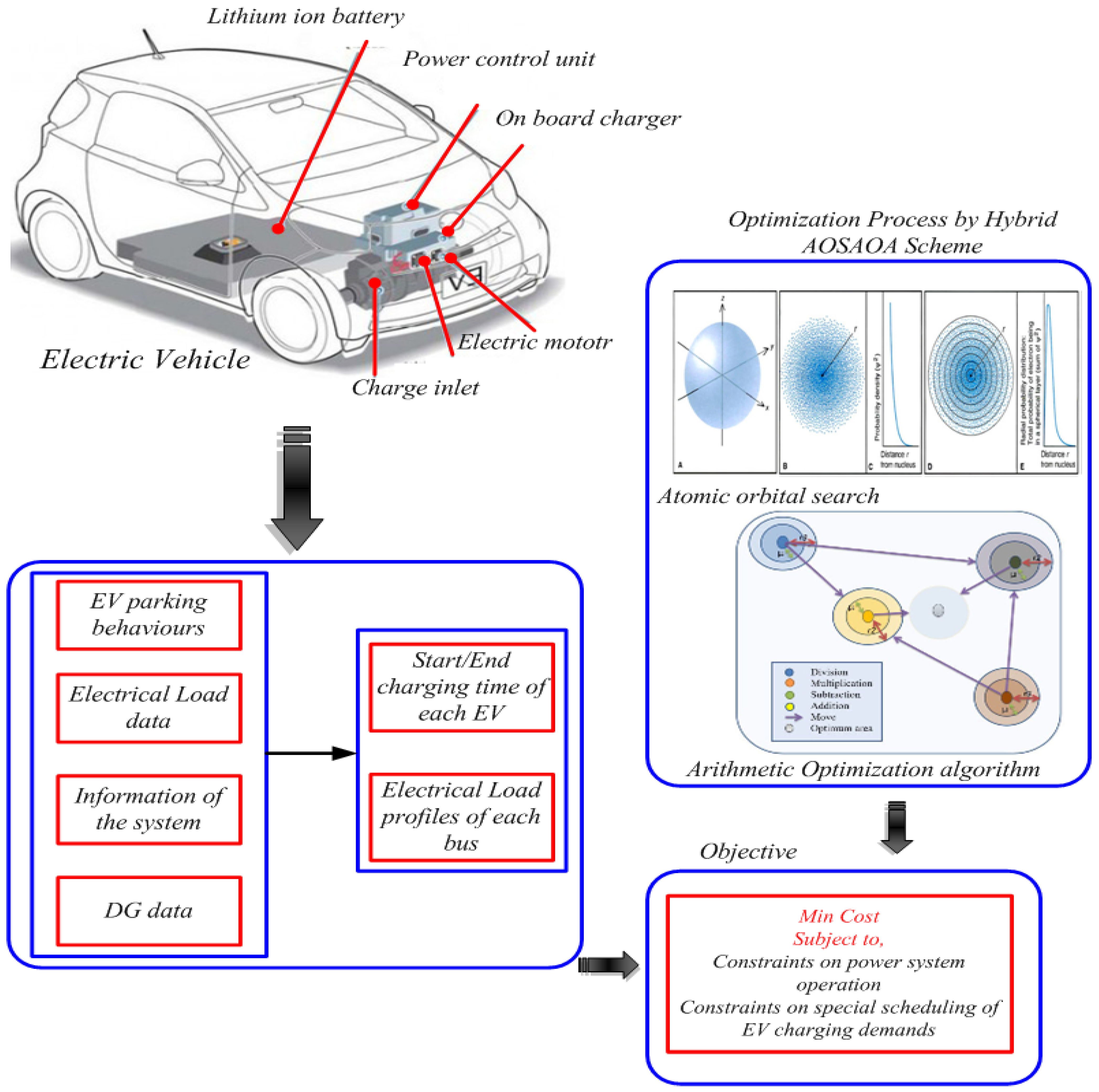
4. Proposed Approach of Atomic Orbital Search and Arithmetic Optimization Algorithm (AOSAOA)

The proposed hybrid scheme will be the joint execution of both the AOS and AOA. AOS depends on certain principles of quantum mechanics and the quantum atomic model under a common configuration of electrons [35]. AOA uses the distribution behavior of major arithmetic operators in mathematics, involving (multiplication, division, subtraction, and addition) [36]. Commonly it is referred to as the AOSAOA technique. The structure of AOA is shown in Figure 2.

4.1. Step by Step Process of AOA

Step 1: Initialization

Determine the initial positions of solution candidates in the search space.

Step 2: Random generation

The initialization procedure generates input parameters randomly using the following Equation (41),

$$X=\left[\begin{array}{cccc}{S}_{11}& S_{12}& \dots & S_{1n}\\ S_{21}& S_{22}& \dots & S_{2n}\\ :& :& :& :\\ S_{n1}& S_{n2}& \dots & S_{nn}\end{array}\right].$$

(41)

Here, X specifies the input parameters of the system.

The minimal objective function is skilled with the optimal process.

Step 3: Fitness Function

Evaluate the fitness values of initial solution candidates as in Equation (42).

$$\mathsf{\Phi }=Min{\displaystyle \sum _{i=1}^n{C}_i}.$$

(42)

Step 4: Determine the binding state, binding energy, and lowest energy level of the atom.

Step 5: For the kth imaginary layer, determine the binding energy and binding state of the layer.

Step 6: Distribute candidates’ solutions in the imaginary layers.

Step 7: Generate a random integer as the number of imaginary layers, which are around the nucleus of an atom.

Step 8: Determine the lowest energy level for the candidate in the kth layer.

Step 9: For the ith candidate solution in the kth layer, generate random updating parameters.

Step 10: Determine the photon rate for the ith candidate solution in the kth layer. Determine the binding state and binding energy of the atom and determine the lowest energy level for the candidate in the atom.

Step 11: Termination

If the number of subjects in the census is equal, check the end method. If not, go to step 4. If the end criteria are not met, go to step 3. If you are satisfied with the finished condition, then find the right solution. Figure 3 display the flow chart of AOA.

4.2. Steps of Arithmetic Optimization Algorithm

Arithmetic is the fundamental component of numerical theory, and it is one of the most important components of modern mathematics, as well as analysis, geometry, and algebra. Arithmetic operators (i.e., subtraction, division, addition, and multiplication) are common calculation methods used to read numbers.

4.3. Step by Step Process of GRFA

Step 1: Initialization phase

In AOA, the process of optimization starts with candidate solutions (X) indicated in Matrix (43). These are randomly generated and the best solution for the candidate for each duplication is considered the most complete or best solution.

$$X=\left[\begin{array}{cccc}{S}_{11}& S_{12}& \dots & S_{1n}\\ S_{21}& S_{22}& \dots & S_{2n}\\ :& :& :& :\\ S_{n1}& S_{n2}& \dots & S_{nn}\end{array}\right]$$

(43)

Here, X Shows the systems input parameters.

Step 2: Fitness Function

Evaluate the fitness values of the initial solution candidates.

Step 3: Exploration phase

In this section, the behavior of AOA is introduced, and Figure 3 show the flowchart of AOA. According to arithmetic staff, mathematical calculators using a multiplication (M) operator or even division (D) obtain higher resolutions or distributed values (see various rules) that bind them to the testing method. Due to their high dispersion, these operators (M and D) are not able to easily approach the target.

Step 4: Exploitation phase

At this stage, the AOA exploitation strategy is introduced. Arithmetic staff and arithmetic calculators using add (A) or subtraction (S) find very dense results referring to the exploitative method. Due to their low dispersion, these operators (A and S) can easily approach the target.

Step 5: Termination

If the number of subjects in the census is equal, check the end method. If not, move to step 4. Go to step 3 if the end criteria are not met. If you satisfy the finish condition, find the right solution.

5. Results and Discussion

A hybrid scheme was proposed based on an optimal location electric vehicles parking lot (PL) and the capacitor’s on-grid profile of voltage and power loss. With this proper control, the perfect placement of the capacitor on the grid and parking lot of EVs on the grid, depletion of reactive and real power loss, and voltage profile are optimally improved. Furthermore, the implementation of the proposed AOSAOA model was developed by the MATLAB/Simulink platform, and the efficiency of the proposed model was likened to other techniques.

The proposed method was tested on 31 buses with 23 kV in a distribution system consisting of 415 V permanent networks (J. Grainger and S. Civanlar) [37]. S. Deilami et al. [38] connected to several low-voltage home loads, and curves in daily loads were completed using a set of high sensitivity options. K. Clement-Nyns et al. [39] proposed integrated charging where the grid load factor is amplified, and power loss is reduced by flexible and quadratic planning techniques. D. Thukaram et al. [40] proposed a method tested to analyze the electrical levels of several distribution networks at a rate of R/X. The application of this method is for reactive power optimum location and planning network reconfiguration.

Figure 4 show PEV charging with different penetrations of no PEV, 16% PEV, and 32% PEV. Here, the no PEV is presented. The no PEV flows from 0.85 p.u at the period of 1 h, and it increases up to 0.87 p.u. at the period of 7 h. The 16% PEV flows from 0.84 p.u at the time period of 1 h, and it increases up to 0.89 p.u. at the time period of 7 h. The 32% PEV flows from 0.83 p.u at the time period of 1 h, and at the time period of 12 h, it increases up to 0.98 p.u, and then it reduces to 0.85 p.u at the time period of 24 h. Figure 5 show the PEV charging with different penetrations of no PEV, 47% PEV, and 63% PEV. Here, in the subplot, the no PEV is presented. The no PEV flows from 0.919 p.u at the time period of 1 h, and it increases up to 0.92 at the time period of 5 h. The 47% PEV flows from 0.918 p.u at the time period of 1 h, and it reduces up to 0.81 at the time period of 5 h. The 63% PEV flows from 0.919 p.u at the time period of 1 h, and at the time period of 12 h, it increases up to 0.95 p.u, and then reduces to 0.91 p.u at the time period of 24 h. Figure 6 show the PEV penetration of the weakest power voltage of no PEV, 16% PEV, and 32% PEV. Here, in subplot (a), the no PEV is presented. The no PEV flows from 0.93 p.u at the time period of 1 h, and at the time period of 12 h, the no PV flows up to 0.97 p.u, and then reduces to 0.95 p.u at the time period of 24 h. The 16% PEV flows from 0.92 p.u at the time period of 1 h, and at the time period of 12 h, it increases up to 0.98 p.u, and then reduces to 0.96 p.u at the time period of 24 h. The 32% PEV flows from 0.94 p.u at the time period of 1 h, and at the time period of 12 h, it increases up to 0.97 p.u, and then reduces to 0.96 p.u at the time period of 24 h. Figure 7 show the PEV penetration of the weakest power voltage of No PEV, 47%% PEV and 63% PEV. Here, in the subplot, the no PEV is presented. The no PEV flows from 0.919 p.u at the time period of 1 h, and it increases up to 0.92 at the time period of 5 h. The 47% PEV flows from 0.918 p.u at the time period of 1 h, and it increases up to 0.937 p.u. at the time period of 5 h. The 63% PEV flows from 0.929 p.u at the time period of 1 h, and at the time period of 12 h, it reduces to 0.918 p.u, and then increases up to 0.948 p.u at the time period of 24 h.

Figure 8 show the PEV penetration of total power loss of no PEV, 16% PEV, and 32% PEV. Here, in the subplot, the no PEV is presented. The no PEV flows from 29 kW at the time period of 1 h, and at the period of 8 h, the no PEV flows up to 6 kW, and then reduces to 3 kW at the time period of 12 h. The 16% PEV flows from 29 kW at the time period of 1 h, and at the period of 8 h, it reduces to 12 kW, and then reduces to 3 kW at the time period of 12 h. The 32% PEV flows from 30 kW at the period of 1 h, and at the time period of 12 h, it reduces to 3 kW, and then increases up to 24 kW at the time period of 24 h. Figure 9 show the PEV penetration of total power loss of no PEV, 47% PEV, and 63% PEV. Here, in the subplot, the no PEV is presented. The no PEV flows from 24 kW at the period of 1 h, and it decreases to 3 kW at the period of 12 h. The 47% PEV flows from 27 kW at the period of 1 h, and it reduces to 4 kW at the time period of 12 h. The 63% PEV flows from 26 kW at the period of 1 h, and at the period of 12 h, it reduces to 8 kW, and then increases up to 20 kW at the period of 24 h.

Figure 10 show the PEV penetration of total power consumption of no PEV, 47% PEV, and 63% PEV. Here, in the subplot, the no PEV is presented. The no PEV flows from 830 kW at the period of 1 h, and it decreases to 300 kW at the time period of 12 h. The 47% PEV flows from 820 kW at the time period of 1 h, and it reduces to 370 kW at the time period of 12 h. The 63% PEV flows from 830 kW at the period of 1 h, and at the time period of 12 h, it reduces to 450 kW, and then increases up to 700 kW at the time period of 24 h. Figure 11 show the PEV penetration of total power consumption of no PEV, 16% PEV, and 32% PEV. Here, in the subplot, the no PEV is presented. The no PEV flows from 820 kW at the time period of 1 h, and it decreases to 280 kW at the time period of 12 h. The 16% PEV flows from 830 kW at the period of 1 h, and it reduces to 340 kW at the period of 12 h. The 32% PEV flows from 840 kW at the time period of 1 h, and at the period of 12 h, it reduces to 290 kW, and then increases up to 730 kW at the time period of 24 h.

Figure 12 show the fixed charge–rate coordination integrating capacitor of no PEV, 16% PEV, and 32% PEV. Here, in the subplot, the no PEV is presented. The no PEV flows from 0.93 p.u at the time period of 1 h, and it increases up to 0.976 p.u at the time period of 12 h. The 16% PEV flows from 0.956 p.u at the time period of 1 h, and it increases up to 0.981 p.u at the time period of 12 h. The 32% PEV flows from 0.95 p.u at the time period of 1 h, and at the time period of 12 h, it increases up to 0.99 p.u, and then reduces to 0.95 p.u at the time period of 24 h. Figure 13 show the fixed charge-rate coordination integrating capacitor of no PEV, 47% PEV, and 63% PEV. Here, in the subplot, the no PEV is presented. The no PEV flows from 0.928 p.u at the period of 1 h, and it increases up to 0.978 p.u at the period of 12 h. The 47% PEV flows from 0.94 p.u at the time period of 1 h, and it increases up to 0.982 p.u at the period of 12 h. The 63% PEV flows from 0.948 p.u at the time period of 1 h, and at the time period of 12 h, it increases up to 0.98 p.u, and then reduces to 0.958 p.u at the time period of 24 h.

Figure 14 show the PEV penetration of total power loss of no PEV, 16% PEV, and 32% PEV. Here, in the subplot, the no PEV is presented. The no PEV flows from 24 kW at the time period of 1 h, and it decreases to 6 kW at the time period of 9 h. The 16% PEV flows from 24 kW at the time period of 1 h, and it reduces to 8 kW at the time period of 9 h. The 32% PEV flows from 25 kW at the time period of 1 h, and at the time period of 12 h, it reduces to 2 kW, and then increases up to 20 kW at the time period of 24 h. Figure 15 show the PEV penetration of total power loss of no PEV, 47% PEV, and 63% PEV. Here, in the subplot, the no PEV is presented. The no PEV flows from 24 kW at the time period of 1 h, and it decreases to 2.5 kW at the time period of 12 h. The 47% PEV flows from 25 kW at the time period of 1 h, and it reduces to 4 kW at the time period of 12 h. The 63% PEV flows from 24 kW at the time period of 1 h, and at the time period of 12 h, it reduces to 10 kW, and then increases up to 20 kW at the time period of 24 h. Figure 16 show the fixed charge—the rate of total power consumption of no PEV, 16% PEV, and 32% PEV. Here, in the subplot, the no PEV is presented. The no PEV flows from 820 kW at the time period of 1 h, and it reduces to 260 kW at the time period of 11 h. The 16% PEV flows from 825 kW at the time period of 1 h, and it reduces to 320 kW at the time period of 11 h. The 32% PEV flows from 830 kW at the time period of 1 h, and at the time period of 12 h, it reduces to 260 kW and then increases up to 780 kW at the time period of 24 h.

Figure 17 show the PEV penetration of total power consumption of no PEV, 47% PEV, and 63% PEV. Here, in the subplot, the no PEV is presented. The no PEV flows from 820 kW at the period of 1 h, and it decreases to 280 kW at the period of 10 h. The 47% PEV flows from 825 kW at the period of 1 h, and it reduces to 300 kW at the period of 10 h. The 63% PEV flows from 830 kW at the period of 1 h, and at the time period of 12 h, it reduces to 260 kW, and then increases up to 780 kW at the period of 24 h.

The proposed analysis with uncoordinated and coordinated levels is shown in Figure 18. Figure 18 show the bar chart proposed method satisfaction level with comparison. When uncoordinated, all customers are satisfied, but the satisfaction level of service is low. When coordination is applied, the PEV customer satisfaction is only three. The success of this approach is to satisfy both the client and the customer, and a limited amount of PEV connection proposed.

Table 1. PEV charging on the distribution system.

Methods	PEV (%)	$\Delta \mathit{V}(\%)$	Increase (%)	Satisfaction Ratio
No PEV Uncoordinated	0	7.35	0	-
	16	7.61	6.97	-
	32	8.95	14.59	-
	47	17.72	33.85	-
	63	19.16	6.96	-
Coordinated	16	7.43	13.67	18/4
	32	7.47	12.32	15/7
	47	8.61	17.53	8/14
	63	9.91	5.53	3/19
Coordinated with capacitor and OLTC switching	16	4.96	5.53	22/0
	32	4.99	11.86	22/0
	47	6.32	17.28	22/0
	63	7.34	23.03	22/0

Note: Table 1 show achieving the satisfaction of PEV customer and utility sides together.

show the PEV charging on the distribution system. When uncoordinated, the car charging process starts immediately but randomly without following system parameters. The distribution system will deal with many problems, such as overload, high power loss, and unacceptable power outages. When coordinated, in order to overcome the harmful effects of un insulated charges of PEV on the distribution system, a real-time method of coordinating 5 min PEV charging is suggested in this paper. Once the car is connected to the charger, the charging process will start only after the central controller decision. The AOSAOA algorithm used optimizes PEV arrivals, and all system barriers are satisfied.

Table 2. Charging power limit and variation limit.

EV	Charging Power Limit	Charging Power Variation Limit
100	500 kW	250 kW
200	1000 kW	750 kW
300	1875 kW	1000 kW

show the charging variation limit and charging power limit. In 100 EV, the charging power variation limit is 250 kW, and the charging power limit is 500 kW. In 200 EV, the charging power limit is 1000 kW and the charging power variation limit is 750 kW. In 300 EV, the charging power limit is 1875 kW, and the charging power variation limit is 1000 kW.

6. Conclusions

In this manuscript, the location determination of an electric vehicles parking lot and capacitors in grid care of voltage profile and power loss by atomic orbital search and arithmetic optimization algorithm optimizer was proposed. The proposed technique performances were analyzed in the MATLAB/Simulink working platform. The performance of the proposed and existing techniques were graphically illustrated. The proposed approach was analyzed under the perfect location of capacitors and parking of electric vehicles on the network. The AOSAOA approach optimized the EVPL’s participation in various energy and ancillary services markets, including the effects of capacity payments. The benefit of EVPL was obtained using the proposed approach and its performance was higher than the existing approach in terms of the analysis of the decrease in the loss of real and reactive power and the change of the voltage profile. By utilizing the proposed hybrid technique, the system provides an optimal solution through the least calculation time. Analysis of total power loss and total power consumption of EVs in PL, the analysis of PV power at different PEVs, and fixed charge-rate were also examined. To analyze the performance of the projected approach, the simulation results were analyzed and compared with methods such as PEV uncoordinated, coordinated, and coordinated with the capacitor.

References

1. Rajabi-Ghahnavieh, A.; Sadeghi-Barzani, P. Optimal Zonal Fast-Charging Station Placement Considering Urban Traffic Circulation. IEEE Trans. Veh. Technol. 2017, 66, 45–56. [Google Scholar] [CrossRef]
2. Zhang, H.; Moura, S.J.; Hu, Z.; Song, Y. PEV Fast-Charging Station Siting and Sizing on Coupled Transportation and Power Networks. IEEE Trans. Smart Grid 2018, 9, 2595–2605. [Google Scholar] [CrossRef]
3. Hosseini, M.; MirHassani, S.A. Refueling-station location problem under uncertainty. Transp. Res. Part E 2015, 84, 101–111. [Google Scholar] [CrossRef]
4. Yildiz, B.; Arslan, O.; Karasan, O.E. A branch and price approach for routing and refueling station location model. Eur. J. Oper. Res. 2016, 248, 815–826. [Google Scholar] [CrossRef] [Green Version]
5. MirHassani, S.A.; Ebrazi, R. A flexible reformulation of the refueling station location problem. Transp. Sci. 2012, 47, 617–628. [Google Scholar] [CrossRef]
6. Wang, G.; Xu, Z.; Wen, F.; Wong, K.P. Traffic-Constrained Multi-objective Planning of Electric Vehicle Charging Stations. IEEE Trans. Power Deliv. 2013, 28, 2363–2372. [Google Scholar] [CrossRef]
7. Yao, W.; Zhao, J.; Wen, F.; Dong, Z.; Xue, Y.; Xu, Y.; Meng, K. A Multi-Objective Collaborative Planning Strategy for Integrated Power Distribution and Electric Vehicle Charging Systems. IEEE Trans. Power Syst. 2014, 29, 1811–1821. [Google Scholar] [CrossRef]
8. Moradi, M.; Abedini, M.; Tousi, S.; Hosseinian, S. Optimal siting and sizing of renewable energy sources and charging stations simultaneously based on Differential Evolution algorithm. Int. J. Electr. Power Energy Syst. 2015, 73, 1015–1102. [Google Scholar] [CrossRef]
9. Amini, M.H.; Moghaddam, M.P.; Karabasoglu, O.J.S.C. Simultaneous allocation of electric vehicles parking lots and distributed renewable resources in smart power distribution networks. Sustain. Cities Soc. 2017, 28, 332–342. [Google Scholar] [CrossRef]
10. Aljanad, A.; Mohamed, A.; Shareef, H.; Khatib, T. A novel method for optimal placement of vehicle-to-grid charging stations in distribution power system using a quantum binary lightning search algorithm. Sustain. Cities Soc. 2018, 38, 174–183. [Google Scholar] [CrossRef]
11. Shaoyun, G.; Liang, F.; Hong, L. Planning of charging stations considering traffic flow and capacity constraints of distribution network. Power Syst. Technol. 2013, 37, 582–589. [Google Scholar]
12. Pazouki, S.; Mohsenzadeh, A.; Ardalan, S.; Haghifam, M. Simultaneous Planning of PEV Charging Stations and DGs Considering Financial, Technical, and Environmental Effects. Can. J. Electr. Comput. Eng. 2015, 38, 238–245. [Google Scholar] [CrossRef]
13. Karmaker, A.K.; Ahmed, M.R.; Hossain, M.A.; Sikder, M.M. Feasibility assessment & design of hybrid renewable energy based electric vehicle charging station in Bangladesh. Sustain. Cities Soc. 2018, 39, 189–202. [Google Scholar]
14. Mozafar, M.R.; Moradi, M.H.; Amini, M.H. A simultaneous approach for optimal allocation of renewable energy sources and electric vehicle charging stations in smart grids based on improved GAPSO algorithm. Sustain. Cities Soc. 2017, 32, 627–637. [Google Scholar] [CrossRef]
15. Atwa, Y.M.; El-Saadany, E.F.; Salama, M.M.A.; Seethapathy, R. Optimal Renewable Resources Mix for Distribution System Energy Loss Minimization. IEEE Trans. Power Syst. 2010, 25, 360–370. [Google Scholar] [CrossRef]
16. Teng, J.; Luan, S.; Lee, D.; Huang, Y. Optimal Charging/Discharging Scheduling of Battery Storage Systems for Distribution Systems Interconnected With Sizeable PV Generation Systems. IEEE Trans. Power Syst. 2013, 28, 1425–1433. [Google Scholar] [CrossRef]
17. Mazidi, M.; Zakariazadeh, A.; Jadid, S.; Siano, P. Integrated scheduling of renewable generation and demand response programs in a microgrid. Energy Convers. Manag. 2014, 86, 1118–1127. [Google Scholar] [CrossRef]
18. GeunKim, J.; Kuby, M. The deviation-flow refueling location model for optimizing a network of refueling stations. Int. J. Hydrogen Energy 2012, 28, 5406–5420. [Google Scholar]
19. Hung, D.Q.; Mithulananthan, N.; Lee, K.Y. Determining PV Penetration for DistributionSystems With Time-Varying Load Models. IEEE Trans. Power Syst. 2014, 29, 3048–3057. [Google Scholar] [CrossRef]
20. Yu, H.; Chung, C.Y.; Wong, K.P.; Lee, H.W.; Zhang, J.H. Probabilistic Load Flow Evaluation With Hybrid Latin Hypercube Sampling and Cholesky Decomposition. IEEE Trans. Power Syst. 2009, 24, 661–667. [Google Scholar] [CrossRef]
21. Sachan, S.; Amini, M. Optimal allocation of EV charging spots along with capacitors in smart distribution network for congestion management. Int. Trans. Electr. Energy Syst. 2020, 30, e12507. [Google Scholar] [CrossRef]
22. Aggarwal, S.; Singh, A. Impact analysis of electric vehicle charging station integration with distributed generators on power systems. Int. J. Circuit Theory Appl. 2021, 49, 1811–1827. [Google Scholar] [CrossRef]
23. Bilal, M.; Rizwan, M. Integration of electric vehicle charging stations and capacitors in distribution systems with vehicle-to-grid facility. Energy Sources Part A Recovery Util. Environ. Eff. 2021, 41, 1828–1837. [Google Scholar] [CrossRef]
24. Ahmadi, M.; Hosseini, S.; Farsadi, M. Optimal Allocation of Electric Vehicles Parking Lots and Optimal Charging and Discharging Scheduling using Hybrid Metaheuristic Algorithms. J. Electr. Eng. Technol. 2021, 16, 759–770. [Google Scholar] [CrossRef]
25. Chen, L.; Xu, C.; Song, H.; Jermsittiparsert, K. Optimal sizing and sitting of EVCS in the distribution system using metaheuristics: A case study. Energy Rep. 2021, 7, 208–217. [Google Scholar] [CrossRef]
26. Raja, C.S.; Kumar, V.N.M.; Senthil, K.J.; Nesamalar, J.J. Enhancing system reliability by optimally integrating PHEV charging station and renewable distributed generators: A Bi-Level programming approach. Energy 2021, 229, 120746. [Google Scholar] [CrossRef]
27. Rajesh, P.; Shajin, F. Optimal allocation of EV charging spots and capacitors in distribution network improving voltage and power loss by Quantum-Behaved and Gaussian Mutational Dragonfly Algorithm (QGDA). Electr. Power Syst. Res. 2021, 194, 107049. [Google Scholar] [CrossRef]
28. Luo, L.; Wei, G.; Suyang, Z.; He, H.; Song, G.; Jun, H.; Zhi, W.; Xiaobo, D. Optimal planning of electric vehicle charging stations comprising multi-types of charging facilities. Appl. Energy 2018, 226, 1087–1099. [Google Scholar] [CrossRef]
29. Andrenacci, N.; Ragona, R.; Valenti, G. A demand-side approach to the optimal deployment of electric vehicle charging stations in metropolitan areas. Appl. Energy 2016, 182, 39–46. [Google Scholar] [CrossRef]
30. Zheng, Y.; Song, Y.; Hill, D.; Meng, K. Online Distributed MPC-Based Optimal Scheduling for EV Charging Stations in Distribution Systems. IEEE Trans. Ind. Inform. 2019, 15, 638–649. [Google Scholar] [CrossRef]
31. Song, Y.; Zheng, Y.; Hill, D. Optimal Scheduling for EV Charging Stations in Distribution Networks: A Convexified Model. IEEE Trans. Power Syst. 2016, 32, 1574–1575. [Google Scholar] [CrossRef]
32. Fazeli, S.; Venkatachalam, S.; Chinnam, R.; Murat, A. Two-Stage Stochastic Choice Modeling Approach for Electric Vehicle Charging Station Network Design in Urban Communities. IEEE Trans. Intell. Transp. Syst. 2020, 22, 3038–3053. [Google Scholar] [CrossRef] [Green Version]
33. Zhang, H.; Tang, L.; Yang, C.; Lan, S. Locating electric vehicle charging stations with service capacity using the improved whale optimization algorithm. Adv. Eng. Inform. 2019, 41, 100901. [Google Scholar] [CrossRef]
34. Gong, L.; Cao, W.; Liu, K.; Zhao, J. Optimal Charging Strategy for Electric Vehicles in Residential Charging Station under Dynamic Spike Pricing Policy. Sustain. Cities Soc. 2020, 63, 102474. [Google Scholar] [CrossRef]
35. Azizi, M. Atomic orbital search: A novel metaheuristic algorithm. Appl. Math. Model. 2021, 93, 657–683. [Google Scholar] [CrossRef]
36. Abualigah, L.; Diabat, A.; Mirjalili, S.; AbdElaziz, M.; Gandomi, A. The Arithmetic Optimization Algorithm. Comput. Methods Appl. Mech. Eng. 2021, 376, 113609. [Google Scholar] [CrossRef]
37. Grainger, J.; Civanlar, S. Volt/Var Control on Distribution Systems with Lateral Branches Using Shunt Capacitors and Voltage Regulators Part I: The Overall Problem. IEEE Trans. Power Appar. Syst. 1985, 104, 3278–3283. [Google Scholar] [CrossRef]
38. Deilami, S.; Masoum, A.; Moses, P.; Masoum, M. Real-Time Coordination of Plug-In Electric Vehicle Charging in Smart Grids to Minimize Power Losses and Improve Voltage Profile. IEEE Trans. Smart Grid 2011, 2, 456–467. [Google Scholar] [CrossRef]
39. Clement-Nyns, K.; Haesen, E.; Driesen, J. The Impact of Charging Plug-In Hybrid Electric Vehicles on a Residential Distribution Grid. IEEE Trans. Power Syst. 2010, 25, 371–380. [Google Scholar] [CrossRef] [Green Version]
40. Thukaram, D.; Banda, H.W.; Jerome, J. A robust three phase power flow algorithm for radial distribution systems. Electr. Power Syst. Res. 1999, 50, 227–236. [Google Scholar] [CrossRef]
Figure 1. Overview of electric vehicle parking lot based on the proposed approach.
Energies 15 04202 g001
Figure 2. Structure of AOA.
Energies 15 04202 g002
Figure 3. Flowchart of AOA.
Energies 15 04202 g003
Figure 4. PEV charging with diverse penetration of no PEV, 16% PEV, and 32% PEV.
Energies 15 04202 g004
Figure 5. PEV charging with different penetration of no PEV, 47% PEV, and 63% PEV.
Energies 15 04202 g005
Figure 6. PEV penetration of weakest power voltage no PEV, 16% PEV, and 32% PEV.
Energies 15 04202 g006
Figure 7. PEV penetration of weakest power voltage of no PEV, 47% PEV, and 63% PEV.
Energies 15 04202 g007
Figure 8. PEV penetration of total power loss of no PEV, 16% PEV, and 32% PEV.
Energies 15 04202 g008
Figure 9. PEV penetration of total power loss no PEV, 47% PEV, and 63% PEV.
Energies 15 04202 g009
Figure 10. PEV penetration of total power consumption no PEV, 47% PEV, and 63% PEV.
Energies 15 04202 g010
Figure 11. PEV penetration of total power consumption no PEV, 16% PEV, and 32% PEV.
Energies 15 04202 g011
Figure 12. Fixed-charge–rate coordination integrating capacitor no PEV, 16% PEV, and 32% PEV.
Energies 15 04202 g012
Figure 13. Fixed charge-rate coordination integrating capacitor no PEV, 47% PEV, and 63% PEV.
Energies 15 04202 g013
Figure 14. Fixed charge–rate of total power loss of no PEV, 16% PEV, and 32% PEV.
Energies 15 04202 g014
Figure 15. Fixed charge–rate of total power loss of no PEV, 47% PEV, and 63% PEV.
Energies 15 04202 g015
Figure 16. Fixed charge–rate of total power consumptionof no PEV, 16% PEV, and 32% PEV.
Energies 15 04202 g016
Figure 17. Fixed charge–rate of total power consumption of no PEV, 47% PEV, and 63% PEV.
Energies 15 04202 g017
Figure 18. Analysis of proposed with uncoordinated and coordinated level.
Energies 15 04202 g018