The Online Parameter Identification Method of Permanent Magnet Synchronous Machine under Low-Speed Region Considering the Inverter Nonlinearity

Abstract

To realize the high-performance control of a servo system, parameter accuracy is very important for the design of the controller. Thus, the online parameter identification method has been widely researched. However, the nonlinearity of the inverter will lead to an increase in resistance identification error and the fluctuation of inductance identification results. Especially in the low-speed region, the influence of the inverter is more obvious. In this paper, an offline neural network is proposed considering the parasitic capacitance to identify the nonlinearity of the inverter. Based on the Kirchhoff equation in the static state of the motor, the nonlinear voltage equation is established, and the gradient direction of the weight coefficients has been re-derived. Using the gradient descent method, the identification error can converge to zero. Moreover, the d-axis voltage equation is established considering the nonlinearity of the inverter and an online adaptive observer was proposed. Based on the Lyapunov equation, the adaptive laws are derived. Further, the decoupling of the deadtime voltage and resistance voltage is realized by using the result of neural network identification. With the proposed algorithm, nonlinear identification of the inverter characteristics is realized, and the resistance and inductance identification accuracy in the low-speed region is improved. The effectiveness of the proposed methods is verified through experimental results.

1. Introduction

1.1. Motivation

To get high dynamic control performance, the current controller in a servo system is highly dependent on the accuracy of the permanent magnet synchronous machine parameters [1]. Thus, the online parameter identification algorithm is researched to get the resistance and inductance in real-time. However, due to the lack of a voltage sensor, the identification algorithm can only use the output signal of the current controller as the actual voltage signal [2]. However, there is an inevitable error between the voltage reference and the actual voltage signal caused by the deadtime effect. The deadtime effect is caused by the deadtime inserted by the digital controller to prevent the switch on the same bridge arm from being turned on at the same time, which will result in a short circuit fault. However, this inserted constant time gap will lead to a voltage disturbance in the system and cause a fifth and seventh harmonic phase currents [3]. These current harmonics will identify the fluctuation inductance value. In addition, the deadtime effect will cause errors between the given reference voltage and the actual output voltage, leading to the coupling between the deadtime voltage and resistance voltage drop [4] and causing the identification error of the resistance parameter.

1.2. Problem Statement

Considering the parasitic capacitance, the relationship between the deadtime effect voltage and load current is nonlinear. Therefore, it is hard to realize the identification of deadtime characteristics without linear equivalence at different current amplitudes, and the linear equivalence will cause large identification errors at low current conditions. Moreover, because of the voltage coupling of the deadtime voltage and resistance voltage drop, the resistance and deadtime characteristics cannot be identified online at the same time. Thus, to achieve accurate online identification of the resistance and inductance parameters in the low-speed region, it is particularly important to compensate for the deadtime effect.

1.3. Previous Solutions

The existing identification methods for the deadtime effect can be divided into online compensation and offline compensation strategies. Offline compensation methods analyze the characteristics of the deadtime voltage model and establish a mathematical model [5]. Then, the average voltage loss within a switching cycle is calculated and compensated through feedforward. The method of online compensation is mainly to indirectly realize the compensation of the deadtime effect by suppressing the current harmonics introduced by the deadtime [6].

In [7], an offline deadtime compensation method is given, and it concludes that the deadtime compensation voltage is related to the current polarity. To compensate the deadtime effect, the polarity of the current is needed. Due to the limitation of sampling accuracy, the current signal cannot be accurately sampled when the current crosses zero, resulting in compensation errors and additional harmonics. To solve the zero-crossing problem, Ref. [8] utilized the power factor angle to measure the direction of current indirectly and reduce the zero-crossing current sampling error. In [9], the voltage vector of the space vector pulse width modulation (SVPWM) was used to get the zero-crossing position of the phase current. From [9], the three-phase current was divided into six regions, and the compensation behavior was performed only for the phase whose current direction was different from that of other phase currents. From [10], the current angle between i_α and i_β is used to judge the current direction. In addition, Ref. [11] analyzes the influence of the current ripple on the deadtime effect and proposes a current reconstruction method to reduce the disturbance’s interference with model-based compensation. In [12], the deadtime compensation voltage model under the dq-axis was deduced by the flux increment equation, and the relationship between the deadtime voltage and phase current was established. In addition, zero-crossing detection was not required, which made the established model have a better compensation effect under light loads. In [13], the activation time of the voltage vector is reallocated, and the time allocation algorithm is simplified by using the zero vector. The authors of [14] deduce the voltage space vector by introducing maximum, minimum and medium reference voltages and using medium voltage-current polarity to identify the inverter deadtime. In [15], the switching delays are considered, and a novel compensation model is proposed. However, the current polarity is needed for judging the compensation condition, and the parasitic capacitance is not analyzed. From [16], the pulse-based deadtime compensation is researched instead of using current polarity. However, the compensation model is established based on the linear approximation, and the compensation performance will deteriorate under low load conditions. From [7,8,9,10,11,12,13,14,15,16], the current polarity problems are mainly researched. However, the influence of parasitic capacitance is not considered, which will lead to a compensation error under light load conditions. To simulate the nonlinear characteristics, Ref. [17] proposed a linear equivalent model. Setting a current threshold, the compensation voltage is divided into the linear and saturated regions. However, the value of the threshold will affect the compensation performance, and no effective method is given to determine its value. In addition, Refs. [18,19] analyzes the influence of parasitic capacitance on the deadtime effect and finds that the parasitic capacitance has the compensation effect for the deadtime influence. In addition, as the charging and discharging time of the capacitor is related to the load current, the impact of parasitic capacitance is more obvious when the load current is smaller. In [20], the value of parasitic capacitance is changed by applying additional capacitance, and the compensation effect of parasitic capacitance on the deadtime effect is researched. The deadtime effect is directly compensated by setting an appropriate parasitic capacitance. However, this method is cumbersome to operate, and it is difficult to measure the parasitic capacitance and select the appropriate compensation capacitance in a non-laboratory environment. Since it is difficult to obtain accurate parasitic capacitance parameters, the deadtime model of light load for offline identification is hard to establish. The authors of [21] give an auto measurement method to derive the nonlinear characteristics of the inverter output voltage delay curve; the resistance value is needed to calculate the voltage error. However, the resistance is changed along with the temperature, which will lead to identification error.

Because the deadtime effect will produce 5th, 7th, 13th, and 15th harmonics in the phase current, the online compensation of the deadtime can be realized by designing various feedback algorithms to suppress the harmonic current. The authors of [22] present a deadtime online identification algorithm based on the harmonic separation method. Using a low-pass filter to extract the harmonic signal of current. Then, the cascade PI controller is used, which makes the filtered harmonic signal converge to zero. However, the harmonic suppression performance of this method will decrease with the increase in the current frequency, and the parameters of the low pass filter and PI controller need to be selected according to the specific working conditions, which makes the universality of the system reduced. Considering the parasitic capacitance, the relationship between the deadtime effect and current is nonlinear. Therefore, in [23,24], the neural network is used to identify the deadtime effect due to its excellent fitting characteristics of nonlinear functions, and an appropriate adaptive law is designed. The authors of [25] researched the phase of q-axis deadtime compensation voltage and compensation time. In [25], the disturbance voltage of the q-axis is estimated through the disturbance observer, and the compensation time is calculated online. The phase of the compensation voltage is determined adaptively according to the compensation time. However, the effect of parasitic capacitance on the q-axis deadtime voltage is not considered, which will lead to compensation errors under low load conditions. Because the deadtime effect will produce six harmonics in the rotating coordinate system, Ref. [26] use the voltage harmonic in the output of the current PI controller to compensate for the deadtime effect, this method does not use an extra hardware circuit and is easy to implement. However, considering the limitation of bandwidth, the compensation effect will deteriorate in the high-speed region. Moreover, the online deadtime compensation is based on the motor current loop equation, so the resistance parameters need to be used for iterative calculation, which will cause the resistance and deadtime effect to not be able to be identified at the same time. To improve the harmonic suppression performance of the system at high frequencies, an adaptive notch filter is used in [27] to suppress specific harmonics. However, the calculation process of the adaptive notch filter will greatly increase the operation time of the system, and the system delay has a great influence on the suppression performance of the notch filter. In [28], the influence of different modulation methods on the deadtime effect is analyzed, and the nonlinear characteristics are identified by comparing the continuous pulse width modulation (PWM) and discontinuous PWM. However, in practical applications, to ensure the stability of the working conditions, the modulation method cannot usually be changed, so this method is not practical. In [29], a second current harmonic is injected into the DC bus to eliminate the influence of deadtime, but the injected current harmonics will introduce additional torque harmonics into the system.

1.4. Main Contributions

An equivalent nonlinear inverter model considering the parasitic capacitance is established. The neural network model corresponding to the equivalent circuit is established to accurately identify the deadtime effect under any load conditions without using the linear equivalent method. In addition, the identification algorithm of resistance and inductance parameters is optimized, and the parameter identification can be realized at zero and a low speed by using a 1% rated current injection. It greatly reduces the impact on the operation state of the system. The high-performance control of the motor current without parameter setting is realized through the proposed deadtime compensation method and parameter identification algorithm.

1.5. Paper Structure

In this paper, the equivalent nonlinear model of the motor and inverter is first established, then it is transformed into the neural network model. After that, the update algorithm of the weight function is derived. A sinusoidal current with a specified frequency is injected into the d-axis, and the data of phase A current and d-axis voltage are collected. These data are input into the neural network to identify the deadtime model. In addition, an online parameter identification strategy based on the adaptive algorithm is theoretically derived.

The structure of this paper is organized as follows. In the Section 2, the effect of parasitic capacitance on the deadtime model is analyzed. An offline neural network model is established in the Section 3. In the Section 4, the online parameter identification algorithm is deduced. In addition, the corresponding algorithm is verified experimentally in Section 5. Finally, the discussion and conclusion are given in Section 6 and Section 7.

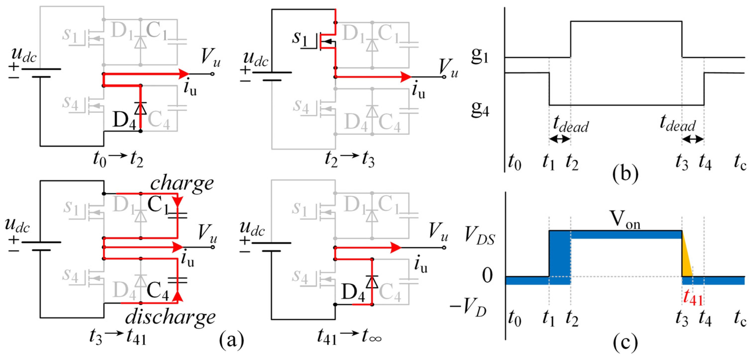
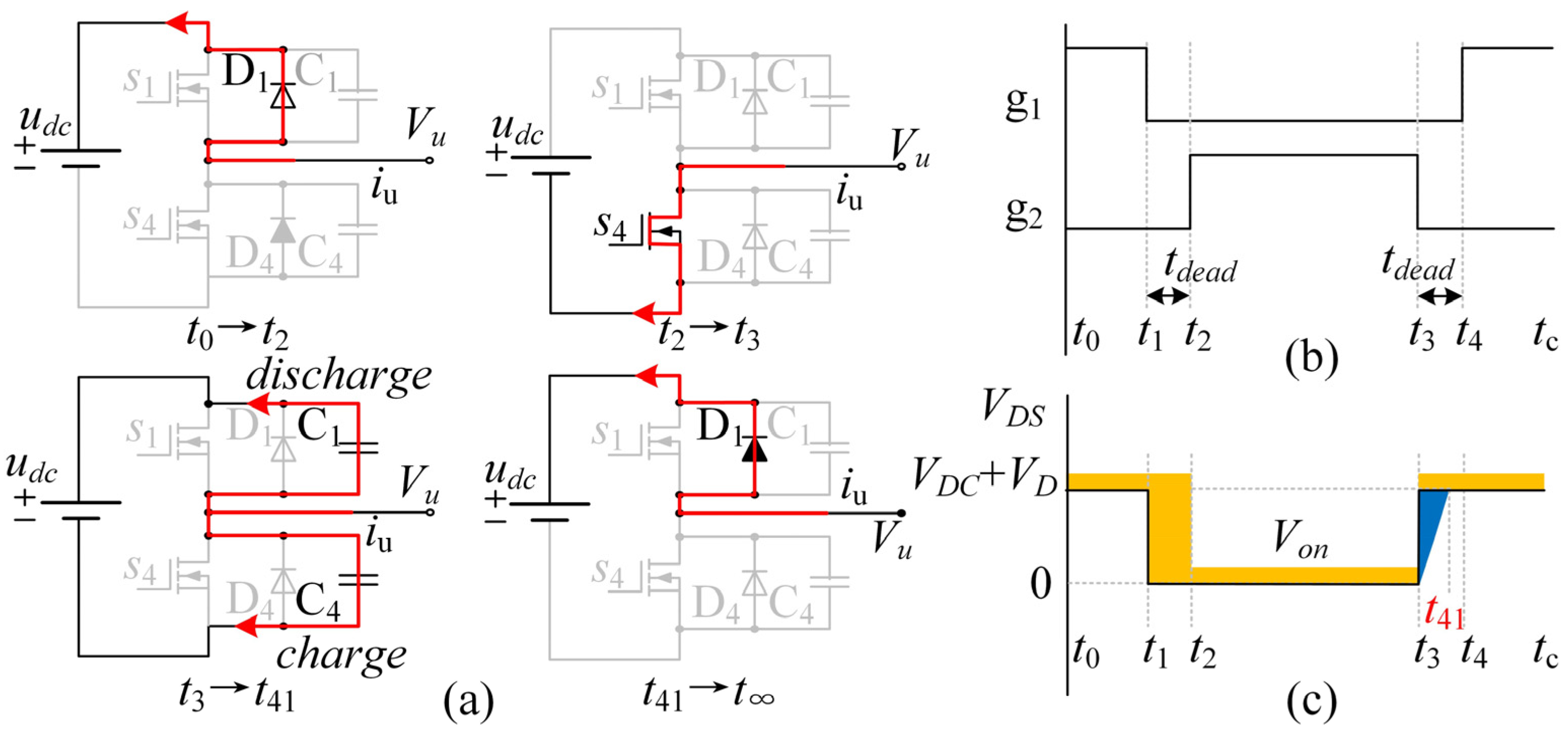
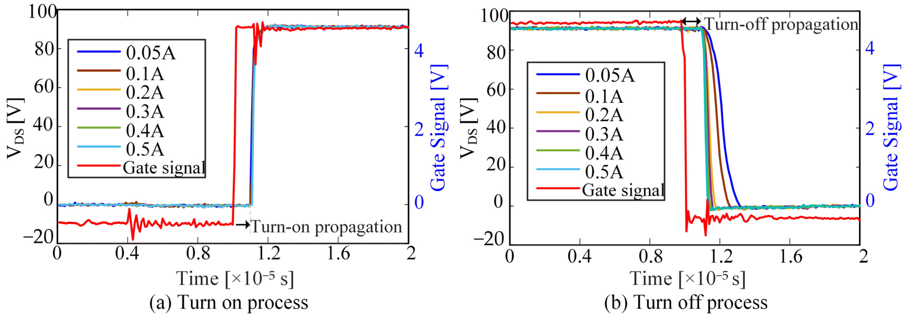
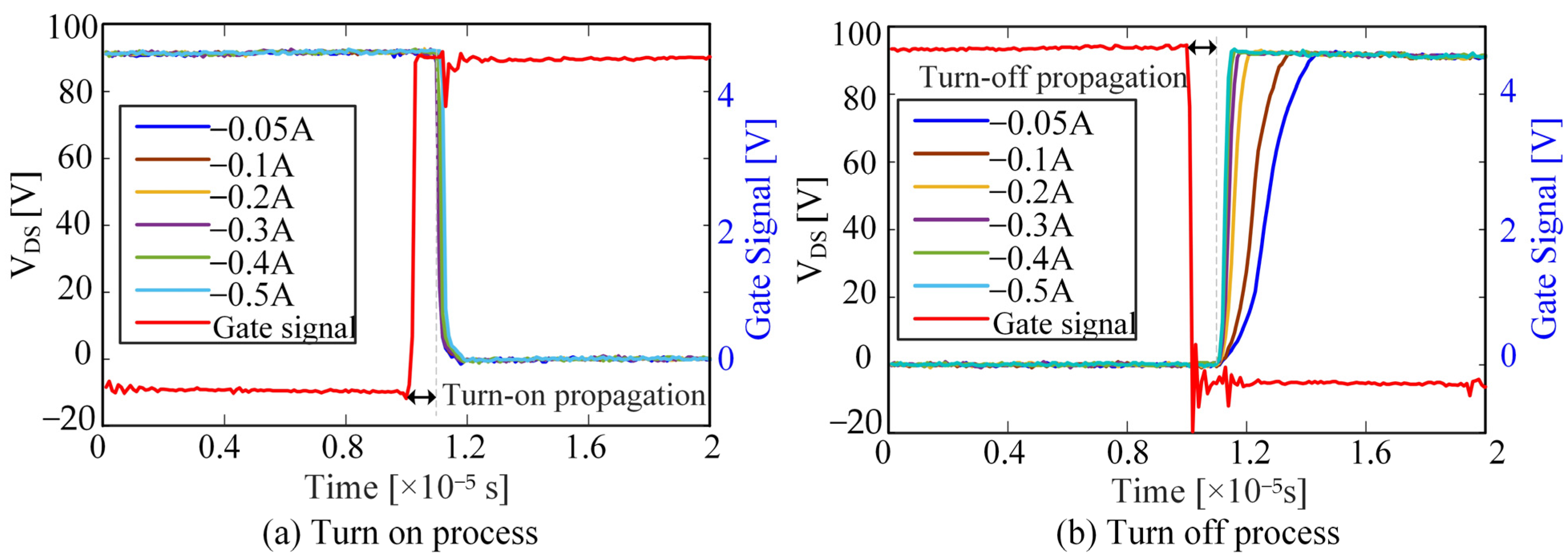
2. The Nonlinearity of Deadtime Effect

Due to the deadtime effect of the inverter, there is an error between the given voltage and the output voltage, and this voltage error will be coupled with the resistance voltage drop, which will result in the identification error of the resistance. Moreover, the voltage disturbance of the deadtime effect will also produce fifth and seventh harmonics in the phase current, resulting in fluctuations in the identification of the inductance parameters. However, considering the influence of parasitic capacitance, the deadtime effect will be affected by the amplitude of the load current and show nonlinear characteristics. The influence of parasitic capacitance on the deadtime effect is analyzed in Figure 1 and Figure 2.

Figure 1 gives the variation process of voltage between the drain and source electrodes in a switching cycle under positive current. In this figure, u_dc is the bus voltage; s₁ and s₄ are the power switches and g₁ are g₂ are the corresponding gate signals; D₁ and D₄ are the freewheeling diodes; C₁ and C₄ are the parasitic capacitances; i_u is the load current; V_u is the output voltage, V_D is the voltage drop of D₁ and D₄, V_DS is the voltage drop of the switch; t_dead stands for the setting dead time; t_c is the setting control period. Figure 1a gives the current trajectory at different switch states. Figure 1b gives the gate signal considering the deadtime, and Figure 1c gives the corresponding output voltage. In this figure, the blue block stands for the voltage drop compared with the ideal voltage and the yellow parts means the voltage is increasing.

During t₀–t₂, according to the gate signal shown in Figure 1b, s₁ is closed and s₄ keeps conducting. The positive load current can only flow through D₄. In this situation, V_u = −V_D. g₂ is turned off at t₁, and g₁ will be turned on at t₂ because of the inserting deadtime. Thus, a voltage loss will be caused during t₁–t₂, which is shown in Figure 1c. At t₂, the gate signal g₁ changes to a high level and s₁ is turned on. At this time, the current loop is changed to s₁ and V_u = u_dc − V_DS. At t₃, g₁ is closed. However, the current will not immediately change to D₄, but will first charge and discharge the parasitic capacitors C₁ and C₄. During this process, the output voltage V_u decreases according to the charging and discharging characteristics of the capacitor. Therefore, the slow change of voltage causes the rise of average voltage during one period, which is shown as the yellow part in Figure 1c. When the capacitor charge and discharge are completed, the current path changes to D₄.

The deadtime effect considering the parasitic capacitance under negative current is shown in Figure 2. The path analysis of current under different switching states is similar to the positive load current. However, the diode voltage drop, switching conduction voltage drop and the deadtime will increase the average voltage. The charging and discharging process of the capacitor will cause a decrease in the average voltage.

Summarizing the deadtime effect model considering parasitic capacitance, the following conclusions can be derived:

(1) In the case of positive current, the switch, diode voltage drop and deadtime cause the average voltage to decrease, while the parasitic capacitance effect increases the average voltage, so the parasitic capacitance has the compensation effect on the deadtime effect.

(2) In the case of negative current, the switch, diode voltage drop and deadtime cause the average voltage to increase, while the parasitic capacitance effect decreases the average voltage. Therefore, the parasitic capacitance also shows the opposite effect of the deadtime effect.

(3) The charging and discharging time of parasitic capacitors are related to the load current. The smaller the load current is, the more obvious the compensation effect of the deadtime effect is.

Therefore, due to the influence of parasitic capacitance, the deadtime effect is not only related to the polarity of the current but also related to the amplitude of the current, which leads to the nonlinear characteristics of the deadtime effect. The deadtime characteristics remain unchanged when the hardware setting is completed. Therefore, an offline neural network is proposed to identify the nonlinear deadtime characteristics.

3. Offline Deadtime Compensation

3.1. Equivalent Identification Model of Deadtime Effect

The identification of the deadtime effect can be built as follows:

In Figure 3, $V_{an}^{*},V_{bn}^{*},V_{cn}^{*}$ stands for the voltage reference of phases A, B and C; D(i_as), D(i_bs) and D(i_cs) are the voltage errors caused by the deadtime effect; R_s and L_s are the phases resistant and inductance; V_a, V_b and V_c are the back electromotive force. To avoid the influence of back EMF on system identification, the motor is kept stationary during the test process, and phase A is coincident with the d-axis. Therefore, Figure 3a can be equivalent to Figure 3b. In Figure 3b, since phase A of the motor stays coincident with d-axis, the voltage of phase A is equal to u_d. When the three-phase load is assumed to be completely symmetrical, the voltage of phases B and C is equal to −0.5 times the voltage of phase A. Therefore, it can be calculated that the line voltage of phases A and B is equal to 1.5 times the d-axis voltage. According to the above calculation, the Kirchhoff voltage equation in Figure 3b can be obtained as follows:

$$-\frac{3}{2}{u}_d+\mathrm{D}(i_{as})+R_s{i}_{as}-R_s{i}_{bs}-\mathrm{D}(i_{bs})=0$$

(1)

According to the current relationship, i_as = −0.5i_bs can be obtained. Substitute it into the above formula to obtain:

$$\mathrm{D}(i_{as})+\mathrm{D}(0.5i_{as})=\raisebox{1ex}{$3$}\!\left/ \!\raisebox{-1ex}{$2$}\right.(u_d^{*}-R_s{i}_{as})$$

(2)

Because D(i_as) is nonlinear, $\mathrm{D}(i_{as})\ne \mathrm{D}(0.5i_{as})$. Therefore, to identify the nonlinear function D(i_as), a three-layer fully connected back propagation neural network is used to identify the function.

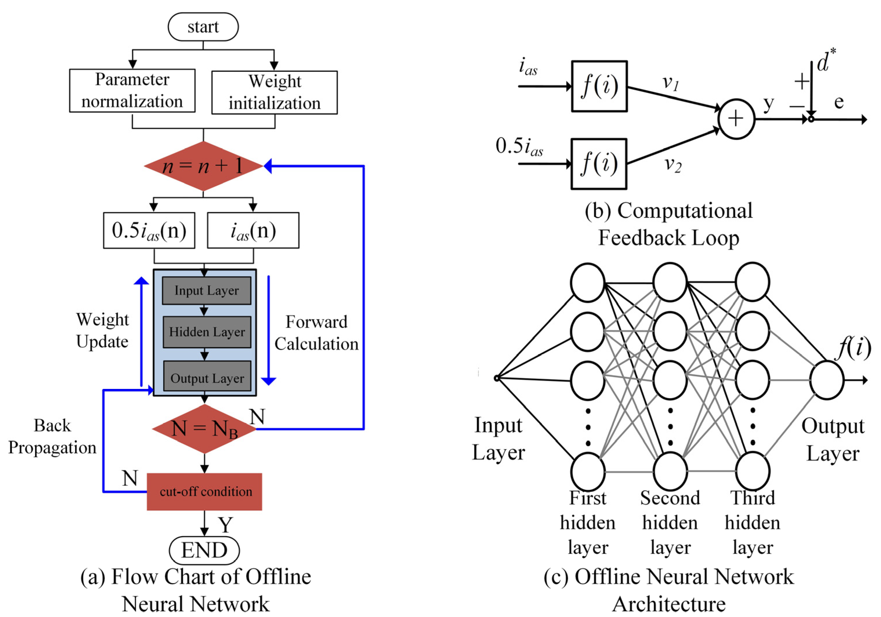
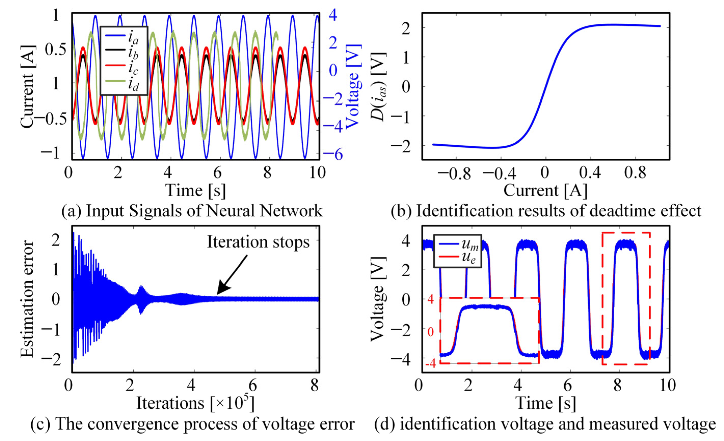
3.2. The Establishment of Neural Network

The neural network identification process is established according to Equation (2), and the principle is shown in Figure 4. Figure 4b gives the identification calculation loop, which is designed through Equation (2). In this figure, f(i) represents the deadtime model to be identified, v₁ is the output of input i_as and v₂ is the output of 0.5i_as and d* represents the ideal voltage, which is defined as $d^{*}=1.5(u_d^{*}-R_s{i}_{as})$. The deadtime identification model is established according to (2), which consists of two inputs, namely i_as and 0.5i_as. In this paper, a three-layer neural network structure is shown in Figure 4c. It is used to identify the deadtime function f(i), and the two inputs at the same time are substituted into the network to calculate the error e. Then, the weight coefficient in the network is updated through the error. The specific process is shown in Figure 4a, in which N_B represents the set batch size, and N represents the number of cycles. According to Figure 4a, the identification process of the neural network is as follows:

First, the measured current and voltage parameters need to be normalized to (0,1) to prevent saturation in the calculation of the network activation function; secondly, the weight value of the established network is initialized. In this study, the weight is randomly selected between 0 and 1 to prevent the network from falling into local optimization due to the ill condition of the initial weight; finally, the current is input into the neural network for forward calculation, and a set of output values can be obtained. After calculating the error, the weight of the neural network is updated through reverse error transmission.

To deduce the forward calculation and weight update process, the calculation flow chart of v₁ is given in Figure 5. The calculation flow of v₂ is similar to v₁. In Figure 5, taking the first hidden layer as an example, the weight coefficient $w_{i_p{j}_L}$ means the weight coefficient connected between the p-th neuron in layer I and the L-th neuron in layer J. $y_{i_p}$ represents the input parameters of the p-th neuron in layer I, $v_{j_L}$ stands for the input of the activation function of the L-th neuron in layer J, φ() is the activation function and the sigmoid function is used in this study, which is expressed as follows:

$$\phi (x)=\frac{2}{1+e^{-ax}}-1$$

(3)

In this study, the back-propagation neural network is used, and its calculation process can be divided into two parts, one is the forward calculation process and the other is the weight reverse update process. These two processes are deduced as follows:

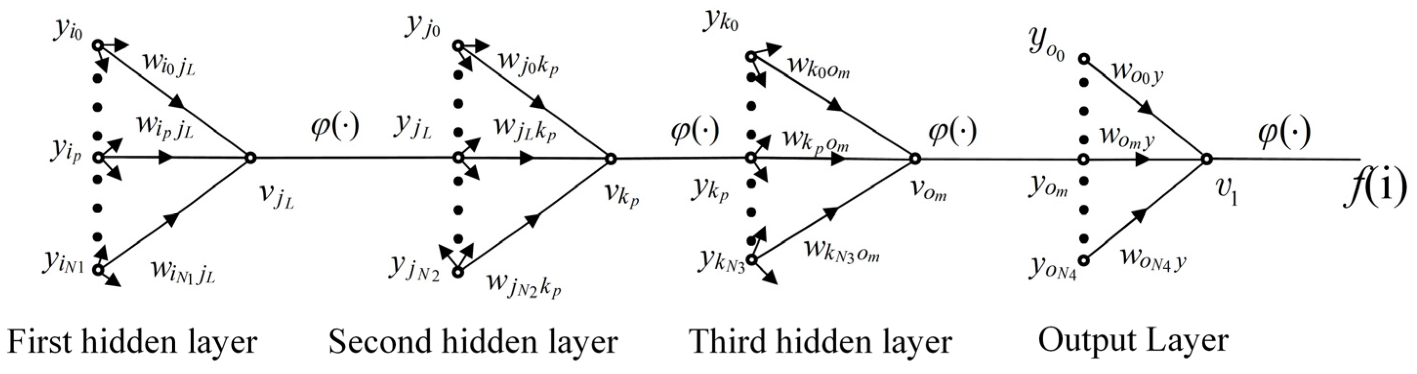
3.2.1. Forward Calculation Process

As shown in Figure 5, to identify the deadtime effect, a three-layer neural network is used to identify the nonlinear function f(i). Taking the output v₁ as an example, it meets the following equation in the forward calculation process:

$$\begin{array}{l}{v}_1={\displaystyle \sum _{m=0}^{N_4}{y}_{o_m}{w}_{o_{m}y}}\\ f(i)=\phi (v_1)\end{array}$$

(4)

In Equation (4), $y_{o_m}$ represents the m-th output of the output layer, $w_{o_m{y}_1}$ represents the weight coefficient from the m-th neuron of the output layer to the output and N₄ represents the number of network neurons of the output layer. The forward calculation process of other layers is similar to Equation (4), and the output layer can be derived as:

$$\begin{array}{l}{v}_1=f(i)\\ v_2=f(i_{as}/2)\\ e(n)=d^{*}-v_1-v_2\end{array}$$

(5)

The error corresponding to the n-th input can be obtained through Equation (5). To prevent the gradient from entering the local optimum during updating, the weight coefficient is updated by batch gradient descent in this study. Therefore, the system error is defined as follows:

$$E(k)=\frac{1}{2}{\displaystyle \sum _{n=1}^{N_B}{e}^2(n)}$$

(6)

In Equation (6), k stands for the iteration period.

3.2.2. Back Propagation Process

After calculating the error according to the forward process, the weight coefficient in the forward path needs to be adjusted according to the error, and the updating process of the weight coefficient is from back to front, so it is called the back propagation process. Because the same neural network is used to identify the function, the weight coefficients of the same layer are the same for two inputs, but output y is different. In addition, according to Equation (6), the batch error is a convex function, so the weight coefficient can be updated by the steepest gradient descent method:

$$W_{I_i{j}_k}=W_{I_{i}j}{}_{{}_k}-\mu {\displaystyle \sum _{n=1}^{N_B}G(n)}/N_B$$

(7)

In Equation (6), G(n) represents the gradient at time interval n. To obtain the gradient of neurons at different layers, the process is divided into two cases:

• For the output layer

From Figure 5, it can be obtained that:

$$\begin{array}{l}{v}_1={\displaystyle \sum _{p=1}^{N_4}{y}_{1o_m}{w}_{o_{m}y}}\\ v_2={\displaystyle \sum _{p=1}^{N_4}{y}_2{}_{o_m}{w}_{o_{m}y}}\end{array}$$

(8)

Then the gradient G(n) of $w_{o_{m}y}$ can be calculated as

$$\begin{array}{l}G(n)=\frac{\partial E(n)}{\partial w_{o_{m}y}}\\ ={\displaystyle \sum _{i=1}^{N_B}\frac{\partial E(n)}{\partial e(n)}(\frac{\partial e(n)}{\partial D(i_{as})}\frac{\partial D(i_{as})}{\partial v_1}\frac{\partial v_1}{\partial w_{o_{m}y}}+\frac{\partial e(n)}{\partial D(i_{as}/2)}\frac{\partial D(i_{as}/2)}{\partial v_2}\frac{\partial v_2}{\partial w_{o_{m}y}})}\end{array}$$

(9)

In Equation (9):

$$\begin{array}{l}\frac{\partial E(n)}{\partial e(n)}=e(n)\hspace{1em}\frac{\partial e(n)}{\partial D(i_{as})}=-1\\ \frac{\partial D(i_{as})}{\partial v_1}=\frac{\partial \phi (v_1)}{\partial v_1}\hspace{1em}\frac{\partial v_1}{\partial w_{o_{m}y}}=y_{1o_m}\end{array}$$

(10)

It also can be derived that:

$$\begin{array}{l}\frac{\partial e(n)}{\partial D(i_{as}/2)}=-1\\ \frac{\partial D(i_{as}/2)}{\partial v_2}=\frac{\partial \phi (v_2)}{\partial v_2}\hspace{1em}\frac{\partial v_2}{\partial w_{o_{m}y}}=y_{2o_m}\end{array}$$

(11)

Submitting Equations (11) and (10) into Equation (9), it can be inferred that:

$$\begin{array}{ll}G(n)& ={\displaystyle \sum _{i=1}^{N_B}\frac{\partial E(n)}{\partial e(n)}(\frac{\partial e(n)}{\partial D(i_{as})}\frac{\partial D(i_{as})}{\partial v_1}\frac{\partial v_1}{\partial w_{o_{m}y}}+\frac{\partial e(n)}{\partial D(i_{as}/2)}\frac{\partial D(i_{as}/2)}{\partial v_2}\frac{\partial v_2}{\partial w_{o_{m}y}})}\\ & ={\displaystyle \sum _{i=1}^{N_B}e(n)(-{\phi }^{\prime }(y_1)y_{1o_m}-{\phi }^{\prime }(y_2)y_{2o_m})}\end{array}$$

(12)

2.

For the hidden layer

Taking the second hidden layer as an example, the gradient of $w_{j_L{k}_p}$ is calculated as follows:

$$\begin{array}{l}G(n)=\frac{\partial E(n)}{\partial w_{j_L{k}_p}}\\ ={\displaystyle \sum _{i=1}^{N_B}\frac{\partial E(n)}{\partial e(n)}(\frac{\partial e(n)}{\partial D(i_{as})}\frac{\partial D(i_{as})}{\partial v_1}{\displaystyle \sum _{m=0}^{N_4}(\frac{\partial v_1}{\partial y_{1o_m}}\frac{\partial y_{1o_m}}{\partial v_{1o_m}}{\displaystyle \sum _{p=0}^{N_3}\frac{\partial v_{1o_m}}{\partial y_{1k_p}}\frac{\partial y_{1k_p}}{\partial v_{1k_p}}}}\frac{\partial v_{1k_p}}{\partial w_{j_L{k}_p}}))}\\ +{\displaystyle \sum _{i=1}^{N_B}\frac{\partial E(n)}{\partial e(n)}(\frac{\partial e(n)}{\partial D(i_{as}/2)}\frac{\partial D(i_{as}/2)}{\partial v_2}{\displaystyle \sum _{m=0}^{N_4}(\frac{\partial v_2}{\partial y_{2o_m}}\frac{\partial y_{2o_m}}{\partial v_{2o_m}}{\displaystyle \sum _{p=0}^{N_3}\frac{\partial v_{2o_m}}{\partial y_{2k_p}}\frac{\partial y_{2k_p}}{\partial v_{2k_p}}}}\frac{\partial v_{2k_p}}{\partial w_{j_L{k}_p}}))}\end{array}$$

(13)

In Equation (13):

$$\begin{array}{l}\frac{\partial E(n)}{\partial e(n)}=e(n)\hspace{1em}\frac{\partial e(n)}{\partial D(i_{as})}=-1\hspace{1em}\frac{\partial D(i_{as})}{\partial v_1}={\phi }^{\prime }(v_1)\\ \frac{\partial v_1}{\partial y_{1o_m}}=w_{o_{m}y}\hspace{1em}\frac{\partial y_{1o_m}}{\partial v_{1o_m}}={\phi }^{\prime }(v_{1o_m})\hspace{1em}\frac{\partial v_{1o_m}}{\partial y_{1k_p}}=w_{k_p{o}_m}\\ \frac{\partial y_{1k_p}}{\partial v_{1k_p}}={\phi }^{\prime }(v_{1k_p})\hspace{1em}\frac{\partial v_{1k_p}}{\partial w_{j_L{k}_p}}=y_{1j_L}\end{array}$$

(14)

Similarly, for the output v₂, it can be derived that:

$$\begin{array}{l}\frac{\partial e(n)}{\partial D(i_{as}/2)}=-1\hspace{1em}\frac{\partial D(i_{as}/2)}{\partial v_2}={\phi }^{\prime }(v_2)\\ \frac{\partial v_2}{\partial y_{2o_m}}=w_{o_{m}y}\hspace{1em}\frac{\partial y_{2o_m}}{\partial v_{2o_m}}={\phi }^{\prime }(v_{2o_m})\hspace{1em}\frac{\partial v_{2o_m}}{\partial y_{2k_p}}=w_{k_p{o}_m}\\ \frac{\partial y_{2k_p}}{\partial v_{2k_p}}={\phi }^{\prime }(v_{2k_p})\hspace{1em}\frac{\partial v_{2k_p}}{\partial w_{j_L{k}_p}}=y_{2j_L}\end{array}$$

(15)

Submitting Equations (15) and (14) into Equation (13), the gradient G(n) of $w_{j_L{k}_p}$ can be calculated as:

$$\begin{array}{l}G(n)=\frac{\partial E(n)}{\partial w_{j_L{k}_p}}\\ ={\displaystyle \sum _{i=1}^{N_B}e(n)(-{\phi }^{\prime }(v_1){\displaystyle \sum _{m=0}^{N_4}(w_{o_{m}y}{\phi }^{\prime }(v_{1o_m}){\displaystyle \sum _{p=0}^{N_3}(w_{k_p{o}_m}{\phi }^{\prime }(v_{1k_p})}}{y}_{1j_L}))})\\ +{\displaystyle \sum _{i=1}^{N_B}e(n)(-{\phi }^{\prime }(v_2){\displaystyle \sum _{m=0}^{N_4}(w_{o_{m}y}{\phi }^{\prime }(v_{2o_m}){\displaystyle \sum _{p=0}^{N_3}(w_{k_p{o}_m}{\phi }^{\prime }(v_{2k_p})}}{y}_{2j_L}))})\end{array}$$

(16)

3.

Cut-off condition

To prevent the over fitting phenomenon, the cut-off condition is designed as follows:

$$E(k)=\frac{1}{2}{\displaystyle \sum _{n=1}^{N_B}{e}^2(n)}\le \alpha E(k+1)\hspace{1em}\alpha \in (0,1]$$

(17)

In Equation (17), α represents the sensitivity coefficient. The closer it is to 1, the stricter the cut-off condition is, but it may lead to system overfitting. If α is close to 0, the cut-off condition is more relaxed, however, it may cause the system to converge to the local optimal value. Based on the above analysis, the method adopted in this study is α = 0.6.

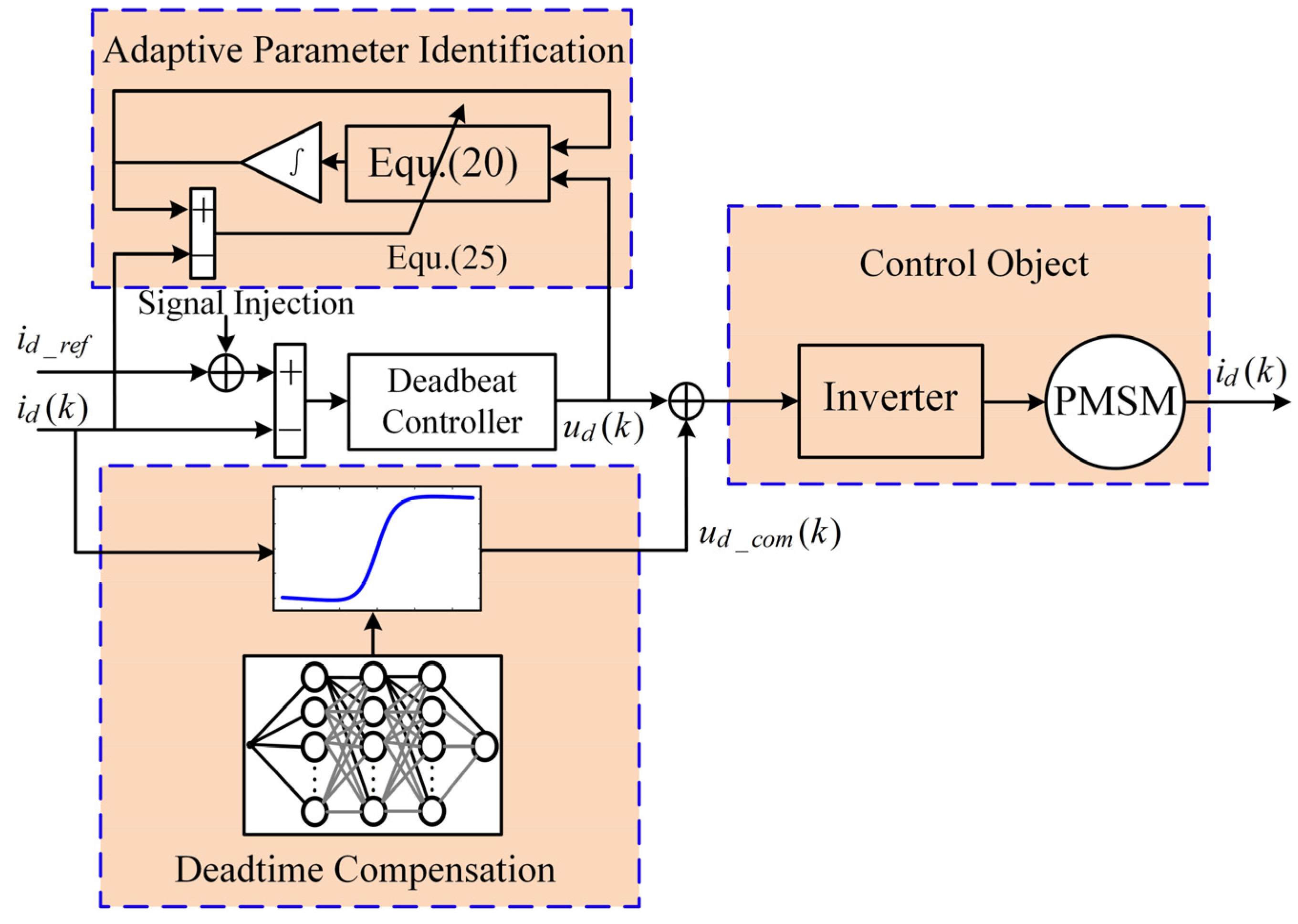
4. Online Parameter Identification

Since the q-axis current will affect the electromagnetic torque, if the parameters are identified through the q-axis current, the motor torque may be disturbed. Since the control objects in this paper are surface-mounted permanent magnet synchronous motors; that is, the inductance of the dq-axis is equal. Therefore, in this paper, the d-axis inductance is identified by using the d-axis voltage equation. The equation is as follows:

$${\dot{i}}_d={\lambda }_1{u}_d+{\omega }_e{i}_q-i_d{\lambda }_2$$

(18)

In Equation (18), ${\lambda }_1=\raisebox{1ex}{$1$}\!\left/ \!\raisebox{-1ex}{$L_m$}\right.$, ${\lambda }_2=\raisebox{1ex}{$R_s$}\!\left/ \!\raisebox{-1ex}{$L_m$}\right.$. L_m is the d-axis inductance, and R_s is the resistance. The online parameter observer can be built from Equation (18) as:

$${\dot{\widehat{i}}}_d={\widehat{\lambda }}_1{u}_d+{\omega }_e{i}_q-{\widehat{i}}_d{\widehat{\lambda }}_2$$

(19)

In Equation (19), ${\widehat{\lambda }}_1$ and ${\widehat{\lambda }}_2$ are the estimation values of λ₁ and λ₂. Subtracting Equation (19) from Equation (18) obtains:

$${\dot{\tilde{i}}}_d={\tilde{\lambda }}_1{u}_d-{\tilde{i}}_d{\lambda }_2-{\widehat{i}}_d{\tilde{\lambda }}_2$$

(20)

In Equation (20), ${\tilde{i}}_d=i_d-{\widehat{i}}_d$, ${\tilde{\lambda }}_1={\lambda }_1-{\widehat{\lambda }}_1$, ${\tilde{\lambda }}_2={\lambda }_2-{\widehat{\lambda }}_2$. To design an appropriate adaptive rate and ensure that the parameters can converge to the true value, the Lyapunov function is designed as follows:

$$x(t)=\frac{1}{2}{\tilde{i}}_d{}^2+\frac{1}{2p_1}{\tilde{\lambda }}_1{}^2+\frac{1}{2p_2}{\tilde{\lambda }}_2{}^2$$

(21)

In Equation (21), p₁ and p₂ are two positive real numbers. Thus, it can be derived that:

$$\dot{x}(t)={\tilde{i}}_d{\dot{\tilde{i}}}_d+\frac{1}{p_1}{\tilde{\lambda }}_1{\dot{\tilde{\lambda }}}_1+\frac{1}{p_2}{\tilde{\lambda }}_2{\dot{\tilde{\lambda }}}_2$$

(22)

Since the resistance and inductance parameters can be considered as slowly changing variables, the above formula can be simplified as:

$$\dot{x}(t)={\tilde{i}}_d{\dot{\tilde{i}}}_d-\frac{1}{p_1}{\tilde{\lambda }}_1{\dot{\widehat{\lambda }}}_1-\frac{1}{p_2}{\tilde{\lambda }}_2{\dot{\widehat{\lambda }}}_2$$

(23)

Substituting Equation (20) into Equation (23), it can be derived that:

$$\dot{x}(t)={\tilde{i}}_d({\tilde{\lambda }}_1{u}_d-{\tilde{i}}_d{\lambda }_2-{\widehat{i}}_d{\tilde{\lambda }}_2)-\frac{1}{p_1}{\tilde{\lambda }}_1{\dot{\widehat{\lambda }}}_1-\frac{1}{p_2}{\tilde{\lambda }}_2{\dot{\widehat{\lambda }}}_2$$

(24)

The adaptive laws can be designed as follows:

$$\begin{array}{l}{\dot{\widehat{\lambda }}}_1=p_{{}_1}{\tilde{i}}_d{u}_d\\ {\dot{\widehat{\lambda }}}_2=-p_{{}_2}{\tilde{i}}_d{\widehat{i}}_d\end{array}$$

(25)

Substituting Equation (25) into Equation (24), it can be derived that:

$$\begin{array}{ll}\dot{x}(t)& ={\tilde{i}}_d({\tilde{\lambda }}_1{u}_d-{\tilde{i}}_d{\lambda }_2-{\widehat{i}}_d{\tilde{\lambda }}_2)-\frac{1}{p_1}{\tilde{\lambda }}_1{p}_{{}_1}{\tilde{i}}_d{u}_d-\frac{1}{p_2}{\tilde{\lambda }}_2{p}_{{}_2}{\tilde{i}}_d{\widehat{i}}_d\\ & =-{\tilde{i}}_d{\tilde{i}}_d{\lambda }_2\le 0\end{array}$$

(26)

Therefore, the adaptive law designed as Equation (25) can ensure that the error of Equation (20) converges to zero. In addition, to ensure λ₁ and λ₂ converge to the true value requires the adaptive system Equation (19) to meet the sufficient excitation conditions, so two different sinusoidal currents of 200 and 500 Hz with 1% rated amplitude are injected into the d-axis current.

Combing with the offline deadtime compensation and online parameter identification method, the control structure is shown as Figure 6.

5. Results

To verify the validity of the algorithm, experimental verification of the proposed algorithm is carried out in this section. The parameters of PMSM are given in

Table 1. Parameters of the PMSM motor.

Parameters	Units	Values
Rated voltage Udc	V	220
Rated power P	kW	0.4
Stator resistance Rs	Ω	1.7
Rated speed n	r/min	3000
Torque T	N·m	1.27
inductance L	mH	6
Flux linkage of PM ψf	Wb	0.071
Rotational inertia J	Kg·m2	0.000029
Sampling period Ts	s	0.0001

, and the experimental platform is shown in Figure 7. Figure 7a shows the inverter board, and Figure 7b gives the motor test platform. The inverter block in the experiment is Infenion Intelligence power module IM513-L6A

• Identification of inverter nonlinearity

In this experiment, the test motor is controlled at 0 rpm, and the d-axis is kept coincident with phase A. The load current is controlled at different amplitudes, and the voltage waveform is shown as follows:

Figure 8 shows the relationship between the drain and source voltage at different load currents when the polarity of the current remains positive. It can be seen from Figure 8a that the current has no influence on the voltage characteristics during the opening process of the forward current. After the opening propagation, the current at different amplitudes reaches the bus voltage at the same time. For the turn-off process, as shown in Figure 8b, V_DS does not immediately drop to zero but slowly decreases due to the charging and discharging process of parasitic capacitance, and the decreased time is related to the phase current. The smaller the phase current is, the longer the charge and discharge time will be, and the voltage error will be generated during the turn-off process, which will lead to an increasing in the average voltage. This voltage can compensate for the voltage disturbance caused by the deadtime effect for the positive current. Figure 9 shows the process of turning on and off when the current is negative.

In Figure 9, the load current is negative, and the switch opening process is not related to the phase current amplitude, which is shown in Figure 9a. After the opening of the switch propagation, the V_DS at different current amplitudes changes to zero at the same time. In the process of switching off, the current path will first pass through the parasitic capacitance, and the charge and discharge times are related to the current amplitude. V_DS will not reach the stable value immediately, resulting in the average voltage drop, as shown in Figure 9b. Therefore, for negative phase current, the effect of parasitic capacitance increases the average voltage, and the lower the current amplitude is, the more obvious the effect of parasitic capacitance is.

To identify the nonlinear deadtime characteristics, the phase of the d-axis coincides with phase A, and a sinusoidal current was injected to phase A to make the current signal fully changed in the nonlinear interval. The d-axis voltage and phase A current are collected to identify the deadtime characteristics.

The offline neural network identification results are presented in Figure 10. Figure 10a shows the measured signal value. Since d-axis and phase A are kept coincident at this time, the amplitude of phase A current is twice that of phases B and C’s current. By substituting i_a and u_d into the established offline neural network, deadtime characteristics can be identified, as shown in Figure 10b. The relationship between the current amplitude and deadtime voltage is given in this figure. As the current amplitude rises, the deadtime voltage tends to be constant, showing a saturation characteristic. When the current amplitude is small, the deadtime voltage drop is approximately linear to the current. Figure 10b also verifies the influence of parasitic capacitance on deadtime compensation; that is, the lower the current amplitude is, the lower the deadtime disturbance voltage is. The convergence process of the identification error is shown in Figure 10c. In Figure 10c, the iteration error decreases with the increase in iteration times, and the iteration stops after the convergence condition is reached, indicating that the designed cut-off condition, Equation (17), can ensure that the error converges to a smaller value. Based on the relationship between error voltage and current in Figure 10b, the compensation voltage and the measured voltage error are calculated, which is shown in Figure 10d. In this figure, u_e represents the deadtime characteristics identified by offline neural network, and u_m represents the actually measured deadtime characteristics. As can be seen from Figure 10d, the identification voltage can follow the actual deadtime voltage in both the dynamic process and the steady process well, and the overall error between the two is less than 0.1 V. Therefore, the proposed offline neural network identification method can be used to compensate the deadtime effect at any current amplitude.

2.

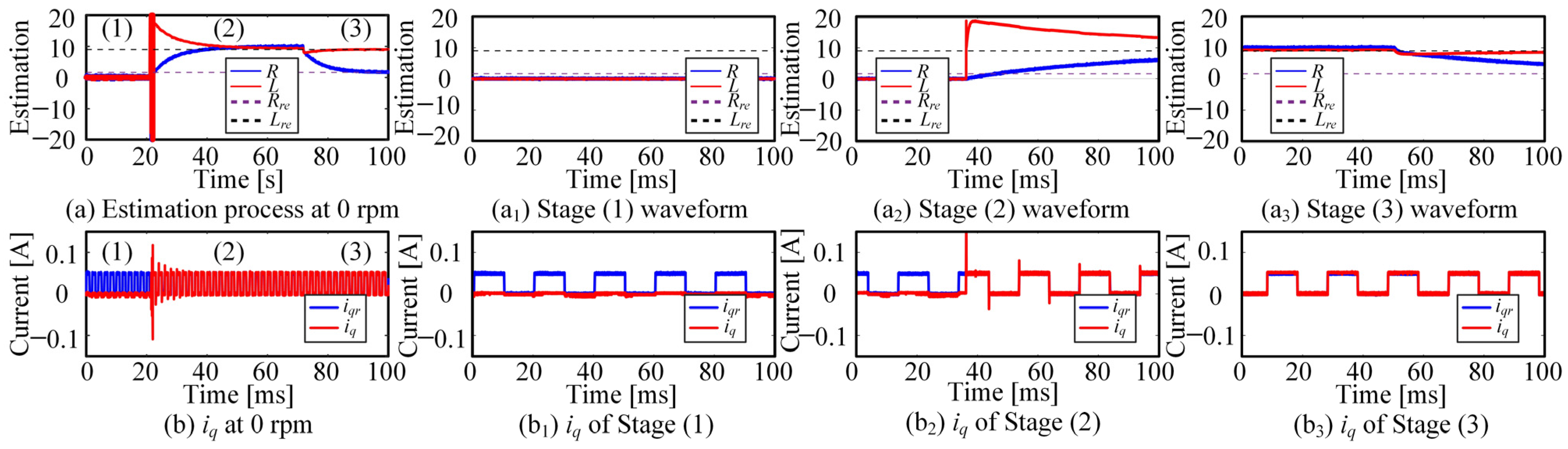
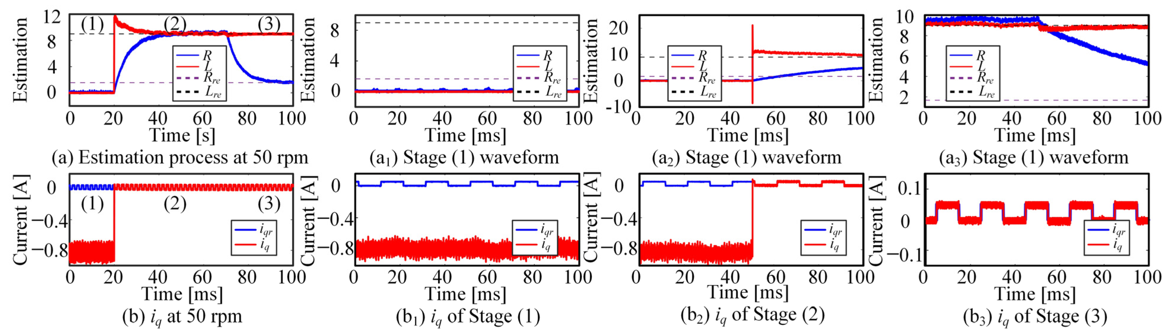
Identification of PMSM parameters

To verify the effectiveness of the parameter identification algorithm in the low-speed region, the parameter identification algorithm was verified at different speeds. The accuracy of the parameters was verified by the response of the current for the square wave reference with the amplitude of 0.05 A at the q-axis. The tested motor is driven by a commercial servo motor and controlled in constant speed mode.

In the identification process, the whole process is divided into three stages. The first stage is the initial parameter stage, and both λ₁ and λ₂ are set to 1. In this stage, adaptive parameter identification is not enabled. In Stage (2), parameter identification was enabled, and sine waves of 200 and 500 Hz with an amplitude of 0.025 A were injected into the d-axis; Stage (3) enables the proposed offline deadtime compensation algorithm.

In Figure 11, R represents the identification resistance in ohms, L represents the identification inductance in millihenry, R_re is the real motor inductance in ohms and L_re represents the real inductance in millihenry. In Figure 11a, the variation trend of the parameters in the Stages (1), (2) and (3) at zero velocity is given. In Figure 11a₁–a₃, the corresponding transient waveform at different stages is given. In Figure 11b, the tracking of the q-axis current on the given square wave is given. (1), (2) and (3) in this figure correspond to the three parameter change stages in Figure 11a. In addition, the transient process of the q-axis current at each stage is displayed in Figure 11b₁–b₃. It can be seen from stage (1) in Figure 11a,a₁ that when parameter identification is not enabled, the resistance and inductance values in the controller remain at 0, so the q-axis current in Stage (1) of Figure 11b will not follow the reference square wave current. At Stage (2) of Figure 11a, the online parameter identification strategy is enabled. Currently, the inductance rapidly converges to the true value, but the resistance converges to the wrong parameter due to the influence of the inverter deadtime. It can also be seen from Figure 11a₂ that the inductance parameter converges to the true value after a short step, but the resistance parameter error increases gradually. At this time, the corresponding current response is shown in Figure 11b₂. Since the inductance parameter is larger than the true value at the beginning, the q-axis current has a large overshoot during the step. However, as the inductance is closer to the true value, the overshoot decreases. When the offline deadtime compensation model is enabled in Stage (3) of Figure 11a, the inductance parameters remain at the true value, while the resistance parameters gradually converge to the true value from the previous error steady-state value. At this time, the current response of the q-axis is shown in Figure 11b₃. When the resistance value is too large, the feedback current i_q is greater than the given value i_qr, resulting in steady-state error. With the convergence of the resistance values, the q-axis current can be tracked without overshoot and static error.

Figure 12 shows the parameter identification results at the speed of 50 rpm, and the whole identification process is divided into three stages. In Stage (1), the resistance and inductance parameters are not accurate. Therefore, the q-axis current is not controlled at this time which is shown in Stage (1) of Figure 12a,b₁. After the online parameter identification is adopted in Stage (2), the inductance converges to the true value after the transient step, but the resistance parameter converges to the wrong value. Currently, the q-axis current begins to track the current reference after the inductance converges. The parameter convergence waveform is shown in Stage (2) of Figure 12a,a₂. The current tracking waveform is shown in Figure 12b₂. In Stage (3), the offline deadtime compensation is enabled, and the resistance parameters converge to the real value rapidly. Further, the fluctuation of inductance parameters decreases and becomes more stable. The waveform is shown in Stage (3) of Figure 12a. At this time, the steady-state fluctuation of the q-axis current is smaller as the resistance converges and is shown in Figure 12b₃.

Figure 13 shows the motor parameter identification results at 100 rpm. After parameter identification is enabled in Stage (2), the inductance parameters converge to the true value while the resistance parameters converge to the wrong value, and the q-axis current can track the reference value. After offline deadtime compensation is enabled in Stage (3), the resistance converges to the true value. The detailed analysis is the same as that at zero speed and 50 rpm.

6. Discussion

To identify the parameters at the low-speed region, the influence of the deadtime effect considering the parasitic capacitance is researched. Because of the nonlinear characteristics of the deadtime effect, an offline neural network is proposed to identify the deadtime voltage. Combined with the deadtime compensation method, an online parameter identification algorithm is proposed based on a model adaptive reference strategy. From the experimental results, the effectiveness of the proposed method is verified.

7. Conclusions

Through experimental and theoretical verification, the identification results of the neural network can track the actual voltage error well, and according to the identified current and voltage characteristics, the nonlinear characteristics of the system can be observed, which verifies the theoretical correctness of this paper. Using the proposed deadtime compensation method, decoupling of the deadtime voltage and resistance voltage drop is achieved, realizing the online identification of resistance parameters and inductance parameters in the low-speed region. Using the online identification algorithm, the deadbeat dynamic performance of the current loop without the need for initial parameters is realized. To sum up, through the deadtime compensation strategy and parameter online identification strategy proposed in this paper, the high dynamic and high robust operation of the current loop for the servo system in the low-speed region is realized.

References

1. Xu, Y.; Li, S.; Zou, J. Integral Sliding Mode Control Based Deadbeat Predictive Current Control for PMSM Drives With Disturbance Rejection. IEEE Trans. Power Electron. 2021, 37, 2845–2856. [Google Scholar] [CrossRef]
2. Wu, C.; Zhao, Y.; Sun, M. Enhancing Low-Speed Sensorless Control of PMSM Using Phase Voltage Measurements and Online Multiple Parameter Identification. IEEE Trans. Power Electron. 2020, 35, 10700–10710. [Google Scholar] [CrossRef]
3. Zhao, H.; Wu, Q.J.; Kawamura, A. An accurate approach of nonlinearity compensation for VSI inverter output voltage. IEEE Trans. Power Electron. 2004, 19, 1029–1035. [Google Scholar] [CrossRef]
4. Guha, A.; Narayanan, G. Small-Signal Stability Analysis of an Open-Loop Induction Motor Drive Including the Effect of Inverter Deadtime. IEEE Trans. Ind. Appl. 2015, 52, 242–253. [Google Scholar] [CrossRef]
5. Wang, L.; Xu, J.; Chen, Q.; Geng, X.; Lin, K. Analysis of the Effect of the Parasitic Capacitance of Switch Devices on Current Distortions of Voltage Source Rectifier. In Proceedings of the 2021 IEEE 16th Conference on Industrial Electronics and Applications (ICIEA), Chengdu, China, 1–4 August 2021; pp. 666–671. [Google Scholar] [CrossRef]
6. Sun, W.; Gao, J.; Liu, X.; Yu, Y.; Wang, G.; Xu, D. Inverter Nonlinear Error Compensation Using Feedback Gains and Self-Tuning Estimated Current Error in Adaptive Full-Order Observer. IEEE Trans. Ind. Appl. 2016, 52, 472–482. [Google Scholar] [CrossRef]
7. Munoz-Garcia, A.; Lipo, T.A. On-line dead time compensation technique for open-loop PWM-VSI drives. In Proceedings of the APEC ‘98 Thirteenth Annual Applied Power Electronics Conference and Exposition, Anaheim, CA, USA, 15–19 February 1998; pp. 95–100. [Google Scholar] [CrossRef] [Green Version]
8. Gong, L.M.; Zhu, Z.Q. Modeling and compensation of inverter nonlinearity effects in carrier signal injection-based sensorless control methods from positive sequence carrier current distortion. In Proceedings of the 2010 IEEE Energy Conversion Congress and Exposition, Atlanta, GA, USA, 12–16 September 2010; pp. 3434–3441. [Google Scholar] [CrossRef]
9. Ahmed, S.; Shen, Z.; Mattavelli, P.; Boroyevich, D.; Karimi, K.J. Small-Signal Model of Voltage Source Inverter (VSI) and Voltage Source Converter (VSC) Considering the DeadTime Effect and Space Vector Modulation Types. IEEE Trans. Power Electron. 2016, 32, 4145–4156. [Google Scholar] [CrossRef]
10. Huang, Q.; Niu, W.; Xu, H.; Fang, C.; Shi, L. Analysis on dead-time compensation method for direct-drive PMSM servo system. In Proceedings of the 2013 International Conference on Electrical Machines and Systems (ICEMS), Busan, Korea, 26–29 October 2013; pp. 1271–1276. [Google Scholar] [CrossRef]
11. Shen, Z.; Jiang, D. Dead-Time Effect Compensation Method Based on Current Ripple Prediction for Voltage-Source Inverters. IEEE Trans. Power Electron. 2018, 34, 971–983. [Google Scholar] [CrossRef]
12. Kim, S.-Y.; Lee, W.; Rho, M.-S.; Park, S.-Y. Effective Dead-Time Compensation Using a Simple Vectorial Disturbance Estimator in PMSM Drives. IEEE Trans. Ind. Electron. 2009, 57, 1609–1614. [Google Scholar] [CrossRef]
13. Wang, Q.; Zhao, N.; Wang, G.; Zhao, S.; Chen, Z.; Zhang, G.; Xu, D. An Offline Parameter Self-Learning Method Considering Inverter Nonlinearity With Zero-Axis Voltage. IEEE Trans. Power Electron. 2021, 36, 14098–14109. [Google Scholar] [CrossRef]
14. Lee, D.-H.; Ahn, J.-W. A Simple and Direct Dead-Time Effect Compensation Scheme in PWM-VSI. IEEE Trans. Ind. Appl. 2014, 50, 3017–3025. [Google Scholar] [CrossRef]
15. Kang, M.-C.; Lee, S.-H.; Yoon, Y.-D. Compensation for inverter nonlinearity considering voltage drops and switching delays of each leg’s switches. In Proceedings of the 2016 IEEE Energy Conversion Congress and Exposition (ECCE), Milwaukee, WI, USA, 18–22 September 2016; pp. 1–7. [Google Scholar] [CrossRef]
16. Hoang, K.D.; Aorith, H.K.A. Online Control of IPMSM Drives for Traction Applications Considering Machine Parameter and Inverter Nonlinearities. IEEE Trans. Transp. Electrif. 2015, 1, 312–325. [Google Scholar] [CrossRef] [Green Version]
17. El-Daleel, M.; Mahgoub, A. Accurate and simple improved lookup table compensation for inverter dead time and nonlinearity compensation. In Proceedings of the 2017 Nineteenth International Middle East Power Systems Conference (MEPCON), Cairo, Egypt, 19–21 December 2017; pp. 1358–1361. [Google Scholar] [CrossRef]
18. Urasaki, N.; Senjyu, T.; Kinjo, T.; Funabashi, T.; Sekine, H. Dead-time compensation strategy for permanent magnet synchronous motor drive taking zero-current clamp and parasitic capacitance effects into account. IEE Proc.-Electr. Power Appl. 2004, 152, 845–853. [Google Scholar] [CrossRef]
19. Zhang, Z.; Xu, L. Dead-Time Compensation of Inverters Considering Snubber and Parasitic Capacitance. IEEE Trans. Power Electron. 2013, 29, 3179–3187. [Google Scholar] [CrossRef]
20. Wang, D.; Zhang, P.; Jin, Y.; Wang, M.; Liu, G.; Wang, M. Influences on Output Distortion in Voltage Source Inverter Caused by Power Devices’ Parasitic Capacitance. IEEE Trans. Power Electron. 2018, 33, 4261–4273. [Google Scholar] [CrossRef]
21. Shen, G.; Yao, W.; Chen, B.; Wang, K.; Lee, K.; Lu, Z. Automeasurement of the Inverter Output Voltage Delay Curve to Compensate for Inverter Nonlinearity in Sensorless Motor Drives. IEEE Trans. Power Electron. 2013, 29, 5542–5553. [Google Scholar] [CrossRef]
22. Zhou, Z.; Xia, C.; Yan, Y.; Wang, Z.; Shi, T. Disturbances Attenuation of Permanent Magnet Synchronous Motor Drives Using Cascaded Predictive-Integral-Resonant Controllers. IEEE Trans. Power Electron. 2017, 33, 1514–1527. [Google Scholar] [CrossRef]
23. Liu, T.; Li, Q.; Tong, Q.; Zhang, Q.; Liu, K. An Adaptive Strategy to Compensate Nonlinear Effects of Voltage Source Inverters Based on Artificial Neural Networks. IEEE Access 2020, 8, 129992–130002. [Google Scholar] [CrossRef]
24. Qiu, T.; Wen, X.; Zhao, F.; Feng, Z. Adaptive Linear Neuron Based Dead Time Effects Compensation Scheme. IEEE Trans. Power Electron. 2016, 31, 2530–2538. [Google Scholar] [CrossRef]
25. Urasaki, N.; Senjyu, T.; Uezato, K.; Funabashi, T. Adaptive Dead-Time Compensation Strategy for Permanent Magnet Synchronous Motor Drive. IEEE Trans. Energy Convers. 2007, 22, 271–280. [Google Scholar] [CrossRef]
26. Hwang, S.-H.; Kim, J.-M. Dead Time Compensation Method for Voltage-Fed PWM Inverter. IEEE Trans. Energy Convers. 2010, 25, 1–10. [Google Scholar] [CrossRef]
27. Tang, Z.; Akin, B. A New LMS Algorithm Based Deadtime Compensation Method for PMSM FOC Drives. IEEE Trans. Ind. Appl. 2018, 54, 6472–6484. [Google Scholar] [CrossRef]
28. Lee, J.-H.; Sul, S.-K. Inverter Nonlinearity Compensation Through Deadtime Effect Estimation. IEEE Trans. Power Electron. 2021, 36, 10684–10694. [Google Scholar] [CrossRef]
29. Lee, J.; Yoo, J.; Sul, S.-K. Stator Resistance Estimation using DC Injection Robust to Inverter Nonlinearity in Induction Motors. In Proceedings of the 2020 IEEE Energy Conversion Congress and Exposition (ECCE), Detroit, MI, USA, 11–15 October 2020; pp. 2425–2430. [Google Scholar] [CrossRef]
Figure 1. The deadtime effect considering the parasitic capacitance under positive current. (a) The equivalent circuit. (b) The gate signal. (c) The drain-to-source voltage.
Energies 15 04314 g001
Figure 2. The deadtime effect considering the parasitic capacitance under negative current. (a) The equivalent circuit. (b) The gate signal. (c) The drain-to-source voltage.
Energies 15 04314 g002
Figure 3. The offline identification equivalent circuit model.
Energies 15 04314 g003
Figure 4. Offline neural network identification process.
Energies 15 04314 g004
Figure 5. Neural network equivalent model.
Energies 15 04314 g005
Figure 6. Control structure.
Energies 15 04314 g006
Figure 7. The experiment platform. (a) Inverter board. (b) The motor platform.
Energies 15 04314 g007
Figure 8. Influence of positive current with different amplitudes on the drain source voltage.
Energies 15 04314 g008
Figure 9. Influence of negative current with different amplitudes on the drain source voltage.
Energies 15 04314 g009
Figure 10. Influence of negative current with different amplitudes on the drain source voltage.
Energies 15 04314 g010
Figure 11. The parameter identification results at 0 rpm.
Energies 15 04314 g011
Figure 12. The parameter identification results at 50 rpm.
Energies 15 04314 g012
Figure 13. The parameter identification results at 100 rpm.
Energies 15 04314 g013