Abstract
In this paper, a method of power system equipment recognition based on image processing is proposed. Firstly, we carry out wavelet transform on the sound signal of power system equipment collected from the site, and obtain the wavelet coefficient–time diagram. Then, the similarity of wavelet coefficients–time images of different equipment and the same equipment in different periods is calculated, which is used as the basis of the feasibility of image recognition. Finally, we select the HOG features of the image, and classify the selected features using SVM classifier. The method proposed in this paper can accurately identify and classify power system equipment through sound signals, and is different from the traditional method of classifying sound signals directly. The advantages of image processing can be effectively utilized through image processing to avoid the limitations of sound signal processing.
1. Introduction
With the gradual development of large-scale, integrated, highly automated and intelligent power system equipment, not only are rapid economic benefits introduced, but also the risk of great loss caused by sudden equipment failure is increased. Therefore, the comprehensive, timely and accurate monitoring of the power system equipment health status ensures the stable operation of equipment, reduces the accidental shutdown rate and has a high investment–income ratio. To this end, researchers carried out systematic research on temperature, vibration, image and other aspects of various power system equipment, and obtained effective information characteristics [1,2,3]. In addition, artificial intelligence [4], deep learning [5] and neural network [6] have been used to realize fault monitoring of equipment.
According to Kafeel et al. [7], current, sound and vibration are the most commonly monitored parameters. In Ribeiro et al. [8] a hydro-generator current-monitoring system is proposed and the fast Fourier transform (FFT) is applied to the Parker transform of the current. Song et al. [9] used the bin method, the method based on multivariate normal distribution and the Copula method to compare three Bayesian diagnosis models on account of SCADA (Supervisory Control And Data Acquisition). Li et al. [10], aiming at the problems of high-speed and long-distance transmission and greatly increasing data storage capacity, proposed a method on account of adjustable q-factor wavelet transform morphologic module analysis, including few and scattered Bayesian iterative arithmetic unite stepping pulse dictionary. Yu et al. [11] try to build a rough set with feature relationships, then use a distribution reduction arithmetic to dislodge unnecessary features and send the remaining features to a flexible naive Bayesian sorter for malfunction diagnoses. In Herp et al. [12], a method is proposed to establish a fault-diagnosis model by learning fault samples, assuming that the error features picked up from SCADA (Supervisory Control And Data Acquisition) data compliance a Gaussian distribution in the characteristic space. Wang D. [13] present a method for improving wavelet filtering by combining infographics and Bayesian inference to confirm the best wavelet argument and apply to malfunction diagnoses. In Li et al. [14], in the process of fault feature extraction, the importance of different signals is optimized by particle swarm optimization. Yu et al. [15] propose an error-feature collection means based on Mean Multigrain Decision Theory Rough Sets (MMGDTRS) and Non-Naive Bayes Classifier (NNBC). Li et al. [16] present a new first-rank Bayesian command method for predicting early failure of gear-shaft systems with locally observable degradation and random failure. A polybasic Bayesian command strategy on account of Hidden Semi-Markov Model (HSMM) is proposed. In Liu et al. [17], a state-monitoring method of rolling bearings based on hybrid generalized HMM is introduced, which uses interval value features to effectively identify and classify the state in the machine process. In Gan and Jiao [18], a malfunction diagnoses means of wavelet transform gearbox on account of ameliorated inheritance arithmetic radio frequency sorter is proposed. Li et al. [19] introduced a malfunction diagnoses means for gearboxes on account of deep radio frequency integration of aural and oscillation signals. Han and Jiang [20] use VMD to acquire eigenvectors and send them to RF for fault diagnosis. Qin [21] welded Ensemble Empirical Mode Decomposition (EEMD) and RF for malfunction diagnoses. Verellen et al. [22], aiming at the detection of bearing faults in rotating machinery, propose a non-invasive acoustic signal-monitoring system based on a sparse microphone array. Traditional vibration analysis uses accelerometers, which are touch sensors that need to be attached to the component under investigation. Smieja et al. [23] proposed an interesting non-contact vibration monitoring method in which image processing is used. Cao et al. [24] proposed a pipeline robot fault diagnosis system based on sound-signal recognition, which transmits the sound signal collected by the storage sensor to the upper computer for fault diagnosis, and the test has achieved good results. Suman et al. [25] proposed an acoustic signal mode-determination algorithm based on adaptive Kalman filtering and MFCC, which can effectively detect vehicle health status by using acoustic signals to detect vehicle mechanical faults. Rakesh Kumar et al. [26] established a rainforest species audio signal-recognition model based on the combination of long short-term memory (LSTM) and convolutional neural network (CNN). The models are combined to achieve a high-accuracy, low-loss detection method. Zhuo et al. [27] proposed a program for on-line diagnosis of steel truss structures using sound signals, and proposed an improved offline database-guided response power and phase transformation method. Experiments show that this method can achieve accurate positioning in strong noise environments, and the amount of computation is smaller.
In this paper, the audio-signal monitoring of power equipment is studied deeply. At present, most sound-signal-processing technologies are based on the receiving frequency range of human ear mechanism. The existing technologies lead to many high- and low-frequency sound signals beyond the range of the human ear not being effectively utilized, resulting in the loss of a large number of effective signal data. However, even if the whole-frequency-band signal-extraction method is adopted, the characteristics of signals are difficult to separate from each other, and the extraction is difficult. The essential reason for these problems is that the coverage of sound signals is extremely wide, so the difficulty of recognition is greatly increased [28]. It can be seen that the traditional sound signal-processing technology has considerable limitations. In order to solve this problem, we took another analytical way of thinking: no longer the traditional method, but the audio-processing problem transferred to the field of image processing. As a result, this paper proposes a power equipment based on wavelet transform voice-fault identification analysis method, in which the access to the audio signal by DWT abstracts the wavelet coefficient of sound. The time-frequency diagram and wavelet coefficient diagram of sound signal are output, and the method of machine learning [29] is applied to analyze sound information from the perspective of image texture. In this method, the whole frequency band of sound signal is extracted without any filtering, and then the sound signal is translated into image processing, which can effectively avoid the loss of information data and make use of the advantages of image recognition for classification.
2. Audio Signal Analysis Based on Wavelet Transform
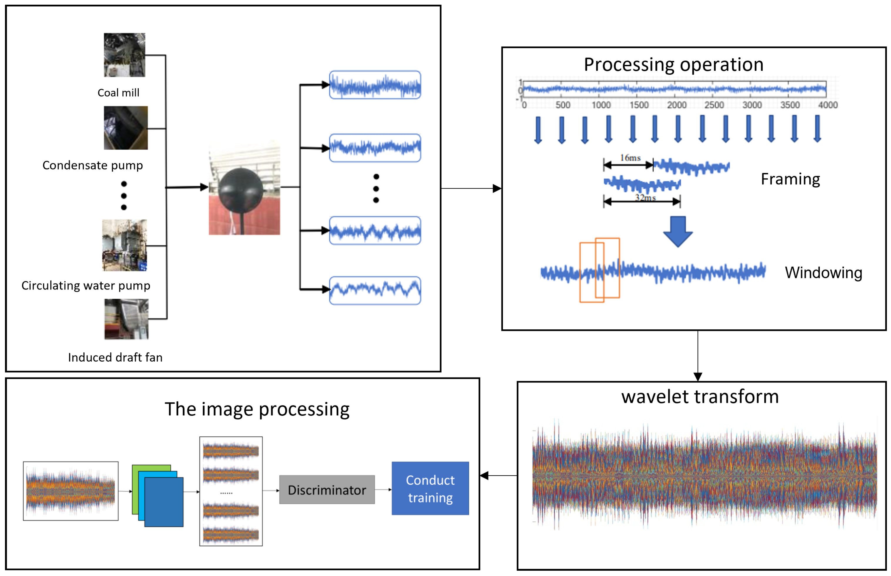
The overall structure of the research idea is shown in Figure 1. This paper studies the feature extraction method of six kinds of power equipment sounds collected by a 96-channel handheld audio imager. Firstly, we can analyze the audio pre-processing method based on Wavelet and Hamming window, and then we can obtain the audio pre-processing device with different image segmentation coefficients based on Wavelet and Hamming window, and then we can obtain the audio pre-processing device with different image segmentation coefficients; finally, based on this result, we use HOG + SVM method to classify and predict different devices, and find that it has a high recognition rate.
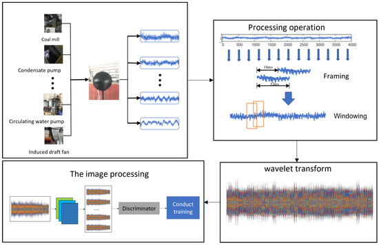
Figure 1.
The overall idea of the experimental process. The figure includes the power equipment sound-field-acquisition module, the sound signal preprocessing module, the wavelet transform output image module and the image-processing module.
- Preprocessing: the digital strainer is used to preemphasize the audio signal, determine the frame length and frame shift of each sound signal, and the Hamming window is used to filter the sound signal by framing and windowing to obtain multi-frame sound signals;
- Wavelet analysis: by obtaining separate sound signal samples of power equipment through preprocessing operation, we can analyze the characteristics of the sound signal, select an appropriate wavelet function to carry out wavelet transform on the sound signal, and obtain the time wavelet coefficient diagram of each audio signal sample;
- Image processing: considering that the wavelet coefficient image obtained in the above steps contains a large number of image features, this study first uses SSIM (Structural Similarity) image processing method to calculate the similarity between wavelet coefficient images of sound signals of different devices and the same device, so as to verify the feasibility of image classification.
- HOG + SVM: extract the hog feature of the obtained wavelet coefficient image, and substitute the extracted feature into the SVM classifier for multi-classification training, so as to achieve the purpose of classification and prediction of the existing image.
2.1. Sound Signal Preprocessing
The voice signals collected by the sound imager may have problems such as aliasing, high-order harmonic distortion and high frequency. Before analyzing the sound signals of field equipment, we carry out pre-weighting, framing, windowing and other preprocessing operations so that the signals procured by pursuant voice processing are more consistent and smooth as far as possible, allowing us to afford high-quingity parameters for signal parameter collection and further sound signal processing quality. The specific steps of sound signal preprocessing are as follows:
- Slice. In order to unify the duration of the sound sample, the sound signal of the whole section of audio is segmented into 1 s as a sound sample;
- Pre-emphasis. In order to flatten the spectrum of the sound signal, the spectrum can be calculated with the same structural return loss in the low-frequency to high-frequency band, and the sound signal of each sample is pre-emphasized. Pre-emphasis processing means that the sound signal passes through a high clear strainer:where in 0.9 < < 1.0, is taken as 0.97 in this paper.
- Normalization. Normalize the spectrum of the preprocessed sound signal to reduce the difference in the frequency range of different types of sound:
- Framing and windowing. The sound signal is stable in a short time. The short-time length is generally 10–30 ms. In order to facilitate feature analysis, the sound signal needs to be processed in frames. For purpose of ensuring the smooth conversion between two adjacent frames, the frame signal needs to be superimposed, and then each frame is multiplied by a window function of a certain length for windowing and filtering. In this paper, Hamming window is adopted, and the window function is shown in Formula (3):
2.2. Feature Extraction of Audio Signal Based on Wavelet Transform
Wavelet transform is an important time-frequency analysis approach that combines the time-domain characteristics and frequency-domain characteristics of signals.
2.2.1. Definition of Wavelet Function
The application of wavelet analysis in signal and picture compression is a crucial side of the application of wavelet analysis. It has the characteristics of high compression ratio and fast compression speed. After compression, it can not only keep the traits of the signal and image unvaried, but also resist the interference in transmission. The definition formula is as follows:
Take the function of the basic wavelet as the displacement b, and make the inner product with the signal to be analyzed under different scales a, with the transformation of a, b the wavelet transform has the traits of multi-resolution.
2.2.2. Wavelet Sequence
, is called a basic wavelet and mother wavelet, where refers to the mean square integrable space. Wavelet must meet:
This is also the meaning of “wavelet”. After scaling and translating the generating function, the wavelet sequence can be obtained:
(a, b ∈R, a≠ 0) a, b where a, b is the expansion factor and translation factor, respectively.
2.3. SSIM-Based Image Processing Method
2.3.1. Definition
Unartificial images have a sehr hoch configuration, especially in the case of spatial similarity, there is a high associations between the pixels of the image. Such associations port crucial information about the configuration of objects in the optical scenario. What we are talking about is finding a more straight method to contradistinguish the configuration of a fuzzy image with that of a reference image.
Structural similarity is a measure of how similar two images are. The SSIM value is between 0 and 1, and the larger its value, the smaller the difference between the images. The definition of SSIM is as in Equation (1) Structural similarity. From the standpoint of image formation, configurational information is defined as a reflection scene that is isolated of brightness and contrast, and the image is modeled by three different factors: brightness, contrast and structure.
Function definition:
where , , > 0.
The measure of similarity can be realized by the SSIM measuring system, which can be constituted of three comparison elements of brightness, contrast and structure. Next, we define three contrast functions:
Brightness contrast function:
Contrast function:
Structural contrast function:
For the above formula, , , stand for the whole pixels of the picture; , , stand for the criterion differences of picture pixel value; stand for the convariance of x, y; , , stand for constants. This is for the purpose of eliminating system fault when the denominator is 0. In practical application, = = = 1, = 0.5.
2.3.2. Application of SSIM
In image mass evaluation, obtaining the SSIM index of a certain part is better than all. First, the statistical features of images are generally disproportionally distributed i then room; second, image deformation varies with the room; third, under standard visual interval, people can centre around one area of the image, therefore the separate processing of a certain part is more in line with the scope of human vision; fourth, the local quality detection can obtain the mapping matrix of image spatial quality changes, and the results can be used for other applications.
Therefore, in the formula above, , , both add an 8 × 2 square window and traverse the whole image by every pixels. At every procedure of the computation, , , and SSIM values ground on the pixels in the window. Finally, an SSIM index mapping matrix is procured, which is composed of certain part SSIM indexes. However, plain-add window will lead to terrible “blocking” impression of the mapping matrix. To resolve the conundrum, we use the 11 × 11 meristic Gaussian weighing function as the weighing window, with a par differences of 1.5, and
Then the approximated value of , , is voiced as:
Using this windowing means, the mapping matrix can show the capabilities of certain part isotropy, and then use the evenness SSIM index as the evaluation quality of the entire image:
In the above, x, y are images, , are the locations of certain part SSIM index in the mapping, M, N are the number of local windows.
2.4. HOG Feature Extraction Algorithm
Histogram of Oriented Gradient (HOG) feature is a kind of descriptor that uses computer vision and image processing technology to detect object features. Image features are extracted by calculating and statistical histogram of directional gradient in a specific area of the image. The incorporation of Hog feature extraction and SVM classifier has been diffusely applied in the field of image identification.
Feature Extraction Process
(1) Detection window: Hog cut apart the image through window and block. Mathematically process the pixel values of an area in an image in units of cells. Here, we first introduce the concepts of window, block and cell and the relationship between them.
- Window: divide the image into multiple identical windows according to a certain size and slide;
- Block: divide each window into several same blocks according to a certain size and slide;
- Cell: each window is divided into multiple identical cells according to a certain size, which belong to the feature extraction unit and remain stationary.
(2) Normalized images: Normalization includes gamma and color room normalization. Normalizing the whole image can effectively reduce the influence of lighting conditions. Normalization can also avoid the large proportion of certain part external exposure contribution in picture grain intensity. Standard Gamma compression formula:
takes values based on the effect.
(3) Calculated gradient: Firstly, the gradient value in the horizontal and vertical coordinate orientation is calculated, and the gradient orientation is calculated according to the calculated gradient value. The formula is as follows:
For the two formulas , , separately stand for the aclinic gradient, perpendicular gradient and pixel value at a specific pixel point of the collected image. The gradient value of amplitude and gradient orientation at pixel (x, y) are:
(4) Constructing gradient column diagram: The orientation division is determined by bins (number of divisions). Generally, bins takes 9, and the gradient orientation is cut apart into 9 intervals.
(5) Cell-normalized gradient histogram in the block: the increasing range of gradient intensity is greatly affected by local illumination and foreground–background contrast, so normalization is needed.
(6) Generate hog feature vector: finally, combine all blocks to generate feature vector.
2.5. Support Vector Machines (SVM)
The supervised learning model of support vector machine and its related learning algorithm are widely used in machine learning. It can be used in classification of data and analysis of regression. When given the condition of a set of training specimens, each sample is labeled as one of two different varieties, and the SVM drill algorithm set up a model, deals the new specimens to a certain variety, and constructs an improbability binary linear classifier. The SVM training model represents all specimens as mappings of points in space, and divides the specimens with a wide and obvious gap. The new specimens are then mapped into the same room and their categories predicted.
3. Experimental Result
Firstly, select the working sound of six types of equipment under a fixed working condition collected from the power plant, the sampling frequency is 16,000 Hz, and the fixed 1 s is the cycle for segmentation; The sound sample data set information of six types of equipment is shown in Table 1:

Table 1.
Sound samples.
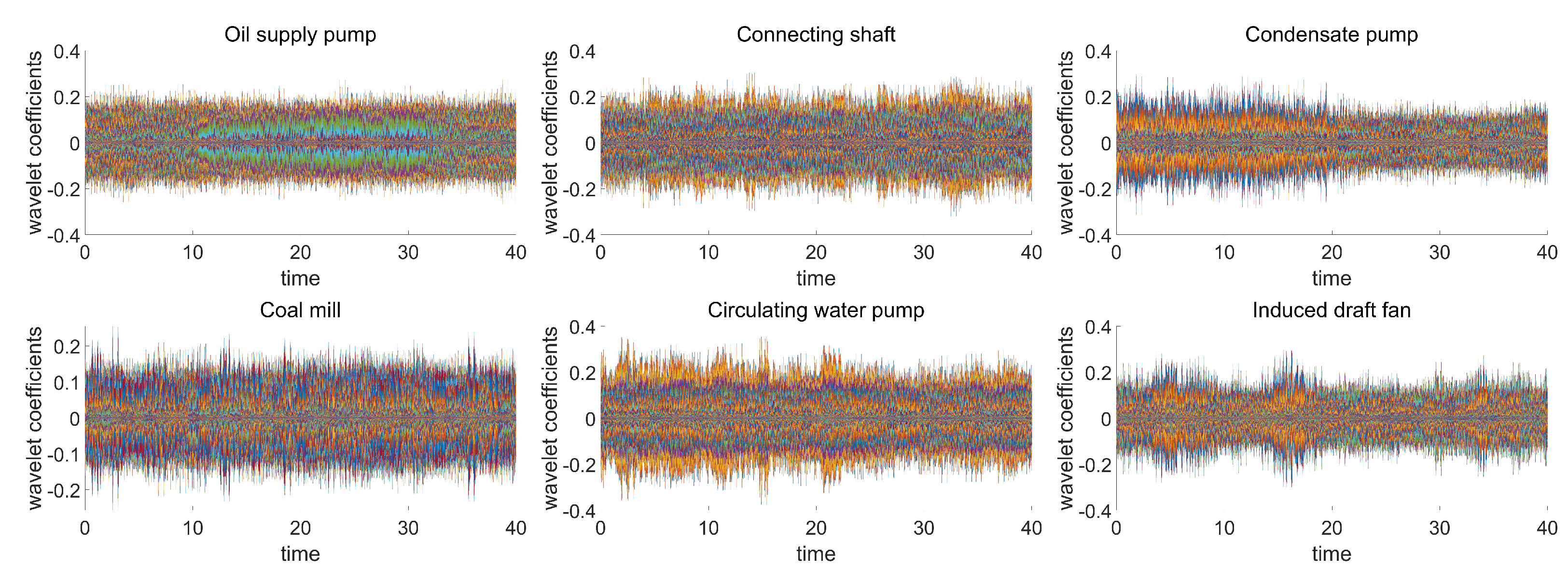
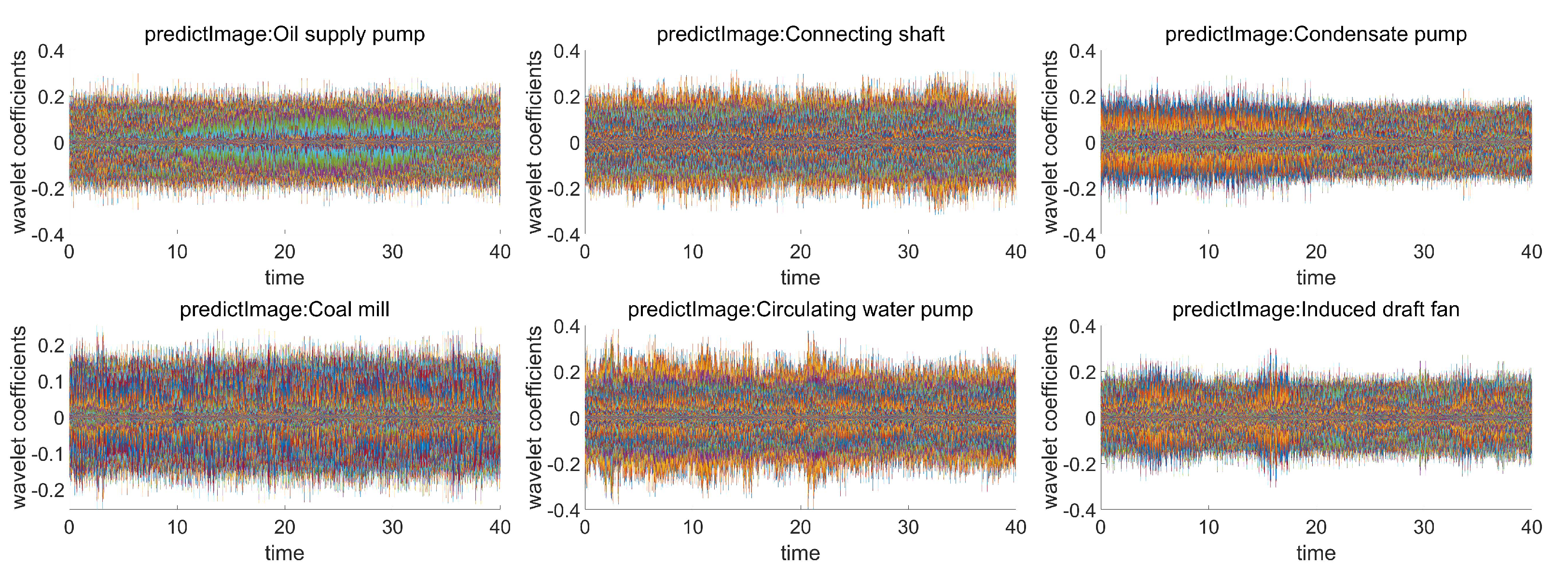
After segmentation, the 40 s audio signal of one of the six devices is selected for wavelet transform to obtain the time wavelet coefficient diagram, as shown in the following figures.
From the above image results in Figure 2, it can be seen that there are great differences in time wavelet coefficient images between different devices, and the image features are obvious. Based on this result, we intercept the other four 40 s sound data of each device and output their time wavelet coefficient diagrams. According to the obtained images, we found that the similarity of wavelet coefficient images of a device in different periods is very high, but the feature distinction between different devices is still obvious. Therefore, we took out three images of each device for intra-class and inter-class similarity comparison, and the results are shown below.
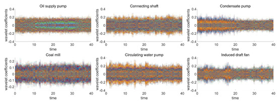
Figure 2.
Sample image. The abscissa represents time and the ordinate represents wavelet coefficients.
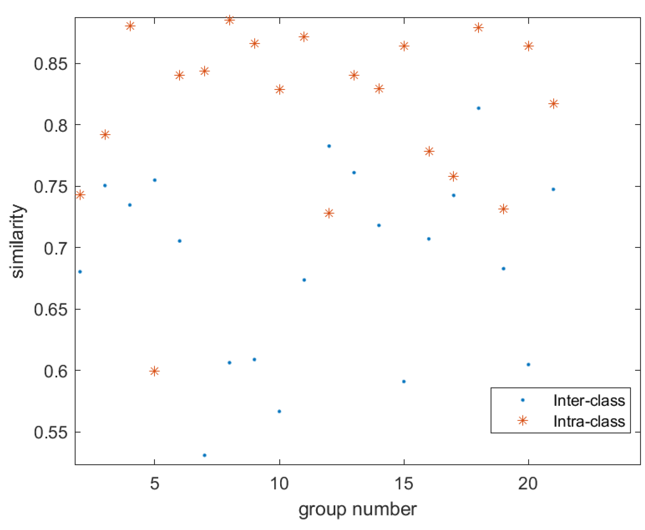
It can be seen from the Figure 3 that the signal similarity of the same equipment in different periods is generally higher than that between different equipment. Based on the above similarity-matching results, we divide the time wavelet coefficient graphs obtained by each equipment into five different time periods into two groups, one group of four graphs as the training set and the other group of one graph as the test set. In this way, a total of 24 training samples and 6 test samples of 6 types of samples are obtained. The test samples are predicted and classified by using hog feature-extraction algorithm and SVM multi-classification training. The results are shown in Table 2 and Figure 4 below.

Figure 3.
Scatter diagram of image similarity. The abscissa represents the number of sample groups, and the ordinate represents the sample similarity.
Table 2.
Classification accuracy of raw data.
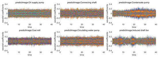
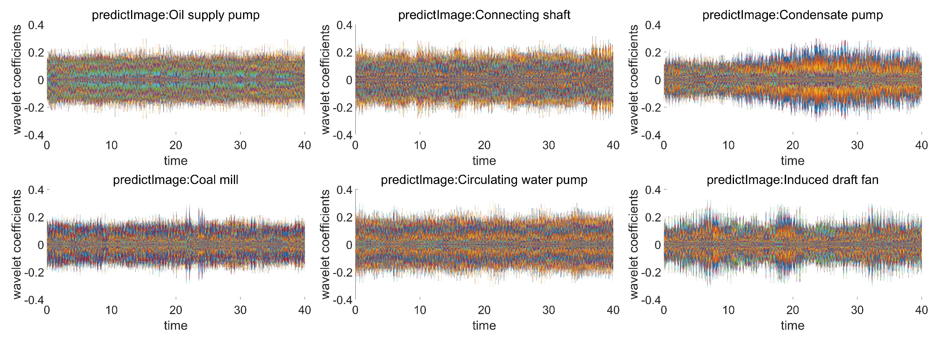
Figure 4.
Original sound classification of equipment. The abscissa represents time, and the ordinate represents wavelet coefficients.
In the field of power production, it is difficult to completely eliminate the noise interference in the extraction process of power equipment sound. Therefore, we add Gaussian white noise to the original power equipment sound signal as interference to verify the accuracy and feasibility of this method. Through experiments, we find that when 10 dB Gaussian white noise is added, the characteristics of the time wavelet coefficient diagram of each equipment are not obvious, so it is difficult to distinguish the equipment, When 20 dB Gaussian white noise is added, the characteristics of each equipment in the time wavelet coefficient diagram appear again. Therefore, we process and classify the sound signal added with 20 dB Gaussian white noise. The results are shown in Table 3 and Figure 5 below.
Table 3.
Add white noise data classification accuracy.
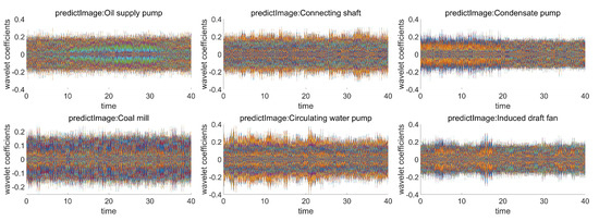
Figure 5.
Equipment classification after adding 20 dB Gaussian white noise. The abscissa represents time, and the ordinate represents wavelet coefficients.
It can be seen from the experimental results that when white Gaussian noise is affiliated to the sound signal of the equipment, the features of the images of some equipment become more difficult to distinguish, and the recognition accuracy of the image is slightly decreased, but the overall recognition accuracy is high, and the classification effect is obvious. By adding white Gaussian noise of different decibels, it is not difficult to find that noises of different decibels have different degrees of influence on the sound signal of the equipment, which is intuitively reflected in the wavelet coefficient–time diagram, making it more difficult to distinguish image features and equipment identification and classification. Compared with the traditional power equipment sound-recognition method, the advantages of the image processing-based power equipment sound-recognition method proposed in this paper lie in the use of the full frequency range of the sound signal and the more delicate feature expression. For example, a sound-recognition algorithm for substation equipment based on harmonic characteristics and vector quantization was proposed by Dong et al. [30]. The sampled sound signal of power equipment takes the 27th harmonic within 0–1300 Hz as the feature vector, so there will be a lot of noise. The sound data is not used, and the sound features are difficult to express in detail and comprehensively, which will have a certain impact on the accuracy of the results.
4. Conclusions
In this paper, aiming at the sound of six types of thermal power plant power system equipment collected from the scene, the wavelet coefficient–time map of the equipment is obtained through wavelet transformation, and the audio signal is translated into image processing. SSIM algorithm is used to calculate the same at different times and for different equipment, and the image similarity between them can draw a clear difference in terms of image characteristics, which can be used in the classification. Based on this judgment, the obtained images were classified by HOG + SVM fusion method, and 10 dB and 20 dB Gaussian white noise were added to the audio signal, respectively. It was found that noises of different decibels had different degrees of influence on the sound signal of the equipment, and the difficulty of distinguishing the features of the wavelet coefficient–time graph would be improved. Under the influence of 10 dB noise, the characteristic of the wavelet coefficient–time diagram of the equipment is not obvious and difficult to distinguish, but under the influence of 20 dB noise, the difficulty of distinguishing the characteristic of the wavelet coefficient–time diagram of equipment is increased, but the classification effect is good. The experimental results show that the recognition method of sound translation image processing, which is different from the traditional sound-recognition method, has better practical feasibility. The limitation of this paper is that the number of available audio samples is limited, and there is not enough data for training samples. Moreover, only the image obtained by wavelet transform is considered, and whether the image obtained by other methods has better feature distinguishability has not been studied deeply. In the future, we can explore more methods to express characteristic images of sound signals, and continue to study the optimal method of sound signal recognition based on image processing.
Author Contributions
Conceptualization, K.B.; methodology, K.B. and Z.C.; software, Z.C.; validation, Y.Z. (Yong Zhou); formal analysis, Y.Z. (Yong Zhou); resources, W.B.; data curation, W.B.; writing—original draft prepara-tion, Z.C.; writing—review and editing, K.B.; visualization, N.Z.; supervision, Y.Z. (Yongjie Zhai); project adminis-tration, Y.Z. (Yongjie Zhai); funding acquisition, Y.Z. (Yongjie Zhai). All authors have read and agreed to the published version of the manuscript.
Funding
This research received no external funding.
Institutional Review Board Statement
Not applicable.
Informed Consent Statement
Not applicable.
Data Availability Statement
Not applicable.
Conflicts of Interest
The authors declare no conflict of interest.
References
- Liang, L.; Liu, S.; Li, Y.; Zhong, M.; Li, Y. Distributed fault detection and isolation for power system. Int. J. Robust Nonlinear Control 2021, 32, 2143–2158. [Google Scholar] [CrossRef]
- Bakhtadze, N.; Yadikin, I. Analysis and Prediction of Electric Power System’s Stability Based on Virtual State Estimators. Mathematics 2021, 9, 3194. [Google Scholar] [CrossRef]
- Peng, J.; Yang, P.; Liu, Z.; Sun, G. Double-Fed Wind Power System Adaptive Sensing Control and Condition Monitoring. J. Sens. 2021, 2021, 5753947. [Google Scholar] [CrossRef]
- Liu, R.; Yang, B.; Zio, E.; Chen, X. Artificial intelligence for fault diagnosis of rotating machinery: A review. Mech. Syst. Signal Process. 2018, 108, 33–47. [Google Scholar] [CrossRef]
- Yang, Z.; Diao, C.; Li, B. A Robust Hybrid Deep Learning Model for Spatiotemporal Image Fusion. Remote Sens. 2021, 13, 5005. [Google Scholar] [CrossRef]
- Cao, P.; Zhang, S.; Tang, J. Preprocessing-Free Gear Fault Diagnosis Using Small Datasets With Deep Convolutional Neural Network-Based Transfer Learning. IEEE Access 2018, 6, 26241–26253. [Google Scholar] [CrossRef]
- Kafeel, A.; Aziz, S.; Awais, M.; Khan, M.A.; Afaq, K.; Idris, S.A.; Mostafa, S.M. An Expert System for Rotating Machine Fault Detection Using Vibration Signal Analysis. Sensors 2021, 21, 7587. [Google Scholar] [CrossRef]
- Ribeiro, L.C.; Bonaldi, E.L.; de Oliveira, L.E.L.; da Silva, L.E.B.; Salomon, C.P.; Santana, W.C.; Silva, J.G.B.; Lambert-Torres, G. Equipment for Predictive Maintenance in Hydrogenerators. AASRI Procedia 2014, 7, 75–80. [Google Scholar] [CrossRef]
- Song, Z.; Zhang, Z.; Jiang, Y.; Zhu, J. Wind turbine health state monitoring based on a Bayesian data-driven approach. Renew. Energy 2018, 125, 172–181. [Google Scholar] [CrossRef]
- Li, Q.; Hu, W.; Peng, E.; Liang, S.Y. Multichannel Signals Reconstruction Based on Tunable Q-Factor Wavelet Transform-Morphological Component Analysis and Sparse Bayesian Iteration for Rotating Machines. Entropy 2018, 20, 263. [Google Scholar] [CrossRef] [Green Version]
- Yu, J.; Bai, M.; Wang, G.; Shi, X. Fault diagnosis of planetary gearbox with incomplete information using assignment reduction and flexible naive Bayesian classifier. J. Mech. Sci. Technol. 2018, 32, 37–47. [Google Scholar] [CrossRef]
- Herp, J.; Ramezani, M.H.; Bach-Andersen, M.; Pedersen, N.L.; Nadimi, E.S. Bayesian state prediction of wind turbine bearing failure. Renew. Energy 2018, 116, 164–172. [Google Scholar] [CrossRef] [Green Version]
- Wang, D. An extension of the infograms to novel Bayesian inference for bearing fault feature identification. Mech. Syst. Signal Process. 2016, 80, 19–30. [Google Scholar] [CrossRef]
- Li, K.; Zhang, Q.; Wang, K.; Chen, P.; Wang, H. Intelligent Condition Diagnosis Method Based on Adaptive Statistic Test Filter and Diagnostic Bayesian Network. Sensors 2016, 16, 76. [Google Scholar] [CrossRef] [Green Version]
- Yu, J.; Ding, B.; He, Y. Rolling bearing fault diagnosis based on mean multigranulation decision-theoretic rough set and non-naive Bayesian classifier. J. Mech. Sci. Technol. 2018, 32, 5201–5211. [Google Scholar] [CrossRef]
- Li, X.; Makis, V.; Zuo, H.; Cai, J. Optimal Bayesian control policy for gear shaft fault detection using hidden semi-Markov model. Comput. Ind. Eng. 2018, 119, 21–35. [Google Scholar] [CrossRef]
- Liu, J.; Hu, Y.; Wu, B.; Wang, Y.; Xie, F.; Wang, X. A Hybrid Generalized Hidden Markov Model-Based Condition Monitoring Approach for Rolling Bearings. Sensors 2017, 17, 1143. [Google Scholar] [CrossRef] [PubMed]
- Gan, H.; Jiao, B. Fault Diagnosis of Wind Turbine’s Gearbox Based on Improved GA Random Forest Classifier. DEStech Trans. Eng. Technol. Res. 2018, 206–210. [Google Scholar] [CrossRef]
- Li, C.; Sanchez, R.V.; Zurita, G.; Cerrada, M.; Cabrera, D.; Vásquez, R.E. Gearbox fault diagnosis based on deep random forest fusion of acoustic and vibratory signals. Mech. Syst. Signal Process. 2016, 76, 283–293. [Google Scholar] [CrossRef]
- Han, T.; Jiang, D. Rolling Bearing Fault Diagnostic Method Based on VMD-AR Model and Random Forest Classifier. Shock Vib. 2016, 2016, 5132046. [Google Scholar]
- Qin, X.; Li, Q.; Dong, X.; Lv, S. The Fault Diagnosis of Rolling Bearing Based on Ensemble Empirical Mode Decomposition and Random Forest. Shock Vib. 2017, 2017, 2623081. [Google Scholar] [CrossRef]
- Verellen, T.; Verbelen, F.; Stockman, K.; Steckel, J. Beamforming Applied to Ultrasound Analysis in Detection of Bearing Defects. Sensors 2021, 21, 6803. [Google Scholar] [CrossRef] [PubMed]
- Śmieja, M.; Mamala, J.; Prażnowski, K.; Ciepliński, T.; Szumilas, Ł. Motion Magnification of Vibration Image in Estimation of Technical Object Condition-Review. Sensors 2021, 21, 6572. [Google Scholar] [CrossRef]
- Cao, H.; Yu, J.; Wang, Y.; Zhang, L.; Kim, J. A Fault Diagnosis System for a Pipeline Robot Based on Sound Signal Recognition. Sensors 2022, 22, 3275. [Google Scholar] [CrossRef] [PubMed]
- Suman, A.; Kumar, C.; Suman, P. Early detection of mechanical malfunctions in vehicles using sound signal processing. Appl. Acoust. 2022, 188, 108578. [Google Scholar] [CrossRef]
- Kumar, R.; Gupta, M.; Ahmed, S.; Alhumam, A.; Aggarwal, T. Intelligent Audio Signal Processing for Detecting Rainforest Species Using Deep Learning. Intell. Autom. Soft Comput. 2022, 31, 693–706. [Google Scholar] [CrossRef]
- Zhuo, D.; Cao, H. Damage identification of bolt connection in steel truss structures by using sound signals. Struct. Health Monit. 2022, 21, 501–517. [Google Scholar] [CrossRef]
- Birch, B.; Griffiths, C.A.; Morgan, A. Environmental effects on reliability and accuracy of MFCC based voice recognition for industrial human-robot-interaction. Proc. Inst. Mech. Eng. Part J. Eng. Manuf. 2021, 235, 1939–1948. [Google Scholar] [CrossRef]
- Liu, C.L.; Qi, W.X. Research on Fault Diagnosis Method of Wind Turbine Based on Wavelet Analysis and LS-SVM. Adv. Mater. Res. 2013, 2479, 724–725. [Google Scholar] [CrossRef]
- Li, D.S.; Zhou, Z.Q.; Zhang, C.; Du, P.; Hu, Y.R. Sound Recognition Algorithm for Power Devices Based on Substation Inspection Robots. Appl. Mech. Mater. 2014, 3360, 1139–1144. [Google Scholar] [CrossRef]
Publisher’s Note: MDPI stays neutral with regard to jurisdictional claims in published maps and institutional affiliations. |
© 2022 by the authors. Licensee MDPI, Basel, Switzerland. This article is an open access article distributed under the terms and conditions of the Creative Commons Attribution (CC BY) license (https://creativecommons.org/licenses/by/4.0/).