Abstract
The rotation precision of rotors determines the efficiency and quality of the overall aero-engine, as well as its long-term and reliable operation ability. As the terminal link of aero-engine manufacturing, the assembly is the last guarantee of precision control. Rotor assembly relates to the accurate expression of the connection form and design optimization of the assembly scheme. The existing variation model cannot adequately handle the partial parallel chain problem, ignoring the bayonet circular connector between the rotor parts, and it is still deficient in multistage gyration error control. In this paper, the partial parallel connection and multistage revolving characteristics of rotors were discussed, and a novel modeling and optimizing method for a partial parallel dimension chain was proposed. On the one hand, the variation expression of the connection features for the revolving components considering the partial parallel structure was researched. Contact point-based torsors were represented, and a system for locating points was regarded as an assembly to describe the partial parallel chain. On the other hand, the variation propagation modeling and control for the stacking of the multistage revolving components was researched. A revolution joint was introduced in the unified Jacobian–Torsor model, and a novel assembly technique for concentricity control was proposed. Therefore, a unified variation analysis and control method for rotor assembly has been developed. Experimental results show that through this method, the final concentricity variation is 0.0539 mm, far less than the 0.1595 mm of the traditional model, and is closer to the true value range of 0.030–0.040 mm. Moreover, the optimum installed angles can be calculated as 3.153 rad, 6.025 rad, and 2.590 rad, to obtain the highest concentricity of 0.040 mm, which has strong practical guiding significance.
1. Introduction
As the heart of an aircraft, the aero-engine belongs to the field of strategic high-tech equipment, which concerns national strategic security. Assembly is the terminal and key link of aero-engine manufacturing, being characterized by a high density of product, technology, manpower, and equipment [1]. General parts-level assembly requires 500–1000 sets of tooling and 30–50 kinds of processing equipment, and the assembly workload accounts for more than half of the entire engine production phase. Relative to general industrial products, the security requirements are more demanding for an aero-engine. Its assembly process is more delicate and precision control is more difficult. Taking the GE90-115B engine as an example, as one of the world’s most powerful aero-engines, its assembly success probability is less than 50% if assembled in accordance with the precision requirements that recommend that positioning error of the core cell should be not more than 0.05 mm.
As a typical example of thermo-mechanical coupled rotary machinery, an aero-engine rotor works at more than 8000 RPM. The rotor bears great inertial force, aerodynamic force, torque, and vibratory loading. If the centering scheme of the rotors is not designed properly, parts are assembled incorrectly, or the dynamic balancing test is poor, the rotors will vibrate acutely at runtime, which will directly affect the security and reliability of the aero-engine. Statistically, rotor vibration and misalignment faults account for more than 60% of all engine faults [2]. It can be said that rotor assembly is one of the most important links in the aero-engine assembly process.
For aero-engine rotor assembly, the bayonet circular connector is widely used as a typical positioning and connection mode, and thus involves the problem of a partial parallel dimension chain [3]. The composite location for multiple pairs of datum features will cause a partial connection loop on the variation propagation path, which causes difficulties for modeling and solving dimension chains. Desrochers et al. [4] distinguished and enumerated all the types of local connection joints, which were basic constitutive elements of the partial parallel structure. Zeng et al. [5] further summarized five common types of partial parallel structures on this basis. In recent years, many scholars have carried out a great deal of research on complex mechanical system assembly [6,7]. The existing variation theory for aero-engine rotor assembly mainly focuses on two aspects. One aspect focuses on solving the composite location problem for multiple pairs of datums, from the perspective of variation expression of the partial features; the other is to construct the variation propagation model of the whole engine, from the perspective of a dimension chain for assembly.
In terms of variation expression, Chavanne and Anselmetti [8] proposed a method of localization tolerancing with a contact influence. Based on this method, Zeng et al. [5] took a spiral bevel gearbox as a research object, simulating the virtual boundary surface which contained contact points of extreme variation. As a result, the feature interference problem has been adequately solved, but this method places more emphasis on the lever effect of assembly geometry. Chen et al. [9] adopted Boolean algebraic operations to improve the ability of a variation model that can effectively deal with partial parallel chains. The crank-link mechanism of an internal combustion engine was analyzed and verified. However, the solution was complicated. A large number of “intersection” and “union” operations provided a low computation efficiency. Li et al. [10] designed the flexible tooling for the disc rotor stacking by using the finite element method. The main variation sources affecting the positioning accuracy of the tooling were discussed, and a quantitative compensation method was proposed. Hong et al. [11] proposed the use of the wave finite element theory, and the band-gap characteristics of aeronautical stiffened shell parts were studied. A vibration isolation design was carried out. Andersson [12] built a finite element model of a supersonic turbine blade and discussed the influence of manufacturing variations on supersonic turbine efficiency. The main sensitive parameters affecting turbine efficiency were determined. Forslund et al. [13] studied the functional robustness of a turbine rear case relative to its assembly reference points and pointed out that geometrical variation would have a negative effect on the structural and thermal stress. However, FEM modeling is difficult, and its solving efficiency is low, which makes it suitable as an auxiliary validation method for other analytic models. Liu et al. [14,15] combined a skin model with the boundary element method and analyzed the influence of the assembly morphology error and local contact deformation on the assembly accuracy. The contact behavior at each scale of the components of the metal surfaces was studied based on a deterministic model. Sun et al. [16,17] proposed a method for the characterization and identification of the connection parameters of bolted joints based on a gradient virtual material and surrogate model, and deeply researched the morphology characterization and contact of the assembly interface based on the barycenter driven algorithm. The above methods focus on the characterization mechanism and the evaluation methods of the assembly variation at different scales, but the further exploration of three-dimensional variation propagation in complex dimensional chains is not carried out.
In terms of variation propagation, Wittwer et al. [18] linearized the nonlinear dimensional chain using the direct linearization method, which was suitable for describing the variation propagation process. However, the expression and propagation of assembly variation cannot be unified in this way. Yang et al. [19] proposed two strategies of vertical assembly and parallel assembly based on a homogeneous transformation matrix. The optimal concentricity control was carried out and the optimal installation angles were designed for aero-engine rotor stacking. Chen et al. [20] proposed a novel constraint condition establishment and optimization method for a matrix tolerance model. The efficiency and accuracy of this method are limited by the assembly’s complexity and the required optimization algorithm. Cai [21] deduced the function expression of a deterministic locating model with the linear variational method. The relationship between the manufacturing variation of the locating points and the positioning variation of the parts was revealed. However, there was no unified standard describing how to select the locating points according to the limiting effect of specific features. Cao et al. [22] enriched the Jacobian–Torsor theory, integrated a state-space method to predict the assembly precision of aero-engine rotors, and proposed an error compensation method. Zhang et al. [23] established a Jacobian–Torsor variation model which considered the actual working conditions and provided a potential solution considering the external load. The model can express the connection relation of a partial parallel dimension chain, but it is not suitable to solve the combination explosion problem for multi-stage rotors. Chen et al. [24] used the improved Taguchi test method, integrating the Pearson theory to analyze the non-normal distribution for turbine rotors variations. Pierce and Rosen [25] performed B-spline fitting on the measured point cloud data, introduced machining mode variables, and combined the penalty function to determine the optimum assembly path. These experimental methods rely excessively on simplifying assumptions, and there is a large error between the predicted value and the measured value.
Table 1 has the compared mainstream variation models in detail. It is evident that the J–T model is suitable for the precision analysis of complex assembly, which includes plenty of geometric variations and connection joints.

Table 1.
Variation models comparison.
Based on the above analysis, in view of the rotor’s configuration and assembling characteristics of aero-engine, this paper will focus on the matching form of the bayonet circular connector for an aero-engine and propose a novel modeling and control method for multistage rotor assembly. The contribution mainly includes two aspects:
(1) A variation expression of the connection features for the revolving components considering the partial parallel structure. This article focuses on a solution to solve the partial parallel chains problem arising from the deterministic variations. The proposed model involves a point-location system as an assembly method by virtue of a unified Jacobian–Torsor theory. As a result, variation sources can be grouped in a sequential manner that can describe the primary and secondary relation of the localization datums. Based on this, contact point-based torsors are represented.
(2) An application of variation propagation modeling and control for multistage revolving component stacking. This work attempts to propose a novel assembly technique for concentricity control in aero-engine assembly. The revolution joint is introduced in the unified Jacobian–Torsor model to provide the rotary regulating effects. The general formulas for the n-stage components assembly are derived including the variation propagation function and optimization destination expression.
Previous works only focused on one certain aspect of the above contents. This study aims to combine them to build a new train of thought for the variation modeling and control of rotor assembly.
It needs to be emphasized that this study is an extension of the previous work. For the precision control of rotor assembly, we have carried out extensive and in-depth research. The published work entitled “Multistage rotational optimization using unified Jacobian–Torsor model in aero-engine assembly” put forward a novel assembly technique consisting of multistage rotational optimization, which considered variation propagation in a series dimension chain. On this basis, the published work entitled “Point-based solution using Jacobian–Torsor theory into partial parallel chains for revolving components assembly” put forward a solution to solve the partial parallel chains problem arising from the deterministic variations. This study will combine the modeling methods of variation expression and variation propagation from the two aforementioned papers. This paper unifies the previous work, and a unified variation analysis and control method for rotor assembly was developed.
2. Assembly Connected Relation and Locating Principal Datum of Aero-Engine Rotors
2.1. Assembly Connected Relation of Rotors
The components of an aero-engine’s compressor rotor and turbine rotor are generally assembled by drum-disc type parts. The fit of the bayonet circular connector is an effective positioning form between rotor parts. Each stage is connected in the form of a locating spigot round and precision bolts, which would result in the partial parallel dimensional chain at the joint position.
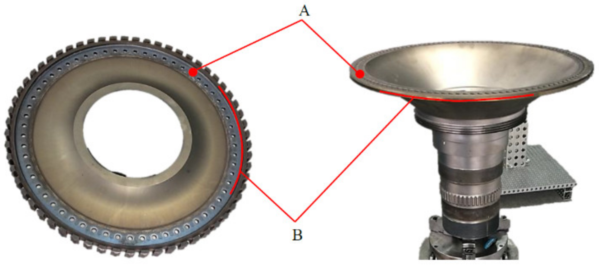
Figure 1 shows the matching form of the bayonet circular connector for the rotor components, which is mainly characterized by the combinatorial form of a planar pair and cylindrical pair. As can be seen from the figure, the contact pair between the adjacent parts contains a planar joint, such as the flange plane A, and a cylindrical joint, such as the locating spigot round B. Both constitute the partial parallel structure. Figure 2 extracts the key parts’ characteristics and gives certain tolerance requirements. Taking a two-stage rotor assembly as an example, the deterministic solution for the partial parallel dimensional chain is illustrated.
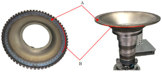
Figure 1.
The actual rotor parts. A: Flange plane. B: Locating spigot round.
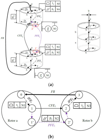
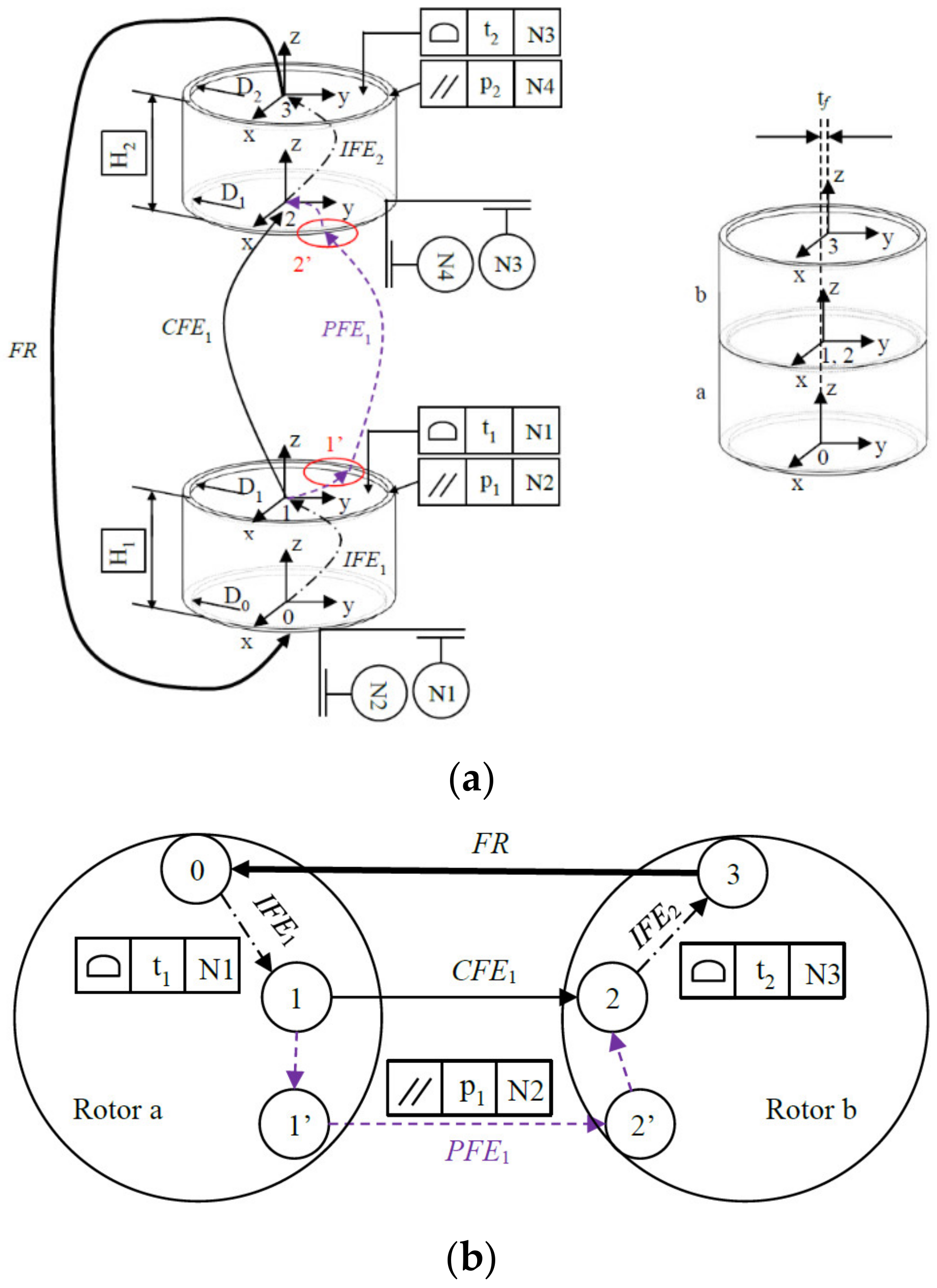
Figure 2.
Two-stage rotor assembly: (a) Assembly diagram; (b) Connection diagram.
As shown in Figure 2a, the global coordinate system 0, as well as three local coordinate systems 1, 2 and 3, are each built at the center of the related feature’s surface. The upper end face of each part contains one position variation (represented by a profile with a datum) and the upper cylindrical surface contains one direction variation (represented by a parallelism). Meanwhile, the lower end face and the lower cylindrical surface are determined as the assembly datum. In the global coordinate system, the accumulated concentricity variation (denoted by tf) of the upper end on part b is the functional requirement (denoted by FR), which needs to be controlled for the whole assembly.
According to the assembly diagram, the assembly connection relation of rotor a and rotor b can be determined. As shown in Figure 2b, the rotor assembly comprises a series main chain, namely IFE1-CFE1-IFE2-FR, and a partial parallel branch chain, namely CFE1-PFE1, wherein the position variations t1 and t2 are contained in the internal connection pairs (denoted by IFE1 and IFE2), and the direction variation p1 is contained in the contact connection pair (denoted by PFE1). The final FR is influenced by a combination of t1, t2, and p1.
2.2. Locating Principal Datum of Partial Parallel Chain
In the rotor stacking process, the upper end face and the locating spigot round of the lower part a serve as the datum reference of the upper part b, which provides an incomplete location path for rotor b. As a result, the upper rotor can rotate freely around the revolving axle. However, due to the existence of two constraint relationships for the partial parallel structure, two different positioning strategies need to be discriminated. As shown in Figure 1, one is a positioning strategy in which the planar pair marked with A is the primary positioning datum and the cylindrical pair marked with B is the secondary positioning datum. The other is a positioning strategy in which the cylindrical pair B is the primary positioning datum, and the planar pair A is the secondary positioning datum. In general, the influence of the positioning strategy on the variation propagation control and the datum robustness is greatly different because of the selection of the primary positioning datum.
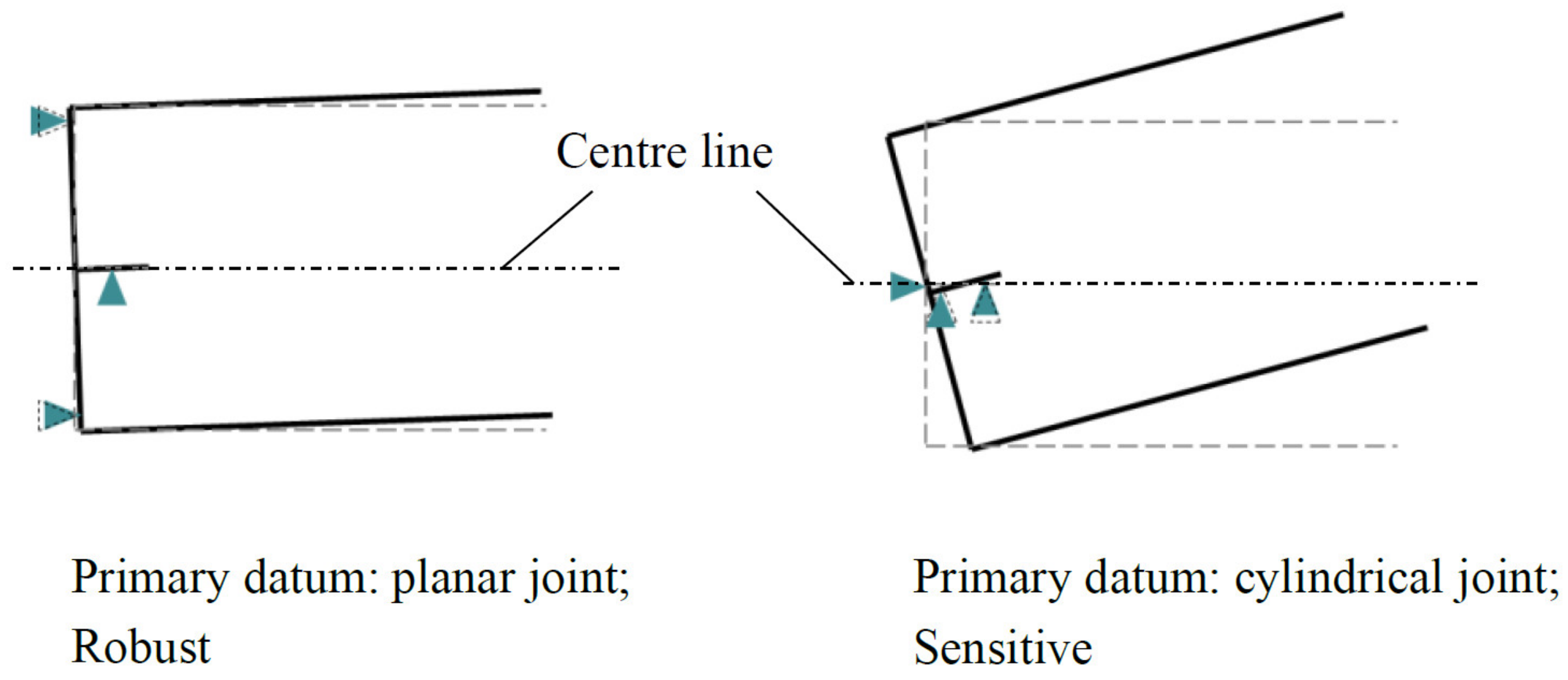
As shown in Figure 3, under different location paths, the primary positioning datum with the same amount of variation will cause different deflection degrees of the identical assembly. As can be seen from the figure, the planar pair is more robust to datum variations than the cylindrical pair. Therefore, choosing the upper end face as the primary positioning datum, instead of choosing the locating spigot round as the primary positioning datum, will be more conducive to the concentricity control of the rotor assembly. In fact, the fitting surface aera of the planar pair (see Figure 1A) is much larger than that of the cylindrical pair (see Figure 1B), and the former has a more significant effect on FR. Therefore, in the modeling process of rotor stacking, the planar pair is generally selected as the primary positioning datum. Reliable contact between the principal datums should be ensured first in the assembly process.
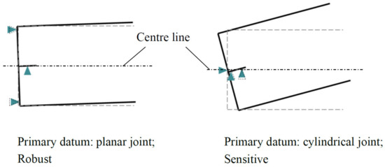
Figure 3.
Variation comparison under different positioning strategies.
Compared with assembly datum, there exists another type of datum, which is called part datum in this paper. The part datum is the characteristic element that is referred to in its internal tolerance design, such as the planar datum feature of N1 and the cylindrical datum feature of N2 in Figure 4. In this paper, to uniformly explain the model characteristics and analysis process, it is stipulated that the datum system, rotor structure, variation source type, and local coordinate system as shown in Figure 4 are adopted for each part-stage, to facilitate the subsequent three-dimensional variation modeling and analysis.
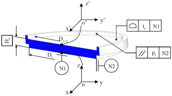
Figure 4.
The geometric model with variation information.
3. Unified Jacobian–Torsor Model and Its Improved Algorithm
3.1. J–T Model
Jacobian–Torsor (J–T) model consists of the Jacobian matrix and the torsor model. The assembly variation propagation is similar to the motion error propagation of a robot. As for the three-dimensional assembly dimension-chain, the relationship between each functional element (FE) and functional requirement (FR) can be expressed as follows:
where δs represents the variation translation on the X, Y, and Z axes of FR; δα represents the variation rotation around the X, Y, and Z axes; δqFEi represents the variation vector in the directions of six DOFs of the FEi; [J1 J2 J3 J4 J5 J6]FEi represents the 6 × 6 Jacobian matrix of the FEi.
As for the Jacobian matrix in Equation (1), its column vectors are:
On this basis, matrix variable [Win]3×3 is introduced:
where dxin = dxn-dxi, dyin = dyn-dyi, dzin = dzn-dzi, and n is the target point. Matrix (3) describes the position relation between the origin n of the coordinate system and the origin i of the coordinate system in Jacobian matrix [J].
Desrochers et al. [26] introduced a projection matrix [RPti] in consideration of the skew occurrence of the variation domain. [RPti] is a 3 × 3 matrix containing three groups of direction transformation vectors, which can effectively transform the variation direction of the variation domain into the variation analysis direction.
Based on the above analysis, the final Jacobian matrix is as follows:
Clément et al. [27] proposed the concept of technologically and topologically related surfaces (TTRS) based on Hervé’s [28] displacement set theory. According to its definition, the feature variation is described by vector sets, namely torsors. Since the feature variation is far less than the actual size of the assembly, the torsor is also called a small displacement torsor (SDT).
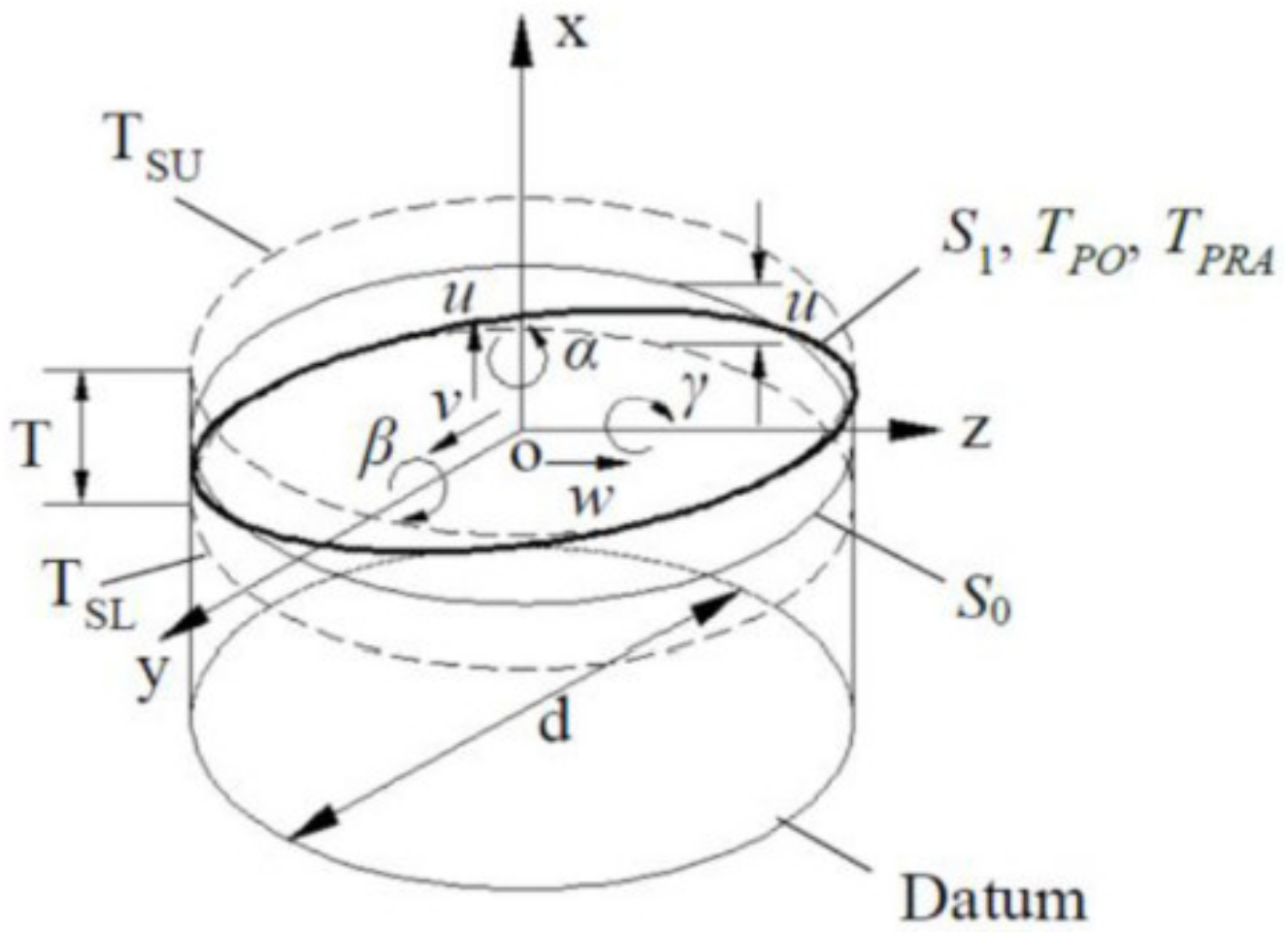
Generally, the SDT model involved six variational vectors: three motion vectors and three gyration vectors, which represent the position and direction of a function element, as shown in Figure 5.
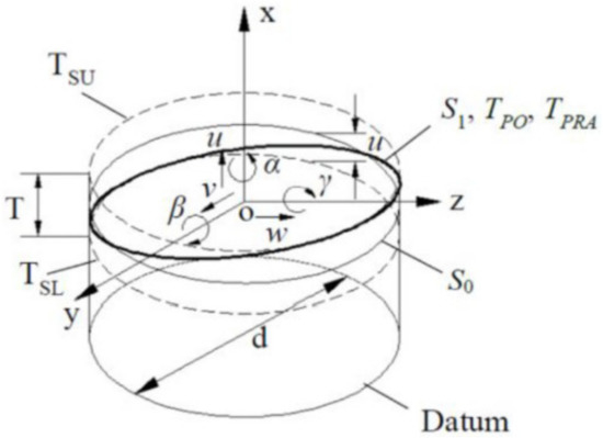
Figure 5.
SDT model.
Supposing that S0 is the nominal value of a characteristic, S1 is the arbitrary value of a variable surface, and the variation range of S1 relative to S0 is T, then the torsor S1 relative to S0 can be expressed as:
where u, v, and w are motion vectors along the X, Y, and Z axes in the local coordinate system, while α, β, and γ are gyration vectors around the X, Y, and Z axes.
SDT theory uses constraint and variation equations of the torsors to characterize the small changes of FE in the three-dimensional tolerance domain, and the Jacobian matrix uses matrix transformation to characterize the small displacements of point sets in an open-loop kinematic chain for rigid bodies. J–T theory combines the above two theories in the following form:
Expand Equation (6) to obtain:
where δui, δvi, δwi, δαi, δβi and δγi represent the actual variation components under self-constraint or motion constraint related to the i-th FE.
3.2. SDT Construction of Partial Parallel Structure
As shown in Figure 2b, this assembly contains a partial parallel structure consisting of mating feature CFE1 and PFE1. The CFE1 is composed of a planar joint that is regarded as the primary positioning datum, and the PFE1 is composed of a cylindrical joint that is regarded as the secondary positioning datum. The torsor of the part’s variation can be expressed as follows:
Equations (8) and (9) describe the existence and propagation form of the geometric variations at the connection position of the mounting surface. It is essentially a variation representation based on the surface variational method. However, this expression form results in interference between two SDT vectors, i.e., the gyration vectors of the planar pair (δα1, δβ1) are affected by the gyration vectors of the cylindrical pair (δα2, δβ2). To avoid such an interference, the smaller values between δα1 and δα2 as well as δβ1 and δβ2 need to be discriminated and screened, and then the effective vectors can be recombined before the subsequent calculation. However, the primary and secondary relations between positioning datums cannot be considered in this way, and it will be extremely complicated in the face of a large number of Boolean operations, such as intersection, union, etc., especially in multistage rotor assembly.
The other SDT expression can adopt the variation characterization method based on contact points under the incomplete positioning method. It is known that a completely free object is unconstrained in all six DOFs’ directions, while in actual assembly, a positioning constraint will eliminate all or part of its DOFs. For instance, in 3-2-1 deterministic positioning, the part will lose six DOFs in each direction, and its pose will be completely determined; similarly, in incomplete positioning, the part only loses the DOFs in some directions, and can also be adjusted by rotation or movement. The innovation of this paper is to regard the bayonet coupling structure of rotors as a united datums system, where the primary positioning datum restricts two rotational DOFs perpendicular to the principal axis of rotation, and one translational DOF parallel to the principal axis of rotation. Meanwhile, the secondary positioning datum restricts the remaining translational DOFs, ultimately preserving one rotational DOF around the principal axis, i.e., 3-2-0 incomplete positioning. It needs to be emphasized that the DOF analysis we have done assumes that the assembly is rigid. However, when the rotor system is flexible, the above analysis is no longer valid. This is because the pose position and orientation of the rotors are no longer uniquely determined. The deformation of the rotors will cause unpredictability in the results.
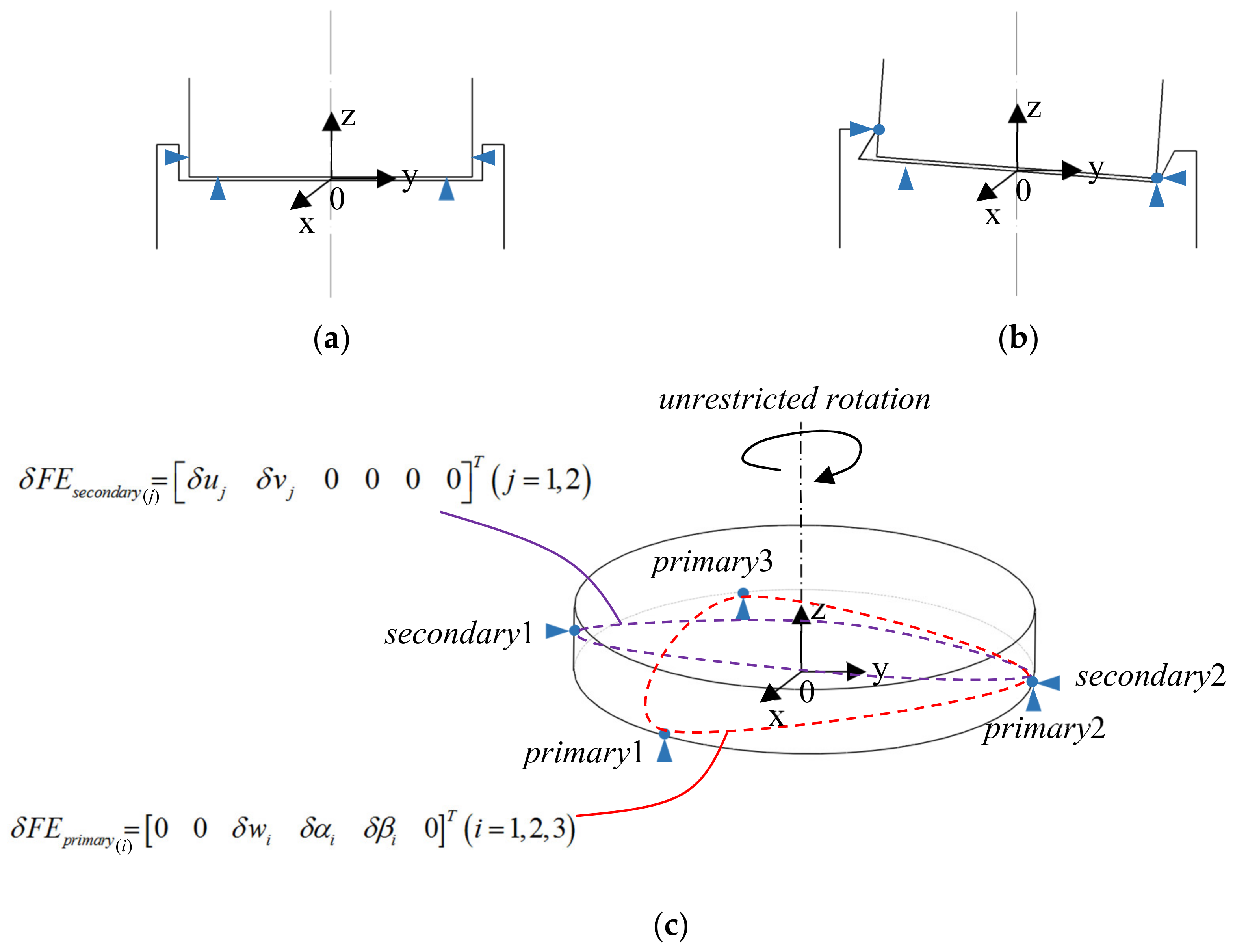
Ideally, the cylindrical pairs at the nominal value are generally regarded as the transition fit with the surface-to-surface contact. The contact points and analysis points are uncertain and can be selected arbitrarily, as shown in Figure 6a. However, the existence of variation will lead to an interference in the fit between the cylindrical pairs, where point-to- point contact appears. As a result, there is no relative movement between parts, as shown in Figure 6b. Of course, the deflection and translation of the parts must be within the tolerance limits. The contact points and analysis points follow the 3-2-0 positioning principle and can be uniquely determined by using precision measuring devices, as shown in Figure 6c.
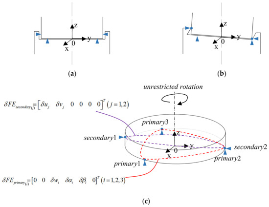
Figure 6.
Location method: (a) indeterminate location, (b) deterministic location, and (c) 3-2-0 positioning scheme.
Therefore, a variation matrix of the contact points has been derived. It is evident that whether the components of the matrix can be zeroed out depends on whether the DOFs of the corresponding components are zero.
Through this method, the tedious Boolean operation can be effectively avoided, and the computational efficiency can be greatly improved. Meanwhile, the influence of datum on assembly function and the effect of positioning order are considered, which provides feasibility for the following variation modeling and solving.
3.3. Contact Point-Based J–T Model Solution
This section will provide a detailed discussion of the expression of a partial parallel structure for aero-engine rotor assembly, and the solution method of partial parallel dimension chain of J–T model. According to Equation (10), the variation from the principal datum can be expressed as:
Likewise, the variation from the secondary positioning datum can be expressed as:
Therefore, the accumulated variation of the assembly involving m incomplete locating points can be expressed as:
where [δFRtotal]2 is the total rotor variation under the comprehensive influence of the locating points variations; δFRi represents the rotor variation due to the i-th locating point, including the primary datum points δFRprimary-part and the secondary datum points δFRsecondary-part; δFEprimary, δFEsecondary, and δFEpart represent the SDT variation of the primary datum points, secondary datum points, and rotor parts, respectively.
Based on the above analysis, the final expression of the total variation for the -stage rotor assembly can be derived as:
where all the parameters are the same as Equation (14).
Up to this point, the J–T equation considering multistage rotor assembly variations has been deduced. The equation has considered the united datum system of the parts and integrated the contact point-based SDT model and the Jacobian matrix of each functional element. In addition, the selection of contact points and analysis points conforms to the primary and secondary relationship of positioning datums.
3.4. Correction of Jacobian Matrix Considering Revolving Effect
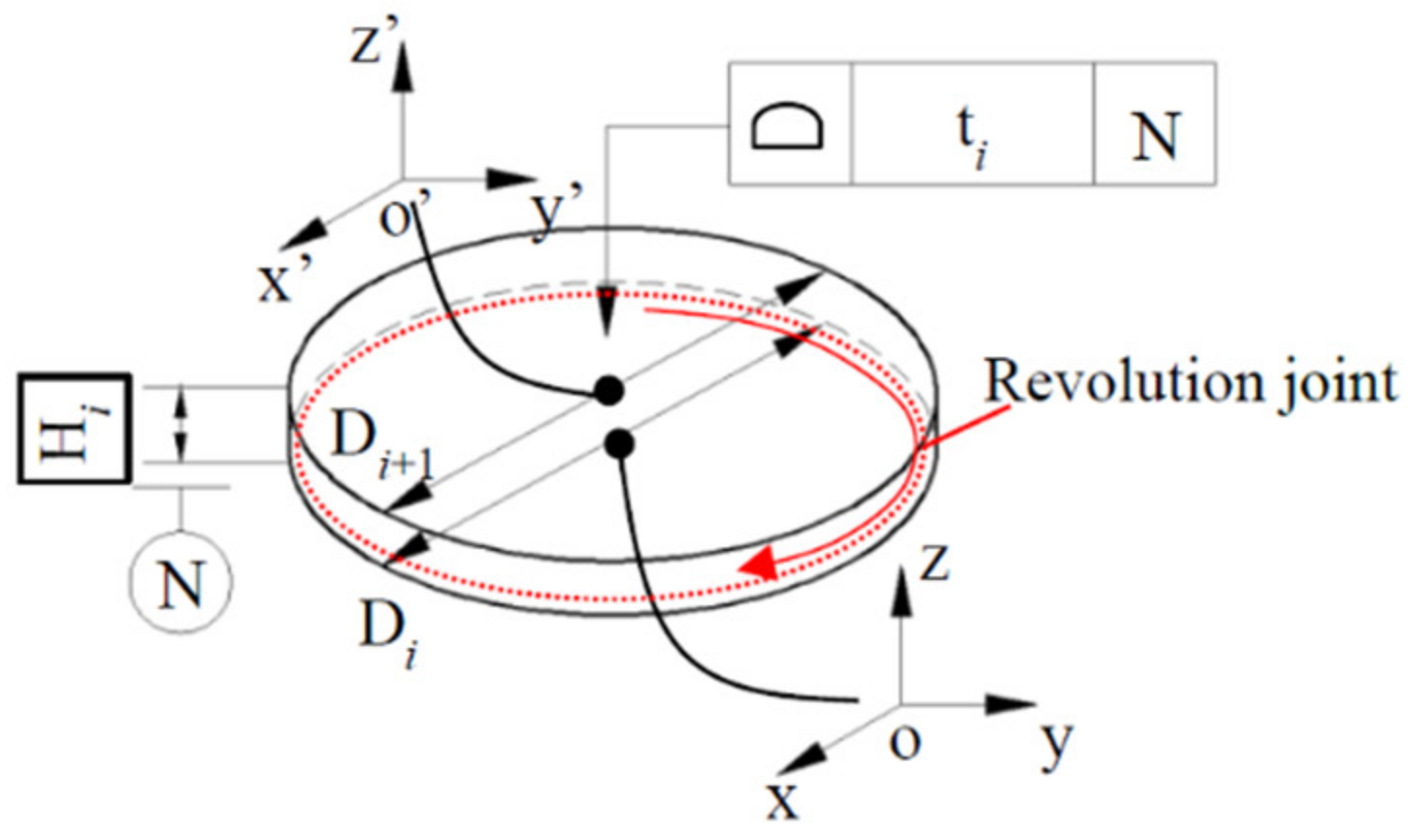
With a focus on the revolving characteristics of aero-engine rotors, the concept of the revolution joint (RJ) is introduced to characterize the rotating adjustment mechanism of the parts. As shown in Figure 7, the bottom surface of the revolving component is the part datum, and its top surface contains geometric tolerance. The RJ coincides with datum N and does not contain any tolerance information. It is evident that the RJ is essentially a contact functional element (CFE type), which can be easily expressed in a Jacobian matrix.
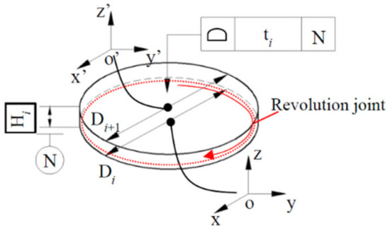
Figure 7.
Rotors with RJ.
For multistage rotor assembly, one contact type is composed of internal functional elements (IFE), and the other is composed of contact functional elements (CFE), namely the revolution joint (RJ). For the assembly of the revolving components, the highest concentricity can be obtained by rotating the parts to some appropriate angles around its axis of rotation.
There are, in total, n IFEs and (n−1) CFEs in an n-stage rotor assembly. The FRn is the top surface’s accumulative variations at the center of the local coordinate system n along the eccentric direction which is measured in the global coordinate system. Supposing that the i-th part is rotated θ(i−1) around the Z-axis, then in the global coordinate system, the general form of the locally oriented transformational matrix contained in the RJ can be expressed as:
In the n-stage revolving components assembly, the IFE mainly reflects the feature variation in the height direction, while the CFE mainly reflects the feature variation in the angular direction. By substituting matrix (16) into the matrix variable [Win] and matrix (4), the Jacobian matrix can be extended and modified in the direction of the part’s height and angle. The specific form of the extended Jacobian matrix [Je] containing the RJ is:
IFE:
CFE:
where Hi is the i-th component’s height; θi is the (i + 1)-th component’s installation angle relative to the global reference system.
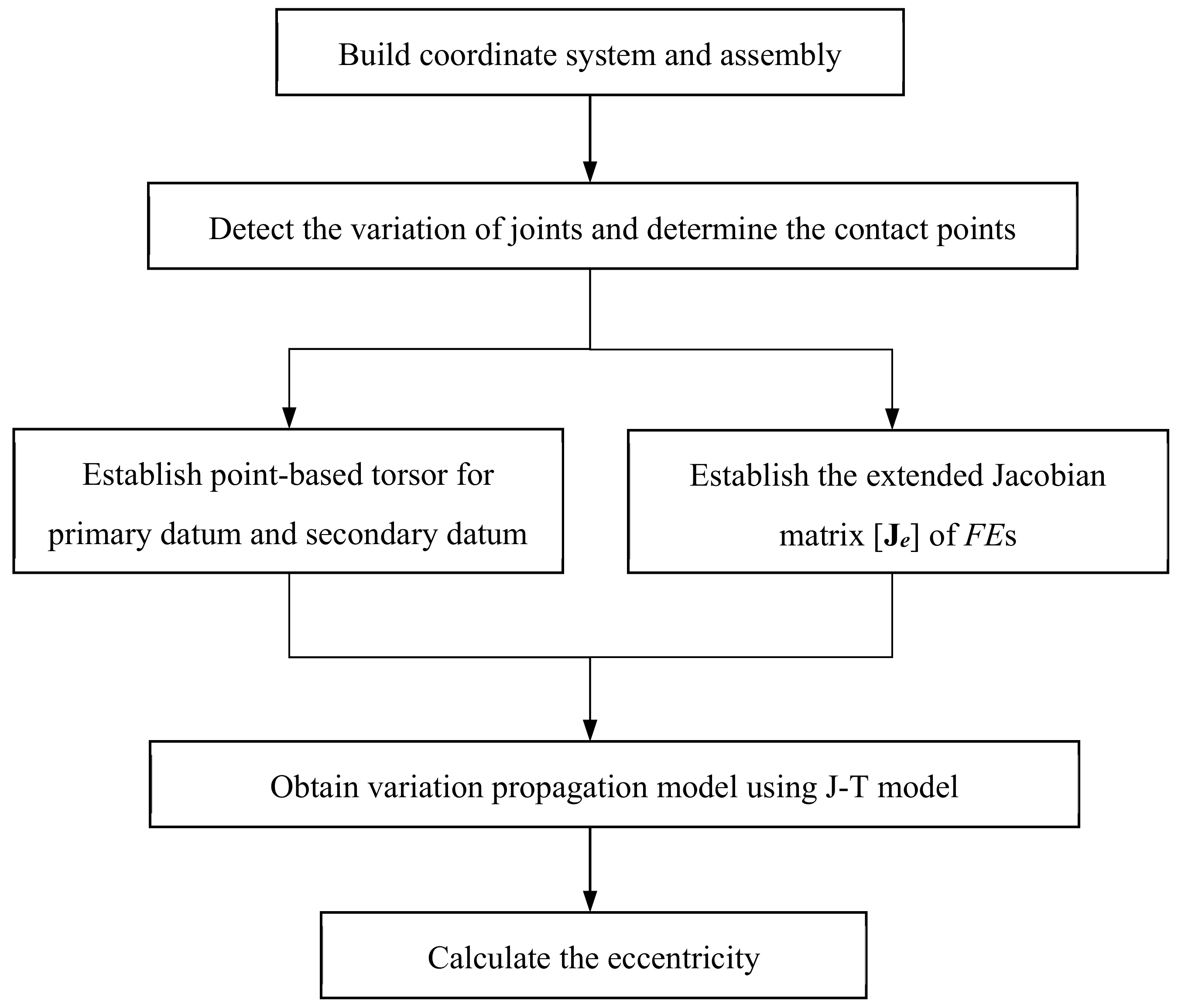
According to the Jacobian matrix characteristics, [[J1 J2 J3 J4 J5 J6]FE1…[J1 J2 J3 J4 J5 J6]FEn] represents the variation propagation process from FE1 to FEn. The modified Jacobian matrix [Je] can adequately reflect the parts’ revolving characteristics and the variation coupling effect between parts. On the basis of [[J1 J2 J3 J4 J5 J6]FE1…[J1 J2 J3 J4 J5 J6]FEn], the rotating adjustment process of each part-stage is further considered. The variation direction will change around the Z axis at the joint of two adjacent rotors, resulting in a change in the variation propagation path. The final variation propagation matrix becomes [[J1e J2e J3e J4e J5e J6e]FE1…[J1e J2e J3e J4e J5e J6e]FEn]. Figure 8 shows the overall calculation flow of the improved algorithm presented in Section 2.2, Section 3, Section 3.1, Section 3.2, Section 3.3 and Section 3.4. In the next section, the turbine rotor assembly will be taken as an example for detailed elaboration.
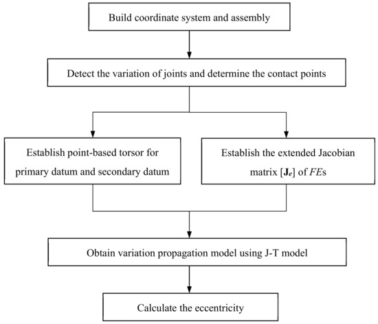
Figure 8.
Point-based solution of partial parallel chain model.
4. Case Study
4.1. Modeling and Solving
This section takes high-pressure turbine (HPT) rotor assembly as an example, to describe the variation expression and propagation of a partial parallel structure. The experimental program is tabulated in Table 2.
Table 2.
Experimental program.
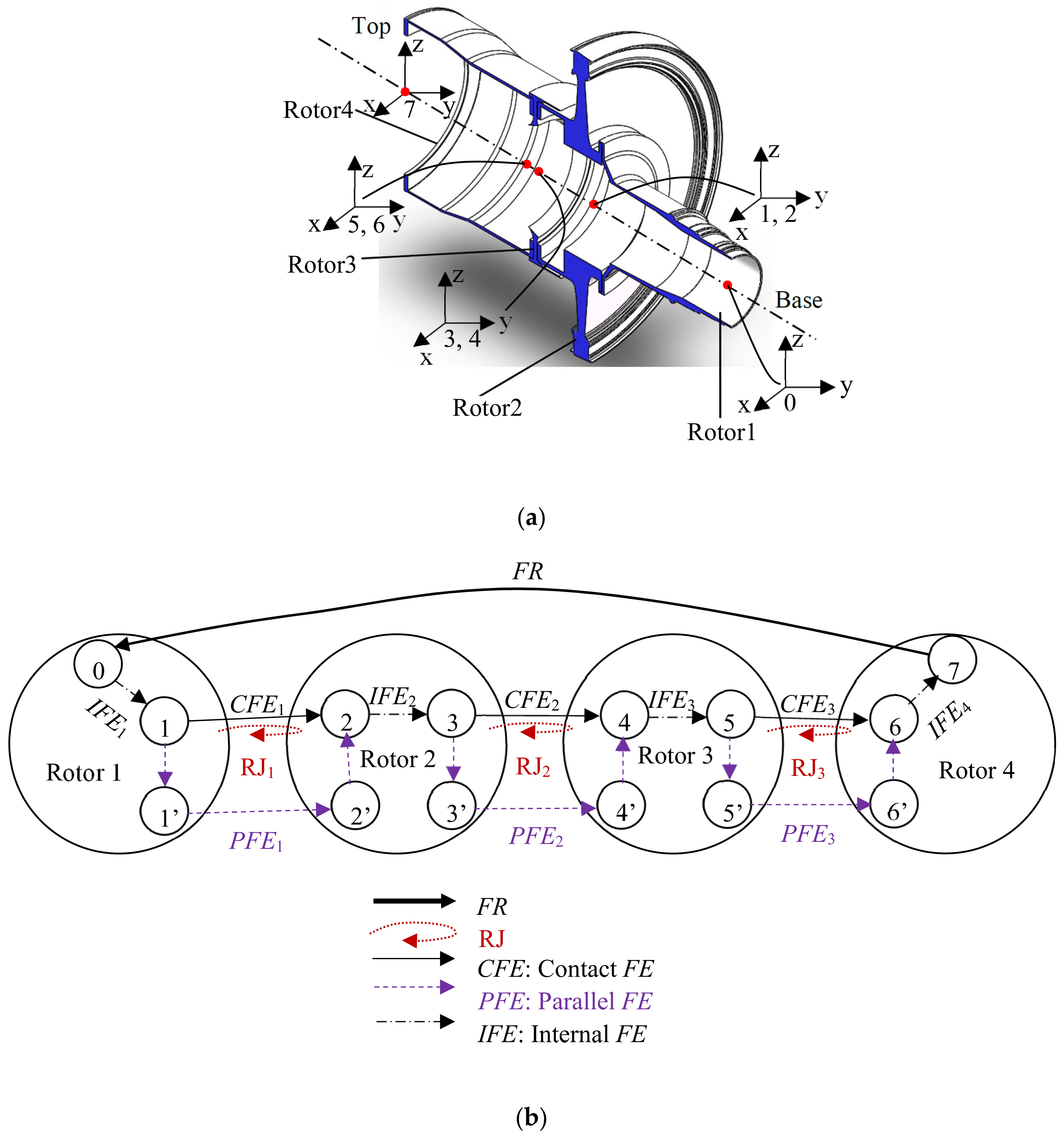
As shown in Figure 9a, the HPT sub-assembly is composed of four precision rotors, and each sub-coordinate system has been marked in the figure. The global coordinate system 0 is located at the datum center of the first-stage rotor, and the other local coordinate systems are located at the center of the relevant contact pairs. The assembly connection relation is shown in Figure 9b. It is evident that the main path for variation propagation is a series path: IFE1-CFE1-IFE2-CFE2-IFE3-CFE3-IFE4-FR, and there are also three partial parallel pairs: (CFE1-PFE1), (CFE2-PFE2), and (CFE3-PFE3). They also contain important variation information that affects the final FR.

Figure 9.
High-pressure turbine rotor assembly: (a) Parts drawing; (b) Connection diagram.
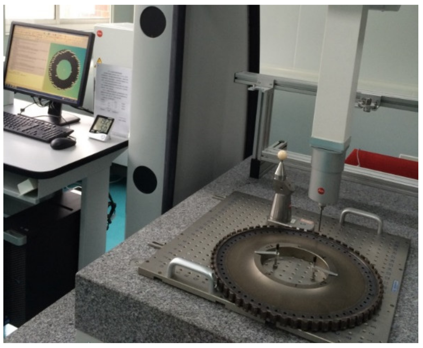
Table 3 lists the component’s dimensions and geometric tolerances which have been mentioned in Figure 4. Based on the point-based variation propagation algorithm proposed in the Figure 8, data on the feature surface of the parts should be firstly measured and collected. Figure 10 illustrated the process by using coordinate measuring machine of Leitz PMM-Xi to measure and collect the feature surface data. For every partial parallel pair, five analysis points including three primary-datum points and two secondary-datum points are designated. This process corresponds to step 1 in the Table 2. The specific variations of each point are listed in Table 4.
Table 3.
Dimensions and geometric tolerances of each component (Unit: mm).

Figure 10.
Measurement and data acquisition.
Table 4.
Jacobian matrixes and variation torsors of points for effective vectors.
According to the contact point variation listed in Table 4, the corresponding SDT can be obtained. It also lists the final variation torsor expression of the systematic points and the corresponding Jacobian matrix. Based on the assembly connection relation illustrated in Figure 9b and the Equation (15), the final variation accumulated function can be deduced as Equation (19):
where Hi is the i-th component’s height; Di is the i-th component’s cylinder diameter of its top end (i = 1, 2, 3, 4). The rest of the parameters are the same as shown in Table 4.
4.2. Results and Discussion
The above process is the key step for transforming a partial parallel chain into a series chain, in which the surface features are transformed into the point features. By substituting the Jacobian matrixes and variation torsors shown in Table 4 into Equation (19), the values of δutotal and δvtotal can be obtained, providing a basis for solving the following eccentricity. Finally, the accumulated results of the overall variations for four-stage rotor assembly are calculated as Equation (20) (Unit: mm for u, v, w; radian for α, β, γ):
where
Therefore, the eccentricity of the fourth-stage part can be calculated as follows (Unit: mm):
The accumulated eccentricity is 0.0539 mm, achieved by incorporating the partial parallel structures into the J–T model. Meanwhile, as can be seen from Equation (20), the accumulated rotational variations around the Z axis and each of the variation components are equal to zero, which means that all the variations involved in the calculation do not affect the rotational vectors of FR around the Z axis. Therefore, the operator can seek the best concentricity of the overall assembly by adjusting the orientation of each stage rotor around its axis of rotation. The above rules provide the basis and approach for the concentricity control of an aero-engine rotor assembly.
To validate the feasibility and accuracy of this method, traditional J–T models only considering the serial connections (IFE1- CFE1- IFE2- CFE2- IFE3- CFE3- IFE4- FR) are adopted for comparison. The results are as follows (Unit: mm for u, v, w; radian for α, β, γ):
As well, the eccentricity of the fourth rotor can be calculated as (Unit: mm):
As can be seen, without considering the influence of orientation variation, concentricity variation nearly increases more than threefold, from 0.0539 mm to 0.1595 mm, far exceeding the accuracy requirements (0.038 mm) of rotor assembly. In the actual assembly, the eccentricity variation of the fourth stage rotor is in the range of 0.030~0.040 mm. Apparently, the calculation results of the 3D variation model considering the partial parallel structure are more consistent with the practice.
On this basis, the concentricity variation control of the overall HPT rotors will be further discussed. According to the concrete form of the extended Jacobian matrix [Je] described in Equations (17) and (18), the extended Jacobian matrixes corresponding to the partial parallel pairs of all the stage rotors can be obtained, as shown in Table 5.
Table 5.
Extended Jacobian matrixes.
Replace the original matrix [J] in Equation (15) with [Je], and the assembly variation propagation function of a four-stage HPT rotor can be derived, which involves three RJs, as shown in Figure 9b and Equation (24):
where θi is the i-th (i = 2, 3, 4) component’s installation angle relative to the reference system 0. The subscript values start from two because the eccentricity calculation starts from the second component.
To measure the concentric performance of the whole assembly and consider the influence of the relationship between different parts’ variations, the multistage eccentricity index will be adopted as the overall evaluation index. Its specific expression is shown as Equation (25), and the corresponding governing equation is shown as Equation (26).
Multistage eccentricity:
Control target:
where εt is the multistage eccentricity; εi is the i-th component’s concentricity variation; ξi is the weighting coefficient of the i-th component’s eccentricity, indicating the importance of the i-th rotor part (i = 2, 3,…,n). This paper considers all parts to be of equal importance, and therefore ξi =1.
Combined with Equation (24), the eccentricity of the fourth stage rotor can be calculated as follows:
where
Similarly, [δutotal]i and [δvtotal]i can be calculated, and the eccentricity expression εi of the i-th rotor part can be obtained (i = 2, 3, 4). To optimize the overall concentricity of the HPT rotors, the multistage eccentricity εt needs to be controlled and optimized. According to Equations (25) and (26), the optimal θi needs to be found to minimize the εt. According to Equation (24), the target control equation of the four-stage HPT rotor stacking can be determined as follows:
For Equation (28), the genetic optimization algorithm is adopted. The following results are obtained: when the installation angles of the first stage, second stage, and third stage rotor are 3.153 rad, 6.025 rad, and 2.590 rad, respectively, the minimum value of multistage eccentricity εt can be worked out. Its value is 0.040 mm, close to the target control requirement of 0.038 mm.
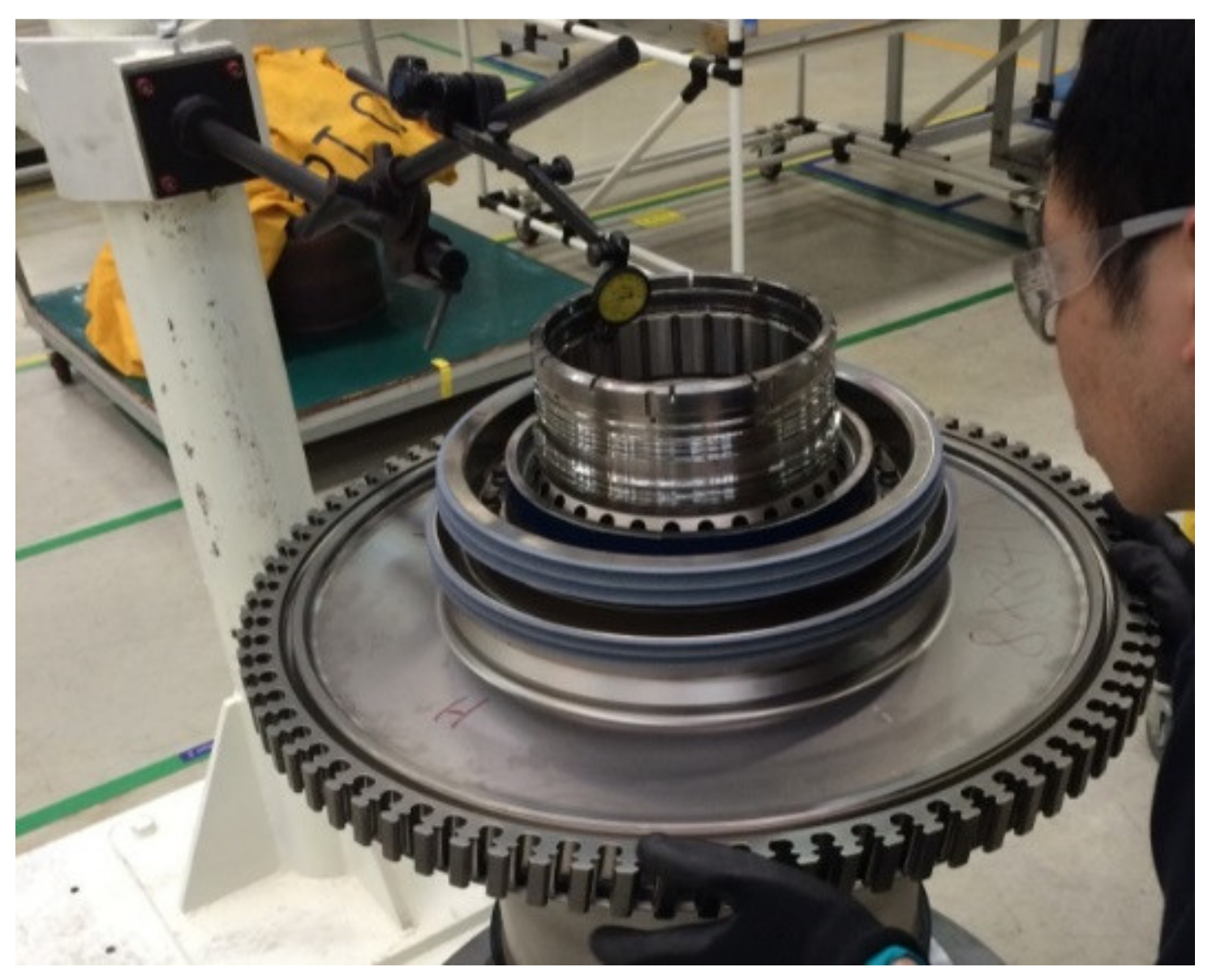
We used the calculated values to guide the actual installation, as shown in Figure 11. This process corresponds to steps 5 to 9 in the Table 2. It takes a total of 3 to 4 h to acquire a radial run-out of close to 0.038 mm. The optimal installation result is 0.037 mm.

Figure 11.
Adjustment and measurement of the experiment.
Comparing the calculated results with the best measured results, it is evident that the relative error is 8.1%. This is because the theoretical calculation model considers the parts as pure rigid bodies, ignoring the influence of contact deformation, interference compaction, morphology matching, and other factors. However, the theoretical calculation results still have high accuracy and guiding significance within the allowable error range. Under the guidance of θ2 = 3.153 rad, θ3 = 6.025 rad, and θ4 = 2.590 rad, the actual assembly results adequately meet the components concentricity requirements.
The comparative results showed that the proposed precision control method for rotor assembly based on an improved J–T theory adequately demonstrates the effects of a partial parallel structure. The proposed optimization method is beneficial to the variation propagation control of an aero-engine rotor assembly, which is highly practical. In recent years, there has been hardly any efficient computer-aided design (CAD) software to help workers reduce the workload in aero-engine assembly. It would take almost 4–5 days to finish the arduous task for two or three operators, and the use of only manual adjustments cannot satisfy the assembly precision requirements. The mathematical algorithm of this innovative precision control method could be integrated in CAD software to provide assistance to the operating personnel. With the aid of the proposed technique, the structural characteristics of rotors and geometric tolerance information could be adequately considered. The optimization results will contribute to guiding the actual rotor assembly and tolerance redesign.
5. Conclusions
This paper focuses on the characteristics of partial parallel connection for aero-engine rotor assembly and proposes a novel method for modeling and solving the partial parallel dimensional chain. By introducing the contact point-based SDT model into the traditional J–T theory and deriving the extended Jacobian matrix, a three-dimensional variation analysis model suitable for the connection characteristics of aero-engine rotors was constructed. The proposed method can apply not only to variation control of aero-engine rotor stacking, but also to assembly precision analyses of other revolving symmetric components. The following conclusions can be drawn:
(1) The innovation of this method is that by transforming the surface-to-surface contact model into a point-to-point model, the partial parallel dimensional chain is transformed into a series dimensional chain for the systematic points, which is easy to calculate. By considering the locating points as an independent assembly system, the function of the assembly variation expression in a general form is derived. The partial parallel dimension chain model can not only consider parts’ various geometric variations, but also allow for fixing the structure, a primary-secondary datum relationship, etc. It is beneficial to improve the prediction accuracy of the overall components.
(2) Combining aero-engine rotors’ structure and the assembly characteristics, the rotor’s variation propagation law was analyzed. By taking the partial parallel joints into consideration, the final concentricity variation was 0.0539 mm, which is far less than the 0.1595 mm of the traditional J–T model while only considering the serial chains, and much more closer to the true value range of 0.030–0.040 mm. The comparative results show that the point-based solution method for the partial parallel chain is more comprehensive and provides a theoretical basis for the analysis and control of assembly variations of the revolving components.
(3) The RJ was introduced to characterize the revolving characteristics of aero-engine rotors, and the extended Jacobian matrix was derived from this, which completes the second modification of the J–T model. Combined with the improved J–T model, a four-stage rotor assembly was adjusted. The highest concentricity of 0.040 mm can be obtained when the installation angles of each stage are 3.153 rad, 6.025 rad, and 2.590 rad. This outcome shows that this model can effectively predict the precision of the overall components and determine the best assembly scheme, which has strong practical guiding significance.
What needs to be pointed out is that it would be difficult to characterize the part’s deformation under actual working conditions. Thus, in the future, to model and optimize the actual assembly process for aero-engine rotors, the juxtaposition metamorphosis under the bolts’ load should be addressed, as well as the actual number of mounting angles, which depends on the number of bolts. Moreover, some machine learning methods can be adopted to achieve high computational efficiency, which can be conducive to guiding fulfillment of the assembly.
Author Contributions
Writing—original draft preparation, S.D.; writing—review and editing, S.D. and X.Z.; funding acquisition, S.D. All authors have read and agreed to the published version of the manuscript.
Funding
This work was funded by grants from the National Natural Science Foundation of China under Grant Number 52105509, and the Fundamental Research Funds for the Central Universities under Grant Number 2232019D3-33.
Acknowledgments
This work was financially supported by grants from the National Natural Science Foundation of China under Grant Number 52105509, and the Fundamental Research Funds for the Central Universities under Grant Number 2232019D3-33. The authors are grateful for this financial support.
Conflicts of Interest
The authors declare no conflict of interest.
References
- Cao, J. Status, challenges and perspectives of aero-engine simulation technology. J. Propuls. Technol. 2018, 39, 961–970. [Google Scholar]
- Zhang, H.; Li, X.; Jiang, L.; Yang, D.; Chen, Y. A review of misalignment of aero-engine rotor system. Acta Aeronaut. Astronaut. Sin. 2019, 40, 022717. [Google Scholar]
- Pan, G.; Chen, W.; Wang, M. A review of parallel kinematic mechanism technology for aircraft assembly. Acta Aeronaut. Astronaut. Sin. 2019, 40, 522572. [Google Scholar]
- Desrochers, A.; Clément, A. A dimensioning and tolerancing assistance model for CAD/CAM systems. Int. J. Adv. Manuf. Technol. 1994, 9, 352–361. [Google Scholar] [CrossRef]
- Zeng, W.; Rao, Y.; Wang, P.; Yi, W. A solution of worst-case tolerance analysis for partial parallel chains based on the Unified Jacobian-Torsor model. Precis. Eng. 2017, 47, 276–291. [Google Scholar] [CrossRef]
- Liu, J.; Sun, Q.; Cheng, H.; Liu, X.; Ding, X.; Liu, S.; Xiong, H. The state-of-the-art, connotation and developing trends of the products assembly technology. J. Mech. Eng. 2018, 54, 2–28. [Google Scholar] [CrossRef]
- Cao, Y.; Liu, T.; Yang, J. A comprehensive review of tolerance analysis models. Int. J. Adv. Manuf. Technol. 2018, 97, 3055–3085. [Google Scholar] [CrossRef]
- Chavanne, R.; Anselmetti, B. Functional tolerancing: Virtual material condition on complex junctions. Comput. Ind. 2012, 63, 210–221. [Google Scholar] [CrossRef]
- Chen, H.; Jin, S.; Li, Z.; Lai, X. A solution of partial parallel connections for the unified Jacobian–Torsor model. Mech. Mach. Theory 2015, 91, 39–49. [Google Scholar] [CrossRef]
- Li, W.; Zhu, N.; Shi, H.; Du, L. Study on the configuration of flexible assembly tooling for aero-engine discoid rotors. J. Shenyang Aerosp. Univ. 2013, 30, 6–9. [Google Scholar]
- Hong, J.; He, X.; Zhang, D.; Zhang, B.; Ma, Y. Vibration isolation design for periodically stiffened shells by the wave finite element method. J. Sound Vib. 2018, 419, 90–102. [Google Scholar] [CrossRef] [Green Version]
- Andersson, S. A study of tolerance impact on performance of a supersonic turbine. In Proceedings of the 43rd AIAA/ASME/SAE/ASEE Joint Propulsion Conference & Exhibit, Cincinnati, OH, USA, 8–11 July 2007. [Google Scholar]
- Forslund, A.; Söderberg, R.; Lööf, J.; Galvez, A.V. Virtual robustness evaluation of turbine structure assemblies using 3D scanner data. In Proceedings of the ASME 2011 International Mechanical Engineering Congress and Exposition, Denver, CO, USA, 11–17 November 2011. [Google Scholar]
- Liu, J.; Zhang, J.; Ding, X.; Shao, N. Integrating form errors and local surface deformations into tolerance analysis based on skin model shapes and a boundary element method. Comput. Aided Des. 2018, 104, 45–59. [Google Scholar] [CrossRef]
- Shi, J.; Liu, J.; Ding, X.; Yang, Z.; Gong, H. On the multi-scale contact behavior of metal rough surface based on deterministic model. J. Mech. Eng. 2017, 53, 111–120. [Google Scholar] [CrossRef]
- Sun, Q.; Huang, Q.; Sun, Z.; Qi, Y.; Sun, W. Interface parameter identification of bolted connections based on gradient virtual material. J. Mech. Eng. 2018, 54, 102–109. [Google Scholar] [CrossRef]
- Sun, Q.; Zhao, B.; Liu, X.; Mu, X.; Zhang, Y. Assembling deviation estimation based on the real mating status of assembly. Comput. Aided Des. 2019, 115, 244–255. [Google Scholar] [CrossRef]
- Wittwer, J.; Chase, K.; Howell, L. The direct linearization method applied to position error in kinematic linkages. Mech. Mach. Theory 2004, 39, 681–693. [Google Scholar] [CrossRef]
- Yang, Z.; Popov, A.; Mcwilliam, S. Variation propagation control in mechanical assembly of cylindrical components. J. Manuf. Syst. 2012, 31, 162–176. [Google Scholar] [CrossRef] [Green Version]
- Chen, H.; Lin, G.; Tang, T.; Yang, J.; Jin, S. A new approach of constraints establishment and optimization for matrix tolerance model. J. Mech. Eng. 2016, 52, 123–129. [Google Scholar] [CrossRef]
- Cai, W. A new tolerance modeling and analysis methodology through a two-step linearization with applications in automotive body assembly. J. Manuf. Syst. 2008, 27, 26–35. [Google Scholar] [CrossRef]
- Cao, Y.; Li, X.; Zhang, Z.; Shang, J. Dynamic prediction and compensation of aerocraft assembly variation based on state space model. Assem. Autom. 2015, 35, 183–189. [Google Scholar] [CrossRef]
- Zhang, W.; Chen, C.; Li, P.; Li, G.; Hu, J. Tolerance modeling in actual working condition based on Jacobian-Torsor theory. Comput. Integr. Manuf. Syst. 2011, 17, 77–83. [Google Scholar]
- Chen, Z.; Liu, Y.; Zhou, P.; Liu, G. Assembly tolerance analysis based on improved Taguchi method. Comput. Integr. Manuf. Syst. 2018, 24, 140–146. [Google Scholar]
- Pierce, R.; Rosen, D. A method for integrating form errors into geometric tolerance analysis. J. Mech. Des. 2008, 130, 467–478. [Google Scholar] [CrossRef]
- Desrochers, A.; Ghie, W.; Laperrière, L. Application of a unified Jacobian-Torsor model for tolerance analysis. J. Comput. Inf. Sci. Eng. 2003, 3, 2–14. [Google Scholar] [CrossRef]
- Clément, A.; Rivière, A.; Serré, P.; Valade, C. The TTRS: 13 constraints for dimensioning and tolerancing. In Geometric Design Tolerancing Theories, Standards and Applications; Springer: Berlin/Heidelberg, Germany, 1998. [Google Scholar]
- Hervé, J.M. Analyse structurelle des mécanismes par groupe des déplacements. Mech. Mach. Theory 1978, 13, 437–450. [Google Scholar] [CrossRef]

Publisher’s Note: MDPI stays neutral with regard to jurisdictional claims in published maps and institutional affiliations. |
© 2022 by the authors. Licensee MDPI, Basel, Switzerland. This article is an open access article distributed under the terms and conditions of the Creative Commons Attribution (CC BY) license (https://creativecommons.org/licenses/by/4.0/).