Simulation Analysis of Power Consumption and Mixing Time of Pseudoplastic Non-Newtonian Fluids with a Propeller Agitator

Abstract

In order to study the effect of a high twist rate propeller on the flow field characteristics of pseudoplastic non-Newtonian fluids, the numerical simulation method was used to analyze the mixing flow field of pseudoplastic non-Newtonian fluids at different concentrations in this paper. By changing the rotational speed and the blade installation height, the vorticity, turbulent energy, mixing power consumption, mixing time and mixing energy of the flow field were analyzed. By analyzing and comparing the research results, it was found that increasing the mixing propeller speed can effectively improve the mixing effect. Single-layer arrangement of mixing propeller is not suitable to be placed close to the bottom of the tank, and the mixing of the upper flow field is weaker. Under the same conditions, when the viscosity of pseudoplastic non-Newtonian fluid is increased, the high vorticity and high turbulence energy area is reduced to the mixing propeller area, and the time required for mixing 1.25% CMC solution is 246 times longer than that for mixing 0.62% CMC solution and the required mixing energy also increases sharply. The accuracy of the numerical simulation was verified by experiments. Considering the mixing effect and the mixing power consumption, the single-layer arrangement propeller is more suitable for mixing pseudoplastic non-Newtonian fluids with mass fraction of 0.62% CMC or below. This study can provide a reference for the practical application of propeller mixers to mix pseudoplastic non-Newtonian fluids.

1. Introduction

Pseudoplastic non-Newtonian fluids are widely used in the food and chemical industries. However, due to the special rheological properties of non-Newtonian fluids, they show different viscosity characteristics when mixing that make it more difficult to mix effectively, such as the generation of large dead zones, accumulation of stirring medium on the wall, higher mixing time, etc. Therefore, the requirements of the structural characteristics of the stirrer and mixing methods should be higher [1,2]. In industry, there are mainly two different types of agitation flow fields: radial agitator and axial agitator. The radial agitator can achieve a small range of mixing, but the entire stirrer can not be effectively mixed in a larger area. While the axial agitator can achieve a large range of mixing, compared with the radial agitator, the axial agitator has the advantages of large flow, low shear and high pumping [3]. The stirring method can be classified into gas stirring, liquid stirring and mechanical stirring. Mechanical stirring can effectively improve the consistency of the stirred medium and enhance the mass transfer process. According to the available literature, mechanical stirring is considered to be the most effective way under the same conditions of energy consumption [4].

In recent years, with the development of CFD technology, various turbulence models have been used to make calculations by researchers. The accuracy of the turbulence models is related to the prediction of the effectiveness in the mixing tank. Bakker [5] used the large eddy simulation method for the flow field in the stirred tank with different stirring paddles and found that the large eddy simulation can clearly obtain the non-stationary characteristics of the flow field. Haque [6] used four turbulence models: the k–ε model, the SST model and two differential Reynolds stress models (RST-LRR and RST-SSG) to analyze the accuracy of the flow field in the mixing tank. The accuracy of the results was consistent with the experiments. Wu [7] studied and analyzed the application of six turbulence models (Standard k–ε, RNG k–ε, Realizable k–ε, Standard k–ω, SST k–ω and Reynolds stress model) for stirring non-Newtonian fluids in anaerobic digestion reactions and the Realizable k–ε model was recommended.

In addition, mixing time and power consumption are two important analysis indicators in the mixing tank which affect the overall operating cost of the mixing tank. At present, we need the lowest mixing time and the lowest power consumption to achieve effective mixing. Li [8] used detached eddy simulation (DES) to simulate the local and global mixing time of a double standard six-blade Rushton turbine in the mixing tank. The feeding point has a large influence on the mixing process and mixing time, and the mixing efficiency is highest when the feeding point is located in the middle of the two impellers. However, this type of feeding is usually difficult to achieve, and, in most cases, the feeding is still carried out through the top of the mixing tank. Rosseburg [9] analyzed the mixing time by experimentally using the decolorization method, utilizing the fact that phenolphthalein is pink at pH above 8.2, and the mixing time was calculated by measuring the decolorization time of phenolphthalein after adding HCL by acid-base neutralization. Both numerical simulations and experiments can determine the mixing time [10,11,12,13], and numerical simulations are recommended when the mixing tank is large. Regarding the analysis of the power consumption of non-Newtonian fluids, researchers usually analyze torque on experiments and numerical simulations to measure power consumption and experiments are usually performed to verify the accuracy of numerical simulations [14,15,16,17,18,19]. For example, Cortada [20] used a mixture of glycerol and a gel formed of polyethylene glycol and Carbomer as the mixing medium to analyze the power consumption characteristics at different temperatures and mass fractions through experiments and numerical simulations, and the simulated torque values at low temperatures are closer to the experimental values.

The geometry and arrangement of the stirrer are also important factors that affect the effectiveness and efficiency of the mixing. In order to obtain the goal of adequate mixing, the researchers used different types of stirring impellers and arrangements for the analysis. Bao [21] used experiments to analyze the mixing performance of four different mixing impellers (a CBY or Pfaunder impeller as the inner one, and an anchor or helical ribbon HR as the outer one). These stirring impellers with different curvature have better mixing effect on the flow field but occupy a larger volume in the stirring tank. Houari [22] used CFD to analyze the effect of the Maxblend impeller on the operating conditions of shear-thinning fluid mixing. The structure of this stirring impeller is novel; however, the Maxblend impeller cannot generate enough circulation in deep laminar regime. For turbine type impellers, such as the Scaba 6SRGT, researchers have also conducted in-depth flow field research and analysis [23,24,25]. The design of various mixing systems has also been extensively studied, such as multiple shaft mixers, coaxial mixers, single and double central impellers, anchor combinations and eccentric shaft mixers [26,27,28,29]. The clearance of the impeller from the bottom of the tank also has a significant effect on fluid mixing. Rutherord [30] found that mixing was best when the distance from the bottom of the impeller-specific tank was one-third of the entire height of the mixing tank. Argang [31] used a coaxial mixing system composed of two central impellers and an anchor to analyze the effect of different clearances on mixing, and the most suitable configuration was found when the impeller pitch was almost equal to the impeller diameter and 0.185 m from the bottom of the tank.

In order to study the type of propeller in the mixing tank. Yoshihito [32] et al., used a propeller with a variable pitch impeller (similar to pitched paddle impellers) to analyze the power consumption characteristics and obtained satisfactory results. Zhong [33] studied the solid–liquid mixing performance of the propeller, it was found that the shear moment is smaller, so it is suitable for high-speed rotation, and could obtain the stirring effect of large flow and strong circulation with low energy consumption. Wang [34] designed a side-entry propeller and conducted an experimental study of shear-thinning fluids by using an ultrasonic Doppler anemometer (UDA). Viscous and axial forces jointly affect the separation effect of the flow, and the shear-thinning behavior of the fluid was enhanced due to the tangential flow generated by the viscous force.

CMC solution is a typical pseudoplastic non-Newtonian fluid with obvious shear-thinning characteristics. Because pseudoplastic non-Newtonian fluids in food and chemical industries are mostly opaque and turbid solutions, CMC’s aqueous solution is transparent, non-toxic and odorless and has good light transmission, so it is widely used in flow field research by researchers [35,36,37]. Romano [38] used 3D particle tracking velocimetry (3D-PTV) to measure and analyze the flow field characteristics during the stirring of the CMC solution. When Re < 400, the rheological property of non-Newtonian fluid significantly reduces the ability of impeller to pump the surrounding fluid. Low fluid circulation has a negative effect on macroscopic mixing. High speed ensures a large flow of fluid in the mixing tank, but the power consumption associated with high speed is too high for industrial purpose.

An extensive literature review suggests that little information is available regarding the mixing with high twist rate propellers, and, to the best of the authors’ knowledge, no papers have been published on this type of mixer for shear-thinning fluids. A detailed understanding of the mixing characteristics of propeller blades with high twist rates is still needed. Therefore, the purpose of this paper is to investigate the flow characteristics of pseudoplastic non-Newtonian fluids at different concentrations and speeds by numerical simulations with a three-twisted-blade propeller as the mixer. In order to ensure the reliability of the numerical simulation calculations, an independently designed experimental platform was used for verification. The mixing time and power consumption characteristics of CMC solutions with different mass fractions were compared and analyzed. Our research can deepen the understanding of non-Newtonian fluids with high twist propellers and provide a reference for the practical design and application of propeller mixers.

2. Mixing System and Experimental Setup

The mixing system under study (Figure 1a) is a cylindrical unbaffled tank with a flat bottom (diameter D = 400 mm and height H = 490 mm), equipped with a propeller with three twisted blades (diameter d/D = 0.6, height h/H = 0.1), and the cylindrical shaft at the blades joint is set to 0.16. Two types of clearance to the mixing tank base are designed here (s₁/H = 0.06, s₂/H = 0.18). The ratio d_s/D (diameter shaft) is set to 0.05, and the 3D diagram of the mixing impeller is shown in Figure 1b.

The experiments were conducted by using an independently designed experimental platform, as shown in Figure 2. Where 1—variable frequency motor; 2—torque meter (error range ±2 rpm and ±0.001 N·m); 3 and 4—reactor cover plate; 5—air bearings (reduces errors caused by shaft friction) and 6—shaft.

3. Theoretical Background

Three mass concentrations of CMC solutions were used in this study ($\omega$₁ = 0.62%, $\omega$₂ = 0.85%, $\omega$₃ = 1.25%). In this paper, CMC solution with medium concentration and high concentration was selected to effectively derive the working status that can be achieved by a single layer propeller. Rheological experiments were performed with Anton Paar ViscoQC-300 at a constant temperature of 25 °C to determine the rheological properties of the three solutions. After experimental measurement and nonlinear fitting, these three mass fractions of CMC solutions had a shear-thinning behavior modeled by the power-law [39]. In this case, the constitutive equation and the viscosity equation are as follows:

$$\tau =K·{\dot{\gamma }}^n$$

(1)

$$\eta =K·{\dot{\gamma }}^{n-1}$$

(2)

where $\tau$ is the shear stress, $\dot{\gamma }$ is the shear rate, and K and n are the consistency index and the flow behavior index, respectively.

The numerical values of consistency index and flow behavior index are shown in

Table 1. Rheological property of the stirring medium.

Stirring Medium	$\mathit{K}/\left(\mathbf{P}\mathbf{a}\mathbf{·}{\mathbf{s}}^{\mathbf{n}}\right)$	n	${\mathit{\eta }}_{\mathbf{m}\mathbf{i}\mathbf{n}}/\left(\mathbf{P}\mathbf{a}\mathbf{·}\mathbf{s}\right)$	${\mathit{\eta }}_{\mathbf{m}\mathbf{a}\mathbf{x}}/\left(\mathbf{P}\mathbf{a}\mathbf{·}\mathbf{s}\right)$	$\mathit{\rho }/\left(\mathbf{k}\mathbf{g}\mathbf{·}{\mathbf{m}}^3\right)$
0.62% CMC	1.75	0.464	0.02	0.79	1004
0.85% CMC	4.99	0.388	0.03	2.87	1005
1.25% CMC	15.34	0.325	0.14	11.98	1010

, and the rheological properties of CMC solutions are shown in Figure 2. As can be seen from Table 1, when the viscosity of the solution increases, the consistency index of the fluid increases and the fluid flow behavior index decreases. The shear stress increases with the increasing shear rate, and the apparent viscosity decreases with the increasing shear rate, which can be clearly seen in Figure 3.

The state of fluid can be judged by the Reynolds number. For Newtonian fluids, the Reynolds number is defined as follows:

$$Re=\frac{\rho N{D}^2}{\eta }$$

(3)

The dynamic viscosity of the non-Newtonian fluid is related to the shear rate. In this paper, a classical calculation method proposed by Metzner and Otto [40] in 1955 is used to assume that the average shear rate in the stirrer is related to the stirrer speed as follows:

$${\gamma }_{avg}={\kappa }_{s}N$$

(4)

where ${\kappa }_s$ is the Metzner constant. This assumption is based on the laminar flow throughout the stirrer but has been widely used in transitional and turbulent flow states recently [41]. According to [42], ${\kappa }_s$ takes 11.5. Therefore, the generalized Reynolds number equation used in this paper is as follows:

$$R{e}_M=\frac{\rho N^{2-n}{D}^2}{K{\kappa }_s^{n-1}}$$

(5)

where $\rho$ is the density and N is the propeller rotational speed. The Reynolds number of flows at different rotational speeds is shown in

Table 2. Reynolds number of flow at different speeds.

Stirring Medium	$\mathit{R}{\mathit{e}}_{\mathit{M}}$
	N = 60	N = 90	N = 120	N = 150	N = 180	N = 210	N = 300	N = 600
0.62% CMC	61.4	114.4	178.04	250.82	331.89	420.55	727.35	2109.25
0.85% CMC	25.95	49.88	79.32	113.66	152.49	195.50	347.42	1061.97
1.25% CMC	9.89	19.51	31.52	45.91	62.31	80.66	146.60	468.13

.

The power consumption is an important parameter to describe the performance of a mixing system. It can be calculated by integrating the viscous dissipation in all the vessel volumes:

$$P=\eta \int Q_{v}dv$$

(6)

where $Q_v$ is the viscous dissipation.

The power number is calculated as:

$$N_p=\frac{P}{\rho N^3{D}^5}$$

(7)

4. Numerical Method

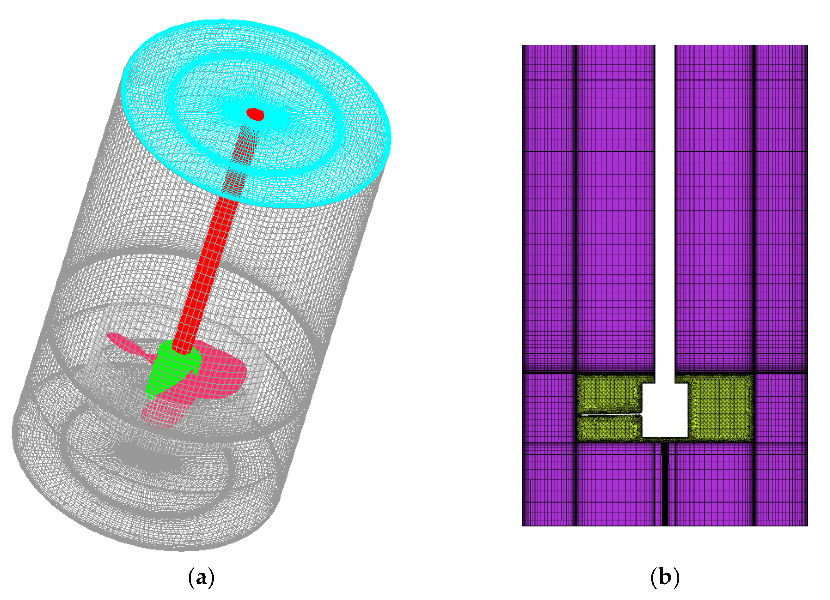
The physical model was built using UG/NX and meshed using CFD pre-processing software ICEM. The fluid domain is divided into rotation zone and stationary zone, each of which uses various reference systems to transfer data between the zones through interfaces.

In this paper, the commercial software Fluent 18.0 was used. The multiple reference system (MRF) method was used to calculate the steady state of the rotating model of the agitator. This method has been used by several scholars to mix the same system and satisfactory results have been obtained [43]. The solution of the flow field was based on the pressure–velocity solver, and the SIMPLE algorithm was adopted, which has a good convergence and fast calculation speed. For transient calculations, the results of the steady-state calculations were used as the initial flow field, and the rotational model of the stirrer used the sliding mesh method (SMM), and the velocity–pressure coupling was carried out by the PISO algorithm. On the top of the tank surface, the symmetry boundary conditions were applied. The propeller surface was set as a zero-shear stress boundary and no-slip boundary condition was set at the bottom of the mixing tank and the cylindrical wall [44]. The main convergence criterion for each solution was that the normalized residuals of physical variables, such as power number and velocities, reach a steady state. This means that it does not change significantly with further increases in time steps or number of iterations. The scaled residuals of all conservation equations were obtained when the residuals were less than 10⁻⁶ [45].

The Realizable k–ε model was used as the turbulence model in this work. Realizable k–ε turbulence model is widely used for rotating shear flow and pipe flow. The reason to use a turbulence model rather than laminar is that, with the exception of highly viscous fluids mixed at a low impeller speed, mixing in the tanks always creates turbulence [46].

The stirring propeller in the mixing tank has a complex structure and has curved blades. Therefore, the overall mesh was divided using a combination of hexahedral and tetrahedral meshes. The tetrahedral mesh was chosen to provide more stable grids and to reduce the number of low quality cells. Because the mesh density in the computational grid needs to be fine enough to capture the flow details, the grid near the tank walls and rotating propeller were encrypted. For the same number of grids, the unencrypted grid can only converge to 10⁻⁴ in numerical simulation, and the encrypted grids can converge to 10⁻⁶.

Grid independence was verified by comparing power criterion of different mesh quantities. As can be seen from

Table 3. Mesh independence check.

Mesh Size	${\mathit{N}}_{\mathit{p}}$
2,690,565	0.918
3,673,721	0.949
5,603,586	0.956

, when the number of grids exceeds 3,673,721, the power number only changes 0.7% with the increase of the number of grids, which can be considered to have reached the requirement of grid-independent convergence solution, where the number of grids in the rotating domain is 1,844,201 and in the stationary domain is 1,829,520 (Figure 4).

5. Results and Discussion

5.1. Validation of the Numerical Results

First, it is necessary to verify the accuracy of the numerical calculation method. The power consumption obtained from the experimental measurements was analyzed and compared with the numerically calculated at s₁/H = 0.06.

The solutions with mass fractions of $\omega$₁ = 0.62%, $\omega$₂ = 0.85% and $\omega$₃ = 1.25% CM were used as experimental media. The Re and N_p were calculated by measuring the stirring propeller torque at 70 sets of speeds in the range of 6–168 r/min and the results were compared with the numerical simulation values.

The numerical simulation has four calculation points of 60 r/min, 90 r/min, 120 r/min and 150 r/min, respectively, under each mass fraction, for a total of twelve calculation points. The 0.62% CMC solution has a high power criterion when the Reynolds number less than 100. The numerical results are in good agreement with the experimental values. They have the same trend of variation and prove that the adopted turbulence model is desirable (Figure 5). The next part of this paper will use this calculation method for analysis.

5.2. Effect of Rotation Speed and Clearance

Figure 6 shows the streamline and velocity distribution of the flow field at 120 rpm, 150 rpm, 180 rpm, 210 rpm, 300 rpm and s₂/H = 0.18. The rotating propeller produces an axial jet in the impeller area, and the maximum velocity appears at the blade tip, so the flow field near the blade tip is relatively intense. When the rotating speed increases, the CMC solution appears as the shear-thinning phenomenon, which changes the viscosity of the fluid, thus changing the flow pattern of the flow field. The mainstream circulation area of the flow field increases, while the reverse flow circulation area decreases, which leads to a wider range of fluid flow. The center of the entire mainstream circulation area is basically in the center plane of the propeller. When the blades disturb the rotation of the fluid, the rotating fluid is divided into two reverse circulation flow and two reverse circulation areas appear at the lower end of the paddle and near the liquid surface, which enhances the convection between the fluid. Due to the three-blade arrangement of the propeller, the vortex is asymmetrically distributed in a plane.

To sum up, with the increase of Reynolds number, the main circulation area increases, the reverse circulation area decreases, the convection between fluids increases, and the velocity gradient increases, which drives a wider range of fluid flows. Therefore, increasing the rotating speed can effectively improve the stirring effect of non-Newtonian fluid.

The horizontal surface velocity distribution of different Reynolds numbers at the section Z = 110 shows (Figure 7) that the high velocity area is concentrated at the tip of the propeller, with the increase of Reynolds number, the area of the high velocity increases. When N = 300 rpm, the area of high velocity reaches the maximum. The rotating speed has a great influence on the horizontal velocity. With the increase of the rotating speed, the horizontal velocity increases.

Figure 8 is the streamline velocity diagram of the plumb cross section with s₁/H = 0.06 and long axis arrangement. This arrangement has a strong disturbance at the bottom. Compared with the s₂/H = 0.18 arrangement, the impeller is closer to the bottom, the rotating fluid can directly impact the bottom of the tank, and there is almost no reverse circulation flow area at the bottom, but the mixing is weaker in the upper area of the mixing tank.

It can be seen that with the increase of velocity, the main flow circulation area increases, the reverse flow circulation area decreases, the convection between the fluids increases and the velocity gradient increases, which drives a larger range of fluid flow.

In addition, the maximum axial velocity in the mixing tank is used as the denominator to calculate the axial velocity and analyze the time-average velocity distribution, and the dimensionless axial velocity was expressed as ${\nu }^{*}$. The trend of the axial velocity distribution of s₁/H = 0.06 (Figure 9) and s₂/H = 0.18 (Figure 10) arrangement of the vertical section is the same. With the increase of rotating speed, the axial velocity changes dramatically. The axial velocity of s₂/H = 0.18 is changed from negative to positive and then back to negative. The positive velocity appears in the effective stirring area of the propeller, the maximum positive axial velocity appears near Z = 90 mm, and the maximum negative axial velocity appears at Z = 140 mm. In this interval for the impeller height, the existence of negative velocity indicates the existence of circulation, and the positive and negative change of axial velocity is exactly for the trend of the cloud chart, and there are three circulation zones. The axial velocity in the s₁/H = 0.06 arrangement, the axial velocity changes from positive to negative, the maximum positive axial velocity appears at Z = 30 mm, the maximum negative axial velocity appears at Z = 80 mm, and the axial velocity only changes from positive to negative, which indicates that the effective disturbance area of the propeller with s₁/H = 0.06 arrangement includes the bottom of the tank. When the propeller is closer to the bottom of the stirrer, the diversion phenomenon no longer occurs, corresponding to the cloud diagram only exists in two circulating flow areas.

In this paper, the maximum radial velocity in the mixing tank is used as the denominator to dimension the radial velocity, and the dimensionless radial velocity is expressed as $u^{*}$. Figure 11 shows that the dimensionless radial velocity of the horizontal section is asymmetrically distributed on the horizontal plane at the central axes of s₂/H = 0.18, Z = 60 mm, Z = 110 mm and Z = 160 mm, and the radial velocity distribution in the three horizontal sections are similar. Because the propeller adopts a three-blade arrangement, the radial velocity is asymmetrically distributed in the horizontal plane, and the radial velocity direction is opposite. The radial velocity increases first along the diameter direction, the extreme value appears at the tip of the propeller and then gradually decreases due to viscous drag. The radial velocity shows an opposite distribution along the symmetry axis because the fluid in the mixing tank flows circumferentially along the mixing axis. The radial velocity distribution is highest at Z = 110 mm. The second highest radial velocity distribution is at Z = 160 mm, and both higher radial velocities appear at Z = 160 mm cross section nearer to the stirring shaft. When the stirring shaft rotates, the stirring shaft disturbs the fluid in a small area near the stirring shaft, resulting in a relatively high radial velocity. Z = 60 mm has the lowest radial velocity distribution, and Z = 60 mm is in the lower region of the stirring paddle, where mixing is weak.

5.3. Effect of Fluid Rheology

To investigate the effect of the rheological properties of non-Newtonian fluids (CMC) on the stirred flow field, CMC solutions with mass fractions of $\omega$₁ = 0.62%, $\omega$₂ = 0.85%, $\omega$₃ = 1.25% and s₂/H = 0.18 and N = 300 rpm were selected.

From the vertical cross-sectional streamline and velocity distribution diagram (Figure 12), it can be seen that the overall structure of the flow field is similar. When the mixing fluid is a $\omega$₁ = 0.62% CMC solution, there is no reverse flow circulation area, which is very beneficial to fluid mixing. As the mass fraction of CMC solution increases, the fluid viscosity increases, the main stream circulation area decreases and the reverse flow circulation area increases, which weakens the convection flow between fluids and reduces the overall flow velocity of the stirring field, which increases the stagnant area in the stirring tank and is not conducive to mixing.

In order to analyze the effect of non-Newtonian fluid rheological properties on the velocity field of the horizontal section, the variation law is analyzed at the Z = 110 mm (Figure 13) section. The area of the high velocity zone is similar, but with the increase of viscosity, the area of the high velocity zone decreases in the direction away from the diameter. Shear-thinning only takes place in the area attached to the stirring paddle and cannot cause disturbance to the fluid further away, therefore reducing the stirring effect. The rheological properties of non-Newtonian fluids are more obvious, when stirring the viscosity of the fluid, the speed should be increased to increase the shear rate of non-Newtonian fluids and increase the degree of fluid mixing in the mixing tank. From the axial velocity distribution of the vertical cross section (Figure 14), it can be seen that the axial velocity changes the most when the stirred fluid is $\omega$₁ = 0.62% CMC solution, and there is still a flow rate near the liquid surface, which indicates that the stirring effect is better at this concentration. However, as the mass fraction of CMC solution increases, the viscosity increases and the axial velocity decreases. Especially when mixing $\omega$₃ = 1.25% CMC solution, the maximum axial speed is only half of $\omega$₁ = 0.62% CMC at the given speed. The viscosity of the fluid has a great impact on the stirring effect, and when stirring a high viscosity fluid, the speed needs to be increased to enhance the mixing efficiency.

Vortex is a unique form of fluid flow; from boundary layer flow and mixed flow to turbulent flow, the structure of these flows are vortices. Vorticity is used to describe the intensity and direction of the vortex. The intensity is the rotational degree of the fluid velocity vector, and the direction is the same as the direction of the angular velocity and is defined as follows:

$$\overrightarrow{\Omega }=2\overrightarrow{\omega }$$

(8)

where $\overrightarrow{\Omega }$ is the vorticity and $\overrightarrow{\omega }$ is the angular velocity.

The vorticity distribution of the flow field can directly reflect the flow of the field. The vorticity distribution in the vertical section shows (Figure 15) that the maximum vorticity appears at the tip of the propeller blades and the vortex area extending outward. The vorticity distribution area of $\omega$₁ = 0.62% CMC solution is the largest, and the high vorticity area shrinks toward the center of the stirring propeller as the CMC concentration increases, especially when stirring $\omega$₃ = 1.25% CMC solution, the high vorticity area is only distributed in the effective mixing area of the mixing propeller, and the mixing effect is weaker.

Turbulence is caused due to the existence and development of vortices, and the turbulent pulsation is caused because the continuous mixing of fluids. Turbulent kinetic energy is an important variable to characterize the intensity of the velocity pulsation, which is closely related to the microscopic mixing of the liquid [47] and is defined as follows:

$$k=0.5\left(\overline{u^{\prime 2}}+\overline{v^{\prime 2}}+\overline{w^{\prime 2}}\right)$$

(9)

where u’, v’ and w’ are the values of pulsation velocity in the radial, axial and circumferential directions and k is the turbulence kinetic energy.

The distribution of turbulent kinetic energy in the vertical section shows (Figure 16) that the red color is the high turbulent kinetic energy zone, the maximum value of turbulent kinetic energy appears at the top and the bottom of the propeller, and a small part of the high turbulent kinetic energy zone exists at the top of the propeller. As the fluid viscosity increases, the overall high turbulent kinetic energy zone of the stirred tank flow field decreases, and the high turbulent kinetic energy zone of the lower part of the propeller gradually shrinks to the inside.

The turbulent kinetic energy is further elaborated by Y = 90 mm plumb line data graph, and the turbulent kinetic energy is nondimensionalized with the squared value of the blade tip velocity V_tip as the denominator. It can be seen from the figure (Figure 17) that the distribution of the turbulent kinetic energy is similar as a whole, with the first wave peak appearing at the tip of the propeller blade and the second wave peak appearing in the upper region of the blade, and the highest turbulent kinetic energy occurs at a mass fraction of $\omega$₂ = 0.85% CMC, and its distribution also corresponds to the cloud map. When the concentration is 0.62%, the rotating speed of 300 rpm can effectively stir the fluid, and the turbulent kinetic energy in the stirring tank is more widely distributed. As the mass fraction of CMC solution increases, the high turbulent energy area shrinks to the blade area, and the viscosity change is not obvious in the upper area of the stirred tank.

5.4. Power Consumption

The following image (Figure 18) shows the curve of power criterion with a generalized Reynolds number under different concentrations and shaft lengths. It can be seen that the non-Newtonian fluid with different concentrations has the same changing trend. Comparing the power consumption characteristics of s₂/H = 0.18 under the same Reynolds number, the 0.62% CMC solution has a higher power criterion: that is, when stirring a low mass fraction CMC solution, the required power consumption is lower. Comparing with the mass fraction of 0.85% CMC, the power consumption required for the long axis is higher when Re is less than 100, and there is almost no difference in power consumption when Re is greater than 100.

5.5. Mixing Time

The time required in the mixer for the material to reach the required degree of mixing is called the mixing time [48]. Mixing time is an important indicator of the mixing degree of reaction materials. In Fluent, by using the Species Transpor model, materials with the same physical properties are only physically mixed without chemical reaction. The volume of one-fifth of the cylinder in the mixing tank was set as the tracer, and the initial concentration of the material inside the cylinder was set to 100% in Patch and 0% outside. During the transient calculation, the tracer concentration in the stirred tank changes as a whole, and the overall concentration was 20% after complete mixing. By setting the monitoring points in the mixing tank, the specific location is shown in Figure 19. Inside the tracer meter, there are 10 monitoring points on the upper part, the side part and the bottom of the stirring paddle. When the monitoring point concentration reaches the specified concentration, the mixing is completed, and the time used is the mixing time.

With the mixing process, the material concentration approaches to 20%. At this time, the arrival time is recorded as t₉₅ (95% mixing principle), and when the material concentration reaches 19–21% the mixing is completed. From Figure 20a it can be seen that at the beginning of stirring Point2 has a faster decrease in tracer concentration compared to Point1, and the concentration of material in Point7 increases faster than that in Point6. Compared with Point1 and Point6, the vortex generated by mixing has a more obvious effect on these two points. As can be seen from Figure 20b, the material concentration of Point10 is the lowest to reach the specified degree, and this point is located directly under the stirring paddle. In this area, the propeller in the mixing process cannot be effectively turned, so the material can only be mixed through the interaction between the surrounding fluid when the stirring paddle causes them to flow.

Mixing energy is a comprehensive indicator reflecting the degree of mixing, Considering the impact of mixing power and mixing time, the greater mixing energy usually means the lower the mixing efficiency. The mixing energy calculation formula is as follows:

$$Q=P\times t_{95}$$

(10)

where Q is the mixed energy.

The power number, mixing time and mixing energy for CMC solutions with mass fractions of $\omega$₁ = 0.62%, $\omega$₂ = 0.85% and $\omega$₃ = 1.25% at N = 600 rpm and s₁/H = 0.06 and s₂/H = 0.18 are given in

Table 4. Computed parameters through mixing time simulation at N = 600 r/min, s₂/H = 0.18.

Stirring Medium	${\mathit{N}}_{\mathit{p}}$	${\mathit{t}}_{95}/\mathbf{min}$	$\mathit{Q}/\mathbf{k}\mathbf{J}$
0.62% CMC	0.621	0.098	0.516
0.85% CMC	0.637	0.898	4.874
1.25% CMC	0.697	24.182	143.604

and

Table 5. Computed parameters through mixing time simulation at N = 600 r/min, s₁/H = 0.06.

Stirring Medium	${\mathit{N}}_{\mathit{p}}$	${\mathit{t}}_{95}/\mathbf{min}$	$\mathit{Q}/\mathbf{k}\mathbf{J}$
0.62% CMC	0.646	0.309	1.701
0.85% CMC	0.652	9.486	52.658
1.25% CMC	0.693	170.881	1008.314

, respectively.

As can be seen from Table 4, as the concentration of the mixture increases, the time required for homogeneous mixing rises sharply. When the mass fraction reaches 1.25%, the time and the power consumption required for homogeneous mixing is about 1000 times longer than that under 0.62% mass fraction, which results in low mixing efficiency. By comparing Table 4 and Table 5, the required mixing uniformity time and the power consumption for s₁/H = 0.06 are several times larger compared to the s₂/H = 0.18 arrangement. Therefore, when mixing high-viscosity non-Newtonian fluid, it is not suggested to use a single propeller near the bottom. In general industry, due to the limitation of motor and propeller technology, the speed of propeller can not reach a higher speed. If the experimenter wants to mix higher viscosity fluid, they can increase the diameter of the propeller and adopt the multi-layer arrangement of mixing propeller.

6. Conclusions

In this paper, the flow characteristics of CMC solutions with mass fractions of 0.62%, 0.85% and 1.25% at different rotational speeds and different arrangement heights of the propeller were compared, and the main conclusions were obtained as follows.

With the increase of mixing propeller speed, the shear rate of fluid increases, the viscosity of non-Newtonian fluid decreases, the main stream circulation area expands and the reverse flow circulation area decreases, which intensifies the convection between the fluids, and the overall flow velocity of the mixing field increases. Increasing the speed is conducive to the mixing of fluids in the tank.

Comparing the height of propeller arrangement, s₁/H = 0.06 can effectively mix the bottom area of the mixing tank, but the mixing effect on the upper layer of the mixing tank is weak, and s₂/H = 0.18 has a better mixing effect on the whole. The single-layer arrangement of the propeller is not suitable for placement close to the bottom of the mixing tank.

When the mass fraction of the CMC solution is 0.62%, 0.85% and 1.25%, respectively, increasing the solution viscosity changes the rheological characteristics of non-Newtonian fluids obviously. The main circulating flow region is reduced, the reverse circulating flow region is expanded, the convection between fluids is weakened and high the vorticity and high turbulence kinetic energy zone narrows towards the mixing propeller area. Therefore, the high viscosity CMC solution is not conducive to homogeneous mixing, and the speed should be increased appropriately to promote the mixing of fluids in the mixing tank.

Under the same operating conditions, the time required for homogeneous mixing increased sharply with the increase of the mass fraction of CMC solution. When mixing 0.62% CMC solution, the time required to mix uniformly was only 0.098 min, while when the mass fraction reaches 1.25% CMC solution, the time required to mix uniformly increased 246 times and the required stirring power consumption had already exceeded its income, so the single-layer arrangement of stirring propeller could not mix it effectively. From this it can be concluded that the single layer propeller is suitable for mixing CMC solutions with mass fractions of 0.62% or below.