Lithium Battery State-of-Charge Estimation Based on a Bayesian Optimization Bidirectional Long Short-Term Memory Neural Network

Abstract

State of charge (SOC) is the most important parameter in battery management systems (BMSs), but since the SOC is not a directly measurable state quantity, it is particularly important to use advanced strategies for accurate SOC estimation. In this paper, we first propose a bidirectional long short-term memory (BiLSTM) neural network, which enhances the comprehensiveness of information by acquiring both forward and reverse battery information compared to the general one-way recurrent neural network (RNN). Then, the parameters of this network are optimized by introducing a Bayesian optimization algorithm to match the data characteristics of lithium batteries with the network topology. Finally, two sets of lithium battery public data sets are used to carry out experiments under different constant temperature and variable temperature environments. The experimental results show that the proposed model can effectively fit the actual measurement curve. Compared with traditional long short-term memory network (LSTM) and BiLSTM models, the prediction accuracy of the Bayes-BiLSTM model is the best, with a root mean square error (RMSE) within 1%, achieving a better ability for capturing long-term dependencies. Overall, the model exhibits high accuracy, adaptability, and generalization for the SOC estimation of batteries with different chemical compositions.

1. Introduction

With the increasing severity of the global energy crisis and the environmental pollution caused by transportation energy consumption, the world’s demand for efficient and clean energy is also increasing year by year. As a type of reusable, rechargeable battery, lithium batteries greatly reduce carbon emissions and chemical fuel consumption. In addition, due to the advantages of high energy density, low self-discharge rate, and long service life, lithium batteries are widely used in electric vehicles [1,2]. As one of the most important state quantities of lithium batteries, the SOC is not only an important parameter for measuring the remaining power of batteries but also an important index for ensuring the safety and service life of batteries [3]. Therefore, accurate lithium battery SOC estimation is currently a key problem to be solved.

The SOC is defined as the ratio of the remaining capacity to the nominal capacity of a battery [4], which is usually calculated by Equation (1). It should be noted that SOC is a state quantity that cannot be measured directly, and there are highly nonlinear relationships between the SOC and observable variables, such as voltage, current, temperature, and other measured data. Using these observable variables, the SOC value can be obtained indirectly. However, these variables also change with battery aging, ambient temperature, and driving conditions, which makes accurate SOC estimation a challenge [5].

$$\mathrm{SOC}=\frac{Q_c}{Q_i}\times 100\%$$

(1)

where $Q_c$ is the current remaining capacity of the battery and $Q_i$ is the nominal capacity of the battery. The SOC value range is between [0,1]. When the SOC is 0, the battery is completely discharged. When the SOC is 1, the battery is fully charged.

At present, there are four main types of SOC estimation methods proposed by scholars: the ampere-hour integration method, the open-circuit voltage method, the model-based estimation method, and the data-driven method [6]. The ampere-hour integration method mainly involves calculating the amount of electricity released by the battery over a period of time by measuring the discharge current of the battery and integrating the current over time, thus achieving battery SOC estimation [7]. The open-circuit voltage method is mainly used to find the relationship between the open-circuit voltage (OCV) and the battery SOC, and a corresponding OCV–SOC table is established by using discharge experiments to further estimate the SOC according to the mapping relationship between them. The model-based method characterizes the internal characteristics of the battery by establishing a battery model to establish a time-domain space state equation to estimate the SOC [8,9,10]. However, due to high computational complexity, the model’s requirement for prior knowledge, and the variations of a large number of parameters in the model with operating conditions, it is difficult to accurately estimate the SOC of the battery throughout its life cycle using the model-based method. In recent years, the data-driven approach has received much attention from scholars because it does not require a specific battery model and an accurate formula. The data-driven approach treats the battery as a black box and only requires the lithium battery measurement signal to achieve the estimation of SOC [11]. Many scholars have used many traditional machine learning methods to simulate the nonlinear characteristics of batteries, which have suitable data integrity, and the relationships between the battery SOC and the observable variables (voltage, charge/discharge current, resistance, etc.) can be learned autonomously from the data. Common learning algorithms include support vector machines, semi-supervised learning, artificial neural networks, etc. [12,13]. Reference [14] uses a multi-hidden layer backpropagation (BP) neural network to learn the nonlinear relationship between battery SOC and Li-ion battery measurable variables (i.e., current, voltage, and temperature). Using a genetic algorithm to denoise the prediction error, this method successfully captures the long-term dependence between the observable variables and the battery SOC. Reference [15] uses the least-squares support vector machine (LS–SVM) model to train the dynamic characteristics of lithium-ion batteries with a small sample and realize the online application of the modeling method. However, these shallow learning architectures lack comprehensiveness when considering the redundancy of feature information, which ultimately leads to low accuracy.

In particular, with the booming development of artificial neural networks, deep learning is also widely used for battery SOC estimation. Deep learning, as an important branch of machine learning, can easily capture the relationships between the measured signals and the SOC by building multilayer deep neural networks with nonlinear transformations to extract feature information from input samples. RNN is a deep learning method based on neural networks, which has been favored by many scholars in recent years in regard to the prediction problem of sequence data. Reference [16] proposed an SOC estimation method based on RNN by using the time-series memory capability of RNN. Through the data obtained from the lithium battery performance test experiment, a battery SOC estimation simulation experiment was carried out under high-power discharge conditions. Reference [17] proposed an SOC estimation model combining RNN with the Coulomb counting method. The model takes voltage, current, and temperature as inputs and considers the effect of battery degradation during charging and discharging to estimate battery SOC under three different operating conditions. However, the structure of RNN is relatively shallow, and a typical RNN is unable to learn the intrinsic features of the measured data layer by layer upon encountering the extended sequence problem. To improve the capability of RNNs in handling sequential data, an LSTM, gated recurrent unit (GRU) structure can be added to RNN to solve the vanishing gradient phenomenon problem. Reference [18] proposed a method to accurately estimate lithium battery SOC by using LSTM and formed a single network that correctly estimated the SOC under different ambient temperature conditions by encoding the time-dependent term. Reference [19] estimated lithium-ion battery SOC based on a gated recurrent neural network (GRU-RNN) and established mapping relationships between the battery observable variables and SOC to achieve battery SOC estimation at different temperatures. In the literature [2], a gated recurrent neural network model with an activation functional layer (GRU-ATL) was proposed to estimate the battery charge state, and a stable and accurate SOC estimation performance was achieved by estimating the battery SOC online under different operating conditions without relying on the battery model. Reference [1] proposed a method combining a denoising auto-encoder (DAE) with a GRU to estimate lithium battery SOC. By reducing noise and increasing the dimension of battery measurement data to obtain useful data information and then using GRU-RNN for training, experimental results were obtained that showed that the proposed DAE-GRU had suitable robustness. All of these studies achieved suitable results for battery SOC estimation, but most of these studies only focus on the correlation of forward series data, while the correlation study of reverse series data acquisition is lacking. Reference [20] proposed an SOC estimation method combining multichannel convolution and bidirectional recurrent neural network (MCNN-BRNN) to sequentially estimate SOC by extracting multi-scale local robust features and using the BRNN to capture effective time-varying signals. This reduced the accumulation of errors and improved the overall estimation accuracy. Reference [21] proposed a stacked bidirectional long short-term memory (SBLSTM) model for estimating lithium battery SOC. This method captured the forward and reverse battery information through the bidirectional structure and improved the depth of the model by stacking the bidirectional structure, which further improved the estimation performance of the model. It is worth mentioning that the network setting of the model in this document is highly random. Artificially setting the super parameters of the network will not only increase the training cost of the model but also affect the prediction effect of the model. Therefore, the parameter adjustment of the model needs to be further resolved. In this paper, a Bayesian optimization-based bidirectional long short-term memory (Bayes-BiLSTM) neural network model is proposed for lithium battery SOC estimation. Compared with the unidirectional LSTM network, this model uses a bidirectional structure to summarize the temporal dependence of past and future contexts by capturing the forward and reverse battery information. In addition, compared with other methods, the proposed model also introduces a Bayesian optimization algorithm. The introduction of this optimization algorithm assists in finding the optimal network parameters to improve the network performance and compensates for the defect of manually setting the network parameters. In particular, this paper adopts the Bayesian optimization algorithm to optimize the parameters of the BiLSTM model. The optimization parameters include the number of hidden layer neurons $I_s$, the maximum number of iterations MaxEpochs, the initial learning rate $I_r$ and the learning decline rate factor $I_{rdf}$. Finally, this paper evaluates the effectiveness and applicability of the proposed method by conducting multiple sets of comparative experiments using two public lithium battery data sets, and the experimental results show that under different constant temperature and variable temperature environments, the proposed method has better accuracy, adaptability, and generalizability for the SOC estimation of different types of lithium batteries.

The rest of the paper is organized as follows: the second part details the LSTM, BiLSTM, and Bayes-BiLSTM models. The third part introduces the lithium battery data set and experimental procedure. The fourth part analyzes and discusses the experimental results. The fifth part comprises the conclusion of this paper.

2. SOC Estimation Methods

2.1. LSTM Network

The models of traditional neural networks will only focus on the processing of information in the current moment and will not infer whether the processing of information in the previous moment will help in the next moment, and the problems of local minima, gradient disappearance, and gradient explosion are prevalent when performing model training. For example, the gradient disappearance generated by RNN during backpropagation can lead to the inability to capture long-term dependence [17]. LSTM networks effectively solve this problem. LSTM is a special implementation of RNN, which improves the implicit layer and introduces the concept of temporal order on top of RNN neural networks so that the output of one moment can have a direct impact on the input of the next moment.

The structure of the LSTM hidden unit is shown in Figure 1, which includes a forgetting gate $f_t$, an input gate $i_t$, an output gate $o_t,$ and a memory cell $C_t$. The sigmoid layer determines which values need to be updated, and the tanh layer determines what new values to add. The transfer and control of information is achieved through three gates. The forgetting gate $f_t$ in the cell state transfer determines what information should be discarded. The input gate $i_t$ controls the decision of what new information to add to the “cell state”. The output gate $o_t$ controls the storing of the information of the cell at the moment t to the hidden state of $h_t$ [21,22]; that is, the output is obtained. Equations (2)–(5) demonstrate the execution process of updating the internal unit by LSTM.

$$f_t=\sigma \left(w_{fx}{x}_t+w_{fh}{h}_{t-1}+b_f\right)$$

(2)

$$i_t=\sigma \left(w_{ix}{x}_t+w_{ih}{h}_{t-1}+b_i\right)$$

(3)

$$o_t=\sigma \left(w_{ox}{x}_t+w_{oh}{h}_{t-1}+b_o\right)$$

(4)

$$s_t=tanh\left(w_{cx}{x}_t+w_{ch}{h}_{t-1}+b_c\right)$$

(5)

where w and b with subscripts represent the weight matrices and deviation vectors of the three gates; $\sigma (\cdots )$ is a sigmoid activation function with a function value of a vector between (0,1) that acts as a gate, with 0 representing discard and 1 representing retention; $tanh(\cdots )$ normalizes the values to between (−1,1) and is used to update the internal cells and cell outputs, and $s_t$ is a vector of candidate values created after the tanh layer.

In the whole information flow, the process of cell state from $C_{t-1}$ to $C_t$ is similar to a conveyor belt, and the cell update rule from $C_{t-1}$ to $C_t$ is as follows:

(a)

Select the part of old cell information forgotten through the “forgetting gate”, multiply the old state with $f_t$, and discard the information determined to be discarded.

(b)

Add the candidate cell information $s_t$ through the “input gate” and then add $i_t\times s_t$ to obtain the cell state $C_t$ as in Equation (6).

$$C_t=f_t{C}_{t-1}+i_t{s}_t$$

(6)

The output of the LSTM cell is calculated by Equation (7):

$$h_t=o_{t}tanh\left(C_t\right)$$

(7)

2.2. Bidirectional LSTM Network

LSTM improves the gradient disappearance or explosion problem that occurs in traditional RNNs due to its complex gated memory mechanism and outperforms other recurrent architectures in dealing with sequential tasks with long-term dependencies. However, it is worth noting that the LSTM structure can only use positive dependencies, and some useful information will be filtered in the long-term gated memory chain. To solve this problem, this paper adopts a bidirectional LSTM, which consists of two LSTM layers in different directions, two independent LSTM layers, one for inputting the forward sequence and the other for inputting the reverse sequence. The structure of the BiLSTM is shown in Figure 2. This structure makes up for the lack of information in LSTM, can better capture contextual long-term dependencies in sequence tasks, and can facilitate more accurate predictions.

The input data of this model are selected as two parameters, voltage and current, and the input sequence $x_t=\left\{v_t,I_t\right\}$ consists of voltage and current with t as the time step, and the output sequence is ${\mathrm{SOC}}_{\mathrm{t}}$. In Equation (8), ${\overrightarrow{h}}_{t-1}$, ${\overrightarrow{h}}_t$, and ${\overrightarrow{h}}_{t+1}$ denote the hidden layer neuron nodes for the forward propagation of the model, and in Equation (9), ${\overleftarrow{h}}_{t-1}$, ${\overleftarrow{h}}_t$, and ${\overleftarrow{h}}_{t+1}$ denote the hidden layer neuron nodes for the reverse propagation of the model. Then, the forward and reverse implied state outputs of the BiLSTM are connected and fed into the same fully connected layer, and the output implied layer state is considered as input using the fully connected layer. Its dimensionality reduction is calculated with the activation function of the sigmoid function, and the final output is the predicted charge state. The SOC estimation of the model output is shown in Equation (10).

$${\overrightarrow{h}}_t=\mathrm{LSTM}\left(x_t,{\overrightarrow{h}}_{t-1}\right)$$

(8)

$${\overleftarrow{h}}_t=\mathrm{LSTM}\left(x_t,{\overleftarrow{h}}_{t+1}\right)$$

(9)

$${\mathrm{SOC}}_{\mathrm{t}}=w_0{h}_f+b_0$$

(10)

where $h_f$ denotes the output of the fully connected layer, $w_0$ denotes the weight matrix, and $b_0$ denotes the deviation of the output regression layer.

2.3. SOC Estimation Based on Bayes-BiLSTM

Some hyperparameters of the BiLSTM model control the generalization of the network structure. If the number of neurons in the hidden layer is too small, the information acquisition required by the sample training process cannot be satisfied; if the number is too large, overfitting will occur, resulting in a decrease in the generalization ability of the network. The number of iterations is the number of times that the data in the training set is trained in the network, and the setting of the maximum number of iterations is the termination condition of the optimization algorithm; there is also an optimal value for the setting of the initial learning rate. If this value is too large, the model will not converge, or the model will not converge. The convergence rate is too slow. The learning decline rate factor is that after the model performs multiple iterations, the model will multiply the initial learning rate by this factor according to the current situation to reduce the learning rate to obtain the best convergence effect of the model [23,24]. To match the network model structure with the data, improve the network training speed, and improve the network performance, it has become a new challenge to determine the optimal parameters of BiLSTM. Bayesian optimization can combine past evaluation results to obtain better results with fewer iterations. In parameter combination optimization problems, this optimization method is widely used because it can quickly and accurately find the optimal solution of hyperparameters [25]. This paper adopts the idea of Bayesian optimization and realizes the overall optimization of hyperparameters based on the BiLSTM network to further improve the efficiency of lithium battery SOC estimation. The model structure is shown in Figure 3.

As a global optimization algorithm, the Bayesian optimization algorithm estimates the posterior distribution of the objective function by using Bayes’ theorem and then selects the next combination of hyperparameters to be sampled based on this distribution. The method uses the sampling results of the previous sampling points to continuously refine the objective function until the globally optimal hyperparameters are found. That is, the next evaluation is performed only after the completion of one evaluation, which is able to find the near-optimal solution with less evaluation cost [25]. The proposed model is set to $\chi =x_1,x_{2,}\cdots x_n$ as a set of hyperparameter combinations, and Equation (11) is the hyperparameter combination selection representation of the model.

$$x^{*}=arg\underset{x\in \chi }{\min }f\left(x\right)$$

(11)

where $x^{*}$ denotes the optimized hyperparameter combination and $f\left(x\right)$ is the minimization objective function with respect to the hyperparameter x. The Bayes’ theorem used in the Bayesian optimization process is shown in Equation (12).

$$P\left(f|D\right)=\frac{P\left(D|f\right)P\left(f\right)}{P\left(D\right)}$$

(12)

where f denotes the unknown objective function; D denotes the set of observations, $D=\left\{\left(x_1,y_1\right),\left(x_2,y_2\right)\cdots \left(x_n,y_n\right)\right\}$; $P\left(f|D\right)$ denotes the posterior probability of f; P(f) denotes the prior probability of f; $P\left(D|f\right)$ denotes the likelihood distribution of y; and P(D) denotes the marginal likelihood distribution of the marginalized f. In Bayesian optimization, this marginal likelihood is mainly used to optimize the hyperparameters.

3. Data and Experiments

3.1. Battery Data Set

To verify the effectiveness of the proposed model, two public data sets of lithium batteries are used for evaluation, and the main specifications of the two batteries are shown in

Table 1. Main specifications of different batteries.

Battery Type	INR 18650-20R	18650 NCA
Nominal capacity	2000 mAh	3000 mAh
Nominal voltage	3.6 V	3.6 V
Charge cut-off voltage	4.2 V	4.2 V
Discharge cut-off voltage	2.5 V	2.5 V

. The first data set is the INR 18650-20R data set, which was constructed by the Center for Advanced Life Cycle Engineering (CALCE) at Columbia University [26]. Each battery data contains parameters such as time, current, voltage, temperature, and capacity. In this experiment, the battery INR 18650-20R was tested at three different ambient temperatures (0 °C, 25 °C, 45 °C) by performing four dynamic driving cycles under different operating conditions, including the dynamic stress test (DST), Federal Urban Driving Program (FUDS), US06, and the Beijing dynamic stress test (BJDST). Figure 4 reflects the current and voltage distributions recorded in the FUDS test at 45 °C, which includes the charging, discharging, and suspending phases of the battery, where positive currents indicate the state of charge and negative currents indicate the state of discharge.

The second data set is the path-dependent battery degradation data set provided by the Information Office of the Battery Laboratory of Oxford University [27]. The experiment was conducted on lithium-ion 18650 NCA batteries, and the experimental temperature was set at 24 °C. The data set contains four sets of long-term degradation data, each containing three 18650 NCA cells, electrochemical impedance spectroscopy EIS data, and half-cell data. The half-cell data were obtained by constructing half-cells from the electrode materials collected from the original 18650 NCA batteries and tested at C/24.

3.2. Experimental Process

The experimental process of this study is shown in Figure 5.

(1) Data pre-processing: Data pre-processing is the basis for building the network model. Since the obtained battery data indicators of voltage, current, and SOC have different magnitudes and magnitude units, the existing numerical differences will affect the training speed and training effect of the model. Therefore, to eliminate the influence of scale between the indicators, it is necessary to normalize the data samples to ensure the accuracy and generalization ability of the model. Moreover, the normalized data set is divided. Specifically, the discharge stage data of the three working conditions of FUDS, US06, and BJDST in the first data set are used as the training set, and the DST discharge stage data are used as the test set. The mapminmax function maps the measured values to the [0,1] interval, as shown in Equation (13):

$$x^{*}=\frac{x-x_{\min }}{x_{\max }-x_{\min }}$$

(13)

where $x^{*}$ is the normalized data; x is the actual measurement data, and $x_{\min }$ and $x_{\max }$ are the minimum and maximum values in the actual measurement data.

(2) Model building: The BiLSTM model consists of an input layer, a dual LSTM layer, a dropout layer, a fully connected layer, and an output layer. To explore the impacts of different parameter settings on the model estimation performance, this paper constructs different parameter settings for SOC estimation and specifically discusses the impacts of different hidden layer neuron numbers on the model in Section 4.1. In the Bayes-BiLSTM model, for optimizing the parameter range settings, the parameter setting in reference [28] is used and combined with the training test, and the value range is continuously narrowed according to the accuracy. The parameter ranges include the number of neurons in the hidden layer $I_S\in \left[64,128\right]$, the maximum number of iterations $MaxEpochs\in \left[20,200\right]$, the initial learning rate $I_r\in \left[0.0001,0.1\right]$, and the learning decline rate factor $I_{rdf}\in \left[0.1,1\right]$.

(3) Model training: In model training, Adam is used as the model optimization algorithm, and the mean absolute error is used as the loss function, as shown in Equation (14). Finally, the hyperparameters obtained from Bayes optimization are used to complete the training of the model.

$$\mathrm{LOSS}=\frac{1}{n}{{\displaystyle \sum }}_{t=1}^n\left|\widehat{y_t}-y_t\right|$$

(14)

(4) Performance evaluation: On the one hand, to evaluate the generalization of the model, a second data set is used for validation testing in Section 4.5; on the other hand, to evaluate the accuracy of the model for estimating the effect of lithium battery SOC, three metrics are used to evaluate the performance of the model, including the mean absolute percentage error (MAPE), root mean square error (RMSE), and mean absolute error (MAE).

$$\mathrm{MAPE}=\frac{100\%}{n}{{\displaystyle \sum }}_{t=1}^n\left|\frac{\widehat{y_t}-y_t}{y_t}\right|$$

(15)

$$\mathrm{RMSE}=\sqrt{\frac{1}{n}}{{\displaystyle \sum }}_{t=1}^n{\left(\widehat{y_t}-y_t\right)}^2$$

(16)

$$\mathrm{MAE}=\frac{1}{n}{{\displaystyle \sum }}_{t=1}^n\left|\widehat{y_t}-y_t\right|$$

(17)

where n is the measurement data time-series length and $\widehat{y_t}$ and $y_t$ are the estimated and actual measured values of the battery SOC at moment t, respectively.

Experiment description: All experiments are carried out in the CPU simulation environment of MATLAB 2019. The computer processor is an Intel i5-4590 3.30 GHz, and the memory is 8.0 GB DDR3.

4. Analysis and Discussion of Experimental Results

4.1. SOC Estimation under Different Hidden Layer Units

In a bidirectional LSTM, the number of hidden layer neurons determines the width of the model; if this number is too small, the amount of information acquisition required for the sample training process cannot be met; if this number is too large, overfitting will occur, leading to a decrease in the generalization ability of the network. In this section, different BiLSTM models are constructed to evaluate the effect of the number of hidden layer neurons on the estimation accuracy of the model. The setting regarding the number of hidden layer units in recurrent neural networks is usually performed using multiple consecutive powers of 2 [21]. In this section, five BiLSTM models with 16, 32, 64, 128, and 256 implied layers are constructed, and the maximum number of iterations is set to 2000.

Table 2. Comparison of results for different numbers of hidden layer units.

Number of Hidden Layer Units	Evaluation Indicators	Temperature
		45 °C	25 °C	0 °C
16	MAE (%)	1.18	2.08	1.27
	MAPE (%)	24.39	28.60	35.75
	RMSE (%)	1.56	2.40	1.74
32	MAE (%)	0.97	2.01	1.11
	MAPE (%)	30.22	25.13	42.47
	RMSE (%)	1.43	2.19	1.85
64	MAE (%)	0.83	1.97	1.01
	MAPE (%)	28.05	20.70	33.11
	RMSE (%)	1.30	2.09	1.57
128	MAE (%)	0.82	2.11	1.53
	MAPE (%)	32.66	41.82	44.76
	RMSE (%)	1.36	2.57	2.53
256	MAE (%)	0.90	1.99	1.44
	MAPE (%)	24.16	39.20	50.16
	RMSE (%)	1.48	2.52	2.69

summarizes the comparison results of the five different structural models. As seen from the table, with the increase in the number of hidden layer neurons, the estimation accuracy is the highest when the number of hidden layer neurons is 64 compared with the other models; when the number of hidden layer neurons is 128, the estimation accuracy starts to decrease.

Figure 6 shows the one-time estimation results and errors of the models with different structures at three different constant temperatures. Where (a), (c), and (e) are the estimated results of the model based on the number of units of different hidden layers at 45 °C, 25 °C, and 0 °C, respectively. (b), (d), and (f) represent the corresponding errors. Moreover, it can be seen from the figure that the curve of the estimation results is relatively smooth at room temperature; but the degree of fitting with the actual measurement curve is relatively poor, and the estimation accuracy is low; when the temperature is too high or too low, especially at the end of the discharge, the curve of the model estimation result is relatively steep, but the overall fitting degree with the actual measurement curve is suitable. This instability is due to the strong nonlinear polarization of the lithium battery at the end of discharge and the fact that the dynamic characteristics inside the battery also become more complex at lower temperatures, with a lag in the battery response, which in turn leads to an increase in the error. Therefore, to obtain a higher estimation accuracy, we can tentatively determine that the optimal number of implied layer neurons should be between [64,128].

4.2. SOC Estimation of Improved Circulation Blocks at Different Temperatures

The Bayesian optimization algorithm is used to improve the circulation block and to verify the effectiveness of the proposed strategy. This section estimates the optimized model by subjecting it to three different constant temperatures in a one-time estimation.

Table 3. Comparison of the model estimation results after improving the recurrent block.

Improved Model	45 °C	25 °C	0 °C
MAE (%)	0.6	1.16	0.85
MAPE (%)	6.56	6.39	9.03
RMSE (%)	0.89	1.29	1.07

shows all of the MAE, MAPE, and RMSE after improving the circulation block, and the results show that the average absolute error of the estimation accuracy is within 1.2%. The estimation results and errors of the model at 45 °C are shown in Figure 7. The RMSE and MAPE of the circulation block are 0.89% and 6.56%, respectively, which are 0.41% and 21.49% higher than those of the BiLSTM model with 64 implied layer cell counts in Section 4.1, respectively. Figure 8 and Figure 9 represent the estimation results and errors at 25 °C and 0 °C, respectively. As shown in the figures, the model estimates slightly deviate from the true SOC value and fluctuate around it because the polarization of the cell becomes progressively more severe as the temperature decreases. However, overall, compared with those of the model before optimization, the RMSE and MAPE of the model at 25 °C are increased by 0.8% and 14.31%, respectively, and the RMSE and MAPE of the model at 0 °C are increased by 0.5% and 24.08%, respectively. The loop block exhibits high accuracy and stability at different constant temperatures.

4.3. SOC Estimation in a Variable Temperature Environment

The experimental results in the previous section show that the proposed Bayes-BiLSTM can achieve accurate battery SOC estimation at different constant temperatures. In fact, the lithium-ion battery’s internal temperature is continuously changing during the whole operation, and the temperature has a very important influence on the battery, especially in the battery SOC estimation, which is a key factor that cannot be ignored regardless of the model adopted. Therefore, it is necessary to evaluate the estimation performance of the proposed method under a variable temperature environment. We selected some data corresponding to three different temperatures of 45 °C, 25 °C, and 0 °C under each working discharge in the first data set to form a new variable temperature environment data set; the data of the three DST, US06, and FUDS working conditions were used for model training, and the data of BJDST working conditions were used for model testing.

Table 4. Model evaluation index in a variable temperature environment.

Test Conditions	MAE (%)	MAPE (%)	RMSE (%)
BJDST	0.93	10.05	1.24

shows the results based on the variable temperature environment, and it can be seen that, through training, the estimation error of the model is small even in a variable temperature environment, and the MAE is controlled within 1%. Figure 10 shows the estimation results of the model based on the new data set, and it is obvious that the estimation curve of the proposed strategy can better fit the actual measurement curve, showing suitable fitting ability.

4.4. Comparison of Different Methods

To verify the superiority of the proposed method, different methods are used for one-time battery SOC estimation, including a comparison of three strategies, LSTM, BiLSTM, and Bayes-BiLSTM. To ensure the fairness of the comparison experiments, both the first data set and the same training and test sets are used for evaluation, where the LSTM model and BiLSTM model have the same implied layer structure, and the number of implied layer neurons is set to 64; Adam is the model optimization algorithm, and the mean absolute error is used as the loss function. Figure 11 shows the accuracy comparison of the one-time estimation results of different methods at 45 °C, and each method shows a suitable fitting ability.

Table 5. Hyperparameter optimization results.

Method	$I_S$	$MaxEpochs$	$I_r$	$I_{rdf}$
Bayes-BiLSTM	82	94	0.000396	0.18722

shows the results of hyperparameters after Bayesian Optimization of the BiLSTMnetwork. Figure 12 shows the error of battery SOC estimation under different methods. In the whole estimation period, the error of the proposed method is relatively stable; that is, the error is the smallest. As seen in

Table 6. Comparison of the estimation results of different methods.

Methods	MAE (%)	MAPE (%)	RMSE (%)
LSTM	1.26	14.52	1.46
BiLSTM	0.83	28.05	1.30
Bayes-BiLSTM	0.60	6.56	0.89

, compared with LSTM and BiLSTM, the Bayes-BiLSTM model has the best prediction accuracy and achieves a better ability to capture long-term dependencies.

4.5. Experiments on the Generalizability of the Models

To evaluate the generalization of the model, a second lithium battery data set was used for SOC estimation. In this experiment, we chose to study the discharge phase of the half-cell in the second data set. In the experiment with a total discharge time of up to 25 h, a total of 92,422 sets of battery data were recorded every 1 s; for the model, a greater amount of data is not necessarily better. Too much data will not only increase the training time but also sometimes cause the deterioration of the model. Therefore, we obtain a set of battery data every 50 s, including three parameters of half-cell voltage, current, and SOC; after completing the data screening, 90% of the data set is used for model training, and 10% is used for model testing. After training, it can be seen from Figure 13 that the model achieves a satisfactory effect on the half-cell SOC estimation. Specifically, the MAE is 0.65%, the RMSE is 0.79%, and the overall error is controlled within 1%. This experiment further verifies that the model shows high accuracy and adaptability for the SOC estimation of batteries with different chemical compositions.

5. Conclusions

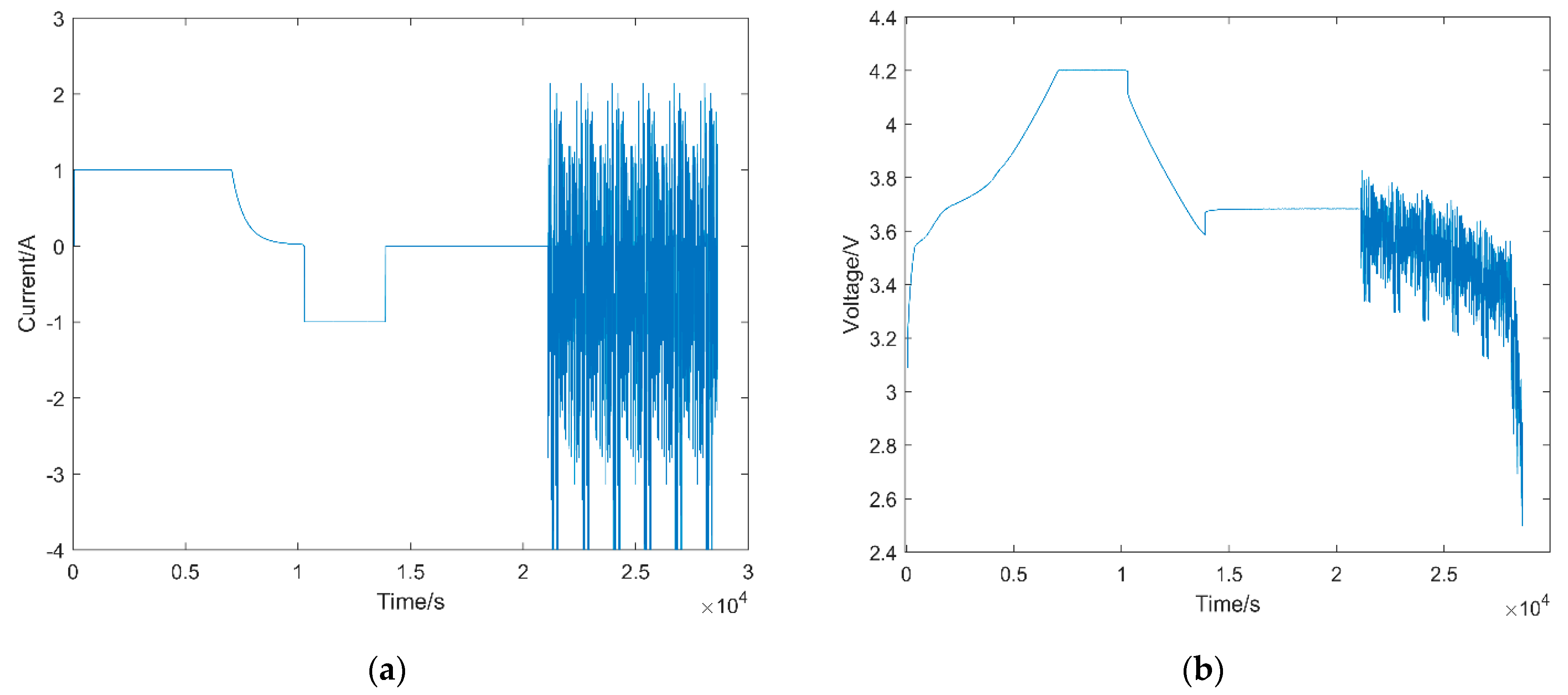
In this paper, we propose a method for lithium battery state-of-charge estimation based on Bayesian optimized bidirectional long- and short-term memory neural networks. The proposed method breaks the mold of traditional RNN studies that have been using only forward dependencies and further summarizes the temporal dependencies in the context of lithium battery sequence data by adding reverse dependencies. This study uses two publicly available lithium battery data sets, the CALCE data set, and the Oxford path-dependent battery degradation data set, and establishes mapping relationships between the observable voltage, current, and temperature variables of the battery and the battery SOC through the data provided by the data sets. The training results of different network models and a combination of previous experiences are used to determine the parameter intervals of the network, and then a Bayesian optimization algorithm is introduced to obtain the optimal parameters of the network. Through a large number of comparative experiments, including battery SOC estimation under different constant temperatures, a variable temperature environment, and different methods, the experimental results show that the proposed Bayes-BiLSTM model has a suitable fitting ability, and the SOC of batteries with different chemical compositions is estimated with higher accuracy and adaptability.

Future work will focus on verifying the applicability of the model for battery SOC estimation based on the collected data by adding a battery testing experimental platform; furthermore, the structure of the proposed model will be further improved to enhance its battery SOC estimation accuracy in low-temperature environments.

References

1. Chen, J.; Feng, X.; Jiang, L.; Zhu, Q. State of charge estimation of lithium-ion battery using denoising autoencoder and gated recurrent unit recurrent neural network. Energy 2021, 227, 120451. [Google Scholar] [CrossRef]
2. Duan, W.; Song, C.; Peng, S.; Xiao, F.; Shao, Y.; Song, S. An Improved Gated Recurrent Unit Network Model for State-of-Charge Estimation of Lithium-Ion Battery. Energies 2020, 13, 6366. [Google Scholar] [CrossRef]
3. Espedal Ingvild, B.; Asanthi, J.; Burheim Odne, S.; Lamb Jacob, J. Current Trends for State-of-Charge (SoC) Estimation in Lithium-Ion Battery Electric Vehicles. Energies 2021, 14, 3284. [Google Scholar] [CrossRef]
4. Chemali, E.; Kollmeyer, P.J.; Preindl, M.; Emadi, A. State-of-charge estimation of Li-ion batteries using deep neural networks: A machine learning approach. J. Power Sources 2018, 400, 242–255. [Google Scholar] [CrossRef]
5. Samarendra, P.S.; Praveen, P.S.; Sri, N.S.; Prabhakar, T. State of charge and health estimation of batteries for electric vehicles applications: Key issues and challenges. Glob. Energy Interconnect. 2021, 4, 145–157. [Google Scholar]
6. Rui, X.; Jiayi, C.; Quanqing, Y.; Hongwen, H.; Fengchun, S. Critical Review on the Battery State of Charge Estimation Methods for Electric Vehicles. IEEE Access 2018, 6, 1832–1843. [Google Scholar]
7. Li, Z.; Huang, J.; Liaw, B.Y.; Zhang, J. On state-of-charge determination for lithium-ion batteries. J. Power Sources 2017, 348, 281–301. [Google Scholar] [CrossRef] [Green Version]
8. Sun, D.; Yu, X.; Wang, C.; Zhang, C.; Huang, R.; Zhou, Q.; Amietszajew, T.; Bhagat, R. State of Charge Estimation for Lithium-Ion Battery based on an Intelligent Adaptive Extended Kalman Filter with improved noise estimator. Energy 2020, 214, 11199–11218. [Google Scholar] [CrossRef]
9. Deng, Z.; Yang, L.; Cai, Y.; Deng, H. Online Identification with Reliability Criterion and State of Charge Estimation Based on a Fuzzy Adaptive Extended Kalman Filter for Lithium-Ion Batteries. Energies 2016, 9, 472. [Google Scholar] [CrossRef] [Green Version]
10. Zhang, S.; Guo, X.; Zhang, X. An improved adaptive unscented kalman filtering for state of charge online estimation of lithium-ion battery. J. Energy Storage 2020, 32, 101980. [Google Scholar] [CrossRef]
11. Chen, J.; Lu, C.; Chen, C.; Cheng, H.; Xuan, D. An Improved Gated Recurrent Unit Neural Network for State-of-Charge Estimation of Lithium-Ion Battery. Appl. Sci. 2022, 12, 2305. [Google Scholar] [CrossRef]
12. Alvarez Anton, J.C.; Garcia Nieto, P.J.; Blanco Viejo, C.; Vilan Vilan, J.A. Support Vector Machines Used to Estimate the Battery State of Charge. IEEE Trans. Power Electron. 2013, 28, 5919–5926. [Google Scholar] [CrossRef]
13. Li, Y.; Sheng, H.; Cheng, Y.; Stroe, D.; Teodorescu, R. State-of-health estimation of lithium-ion batteries based on semi-supervised transfer component analysis. Appl. Energy 2020, 277, 115504. [Google Scholar] [CrossRef]
14. Liu, X.; Dai, Y. Energy storage battery SOC estimate based on improved BP neural network. J. Phys. Conf. Ser. 2022, 2187, 012042. [Google Scholar] [CrossRef]
15. Zhang, L.; Li, K.; Du, D.; Zhu, C.; Zheng, M. A sparse least squares support vector machine used for SOC estimation of Li-ion Batteries. IFAC Pap. 2019, 52, 256–261. [Google Scholar] [CrossRef]
16. Li, C.; Xiao, F.; Fan, Y. Approach to lithium battery SOC estimation based on recurrent neural network. J. Nav. Univ. Eng. 2019, 31, 107–112. [Google Scholar]
17. Li, S.; Ju, C.; Li, J.; Fang, R.; Tao, Z.; Li, B.; Zhang, T. State-of-Charge Estimation of Lithium-Ion Batteries in the Battery Degradation Process Based on Recurrent Neural Network. Energies 2021, 14, 306. [Google Scholar] [CrossRef]
18. Ephrem, C.; Kollmeyer Phillip, J.; Matthias, P.; Ryan, A.; Ali, E. Long Short-Term Memory Networks for Accurate State-of-Charge Estimation of Li-ion Batteries. IEEE Trans. Ind. Electron. 2018, 65, 6730–6739. [Google Scholar]
19. Li, C.; Xiao, F.; Fan, Y. An Approach to State of Charge Estimation of Lithium-Ion Batteries Based on Recurrent Neural Networks with Gated Recurrent Unit. Energies 2019, 12, 1592. [Google Scholar] [CrossRef] [Green Version]
20. Chong, B.; Shunkun, Y.; Jie, L.; Enrico, Z. Robust state-of-charge estimation of Li-ion batteries based on multichannel convolutional and bidirectional recurrent neural networks. Appl. Soft Comput. J. 2022, 116, 108401. [Google Scholar]
21. Bian, C.; He, H.; Yang, S. Stacked bidirectional long short-term memory networks for state-of-charge estimation of lithium-ion batteries. Energy 2020, 191, 116538. [Google Scholar] [CrossRef]
22. Feng, X.; Chen, J.; Zhang, Z.; Miao, S.; Zhu, Q. State-of-charge estimation of lithium-ion battery based on clockwork recurrent neural network. Energy 2021, 236, 121360. [Google Scholar] [CrossRef]
23. Alessandro, R.; Nicolò, G.; Antonio, C.; Matteo, B. Bayesian optimization and deep learning for steering wheel angle prediction. Sci. Rep. 2022, 12, 8739. [Google Scholar]
24. Xiong, X.; Guo, X.; Zeng, P.; Zou, R.; Wang, X. A Short-Term Wind Power Forecast Method via XGBoost Hyper-Parameters Optimization. Front. Energy Res. 2022, 10, 574. [Google Scholar] [CrossRef]
25. Cui, J.; Yang, B. Survey on Optimization Methodology and Applications. J. Softw. 2018, 29, 3068–3090. [Google Scholar]
26. Kollmeyer, P. Panasonic 18650pf li-ion battery data. Mendeley Data 2018. [Google Scholar] [CrossRef]
27. Raj, T.; Wang, A.A.; Monroe, C.W.; Howey, D.A. Investigation of Path-Dependent Degradation in Lithium-Ion Batteries. Batter. Supercaps 2020, 3, 1377–1385. [Google Scholar] [CrossRef]
28. Ren, X.; Liu, S.; Yu, X.; Dong, X. A method for state-of-charge estimation of lithium-ion batteries based on PSO-LSTM. Energy 2021, 234, 121236. [Google Scholar] [CrossRef]
Figure 1. LSTM network structure diagram.
Energies 15 04670 g001
Figure 2. Structure of the BiLSTM network.
Energies 15 04670 g002
Figure 3. Bayes-BiLSTM model structure.
Energies 15 04670 g003
Figure 4. Battery FUDS cycle test data at 45 °C: current (a) and voltage (b).
Energies 15 04670 g004
Figure 5. Experimental process.
Energies 15 04670 g005
Figure 6. Estimation results and errors of five BiLSTM models based on different numbers of hidden layer units.
Energies 15 04670 g006
Figure 7. SOC estimation of the Bayes-BiLSTM model at 45 °C: estimated results (a) and estimated errors (b).
Energies 15 04670 g007
Figure 8. SOC estimation of the Bayes-BiLSTM model at 25 °C: estimated results (a) and estimated errors (b).
Energies 15 04670 g008
Figure 9. SOC estimation of the Bayes-BiLSTM model at 0 °C: estimated results (a) and estimated errors (b).
Energies 15 04670 g009
Figure 10. Estimated results of BJDST in a variable temperature environment: estimated results (a) and estimated errors (b).
Energies 15 04670 g010
Figure 11. Comparison of the one-time battery SOC estimation results of different methods at 45 °C.
Energies 15 04670 g011
Figure 12. Estimation errors of different methods at 45 °C.
Energies 15 04670 g012
Figure 13. One-time half-cell SOC estimation results (a) and errors (b).
Energies 15 04670 g013