Theoretical Analysis of Active Flow Ripple Control in Positive Displacement Pumps

Abstract

Positive displacement machines present a well-known major drawback that is the oscillation in delivered flow rate. This paper presents two active solutions for reducing the flow ripple generated by a pump with an external device actuated by means of a piezo-stack actuator. The work is focused on a theoretical analysis, with the aim of collecting information about the performance of the solutions proposed and their main advantages and drawbacks. The active methods proposed involve a cylindrical actuator connected to the delivery line of the pump. The piston could be actuated directly by a piezo-stack actuator or by a differential pressure modulated by a proportional piezo actuated valve. The actuators were modelled and a control algorithm based on Least Mean Square algorithm was used to achieve the adaptability for both systems at different operating conditions. The developed mathematical model permits to define the great potential of these solutions that can drastically reduce the flow ripple. The first architecture presented resulted as the best solution, while the second one allowed reduction of the production cost.

1. Introduction

Positive displacement machines are commonly utilized in hydraulic circuits since they provide high power density together with robustness and reliability. However, one of the major drawbacks is the oscillation of the delivered flow rate, which in turn generates a pressure ripple and finally produces noise and vibrations that can cause stress to the components along the hydraulic circuit. This phenomenon can negatively affect durability and functionality of the hydraulic components [1]; furthermore, vibrations can affect the human being and environment [2].

Researchers dealing with the reduction in the flow and pressure ripple generated by positive displacement pumps have focused on different solutions, many of which contemplate the geometric optimization of components. In axial piston pumps, for example, a careful design of the port plate allows a smooth transition of the fluid pressure between suction and delivery phase and vice versa [3,4,5]. In gear pumps instead, side bushings are designed with particular grooves to improve the machine performance from this point of view [6,7,8,9,10,11].

Other methods involve devices external to the pump and could be classified as passive or active methods.

Passive methods contemplate fitting external devices, such as resonators, outside the pump. One major drawback of passive devices connected on a pump delivery line is that they usually are designed and set to operate in particular conditions, being effective only at certain pressures or against particular frequencies [12,13,14]. This means, for example, that if the pump shaft speed changes, these systems lose their effectiveness, with the pressure ripple frequency being determined directly by the pump rotational speed. In [13], a passive solution is proposed with the aim of reducing the pressure ripple both on the suction and on the delivery side; a particular flow ripple attenuator is presented and connected to suction and delivery lines.

To overcome passive method limitations, the solutions based on an active control can adapt themselves to the operating conditions in terms of fluid pressure and machine shaft speed. Researchers have also considered the combination of passive–active methods as reported in [12,14], where passive hoses are dedicated to the highest frequency reduction, while an active actuator acts on the main lower frequencies.

In particular, in [12,14] the presented solution is based on an actuator with a variable volume installed on the delivery side of the pump; the actuator acts by means of a piezoelectric actuator that is controlled with an adaptive filter with a feedforward algorithm.

Active methods are mostly based on generating a flow signal that superimposed to the pump delivery flow rate allows reduction of its oscillation: these solutions should generate a signal with a correct amplitude and phase to cancel the original one. The main drawback of active systems is that they are sophisticated devices that must be installed outside the pump, creating with it a relatively complex and bulky unit compared to the pump alone.

In [15], an active fluid borne noise attenuation has been applied to an aircraft hydraulic pump, the attenuator is an in-house rotary valve design, the pump and valve are shaft coupled so the effect of the speed is considered.

Focusing on axial piston pumps, the literature reports studies that aimed to reduce the amount of the structure-borne noise acting on the vibrations of the swash plate, that is controlled by a servo valve [16], while in [17,18] a similar solution is focused to compensate the uneven flowrate normally produced.

A similar solution is proposed in [19] where the swash plate is controlled to make adjustment to the instantaneous displacement. In [19], a second method is presented that uses a piezo stack to actuate a cylinder connected to the pump outlet.

In this paper, an active method to achieve flow ripple reduction in a positive displacement pump is presented. This method is based on an actuated piston placed on the delivery side of the pump that acts in counter phase with respect to the main flow ripple and it is able to significantly reduce the main harmonic of the flow oscillation.

The aim of this work is to move the first step of the research, so only a theoretical analysis is presented. The models of the two solutions were developed in Simcenter Amesim^TM environment. Two solutions for reducing the flow ripple are proposed, both based on the presence of a piston that, oscillating, generates a suitable flow. The difference between the two solutions is in the way the piston is actuated. This paper analytically presents the two solutions pointing out their advantages and disadvantages.

With the aim of making the two solutions able to adapt to changing pump working conditions, an adaptive control logic based on the LMS (Least Mean Square) algorithm was implemented to drive both active systems. The control logic was developed in Simulink^TM and cosimulation with the Amesim physical model was performed.

2. Description of the Active Methods

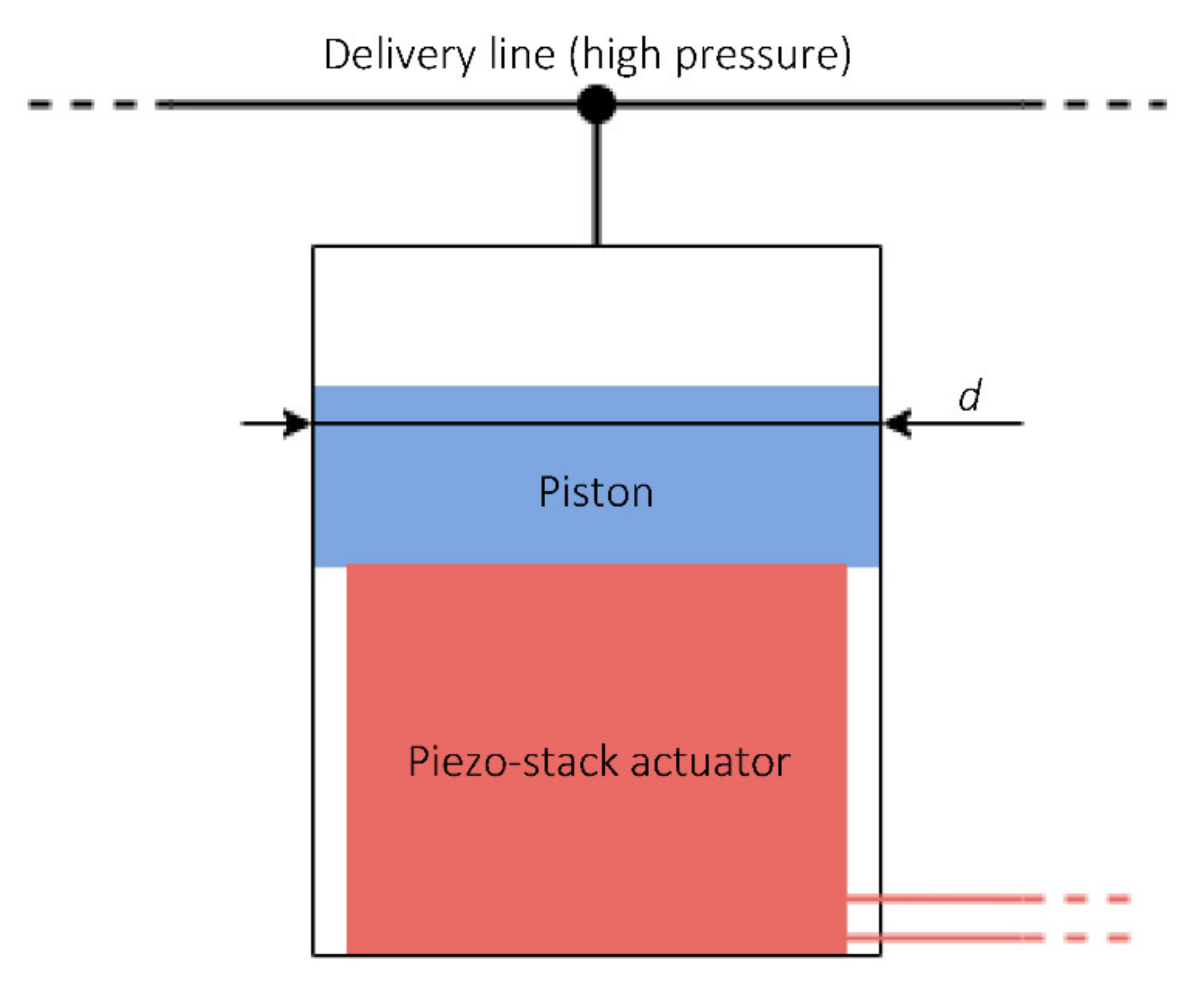
2.1. Piston Actuated by Piezo-Stack Actuator (1st Solution)

This active method of reducing the flow ripple, whose schematic is reported in Figure 1, involves a cylindrical actuator connected to the delivery line of the pump.

The piston is actuated by a piezo-stack actuator powered by an appropriate voltage amplifier with a feedforward logic signal based on the LMS algorithm. Thanks to this configuration, the entire system behaves like an adaptive filter that modulates its response according to the different operating conditions of the volumetric machine, adapting to variations in delivery pressure, flow rate, and rotation speed of the pump.

2.2. Hydraulically Actuated Piston (2nd Solution)

The second proposed active method is similar to the previous one, but a different solution was implemented to actuate the piston as shown in the schematic of Figure 2. In this solution, the piston is actuated by the fluid whose pressure is modulated by a three-way proportional valve, actuated by means of a piezo-stack actuator. The piston presents two cylindrical sections of different diameters.

The piston is housed in such a way to be in contact with a fluid at different pressure. The face of the piston with the larger diameter D is in contact with the volume A, directly connected to the delivery line of the hydraulic circuit. A spring is inserted to oppose the force that the fluid in A at delivery pressure generates on the piston. The chamber in which the spring is housed is connected to the tank and therefore no hydrostatic forces are generated on surfaces in contact with this chamber. The face with the smaller diameter d is in contact with volume B. Such a volume can alternatively be connected to the delivery or tank line by means of a three-way proportional valve. The valve is operated by means of a piezo-stack actuator powered by a suitable voltage amplifier. As for the first system, the control signal used to power the piezo actuator uses an LMS algorithm to implement a feedforward logic.

The active system operates as follows. When the piezo-stack actuator keeps the valve in position 1, as in the figure, the volume B is connected with delivery line and high-pressure fluid can flow into it pushing the piston upwards. With the upper side of the piston being of greater diameter than the lower side, the total contribution of this phase is a release of fluid towards the delivery line. Then, when the piezo stack actuator brings the valve in position 2, chamber B is connected to low pressure tank line where the fluid can flow while the piston comes back down, pushed by the delivery pressure that acts on the greater side of the piston.

The piezo-stack actuator used in this method to operate the valve can be smaller than the one used in the first method, because it does not have to act directly against the delivery pressure and so it has to withstand a definitely lower force.

In the operation of this active system, the drainage of a certain amount of fluid is expected. In fact, as it has been explained, at each switching cycle of the piezo-actuated valve a small volume of pressurized fluid is diverted from the pump delivery into volume B to allow the piston to be actuated and then released towards the tank to depressurize the volume. The drainage obtained is, however, modest as found thanks to the developed model.

3. Sizing and Definition of Active System Operating Parameters

3.1. Piston Actuated by Piezo-Actuator (1st Solution)

The piston and the piezo-actuator were sized starting from the analysis of the flow ripple generated by the pump. By integrating the flow rate oscillating component in the time domain, it is possible to obtain the fluid volume that the piston should move at each pulsation of the piezo-actuator to completely cancel the flow ripple. As shown in Figure 3, the aforementioned volume V is obtained as the peak-to-peak value of the integral of flow ripple.

The volume V was identified starting from the flow ripple generated by the pump at its most difficult working conditions. This is to ensure that the active system is effective in the whole working range of the pump, even in the most severe conditions.

Naming d the piston diameter and s the maximum displacement of the piezo-stack actuator, which corresponds to the stroke of the piston, it is possible to relate these two parameters thanks to the fluid volume V that must be handled by the piston:

$$V=s·\pi \frac{d^2}{4}$$

(1)

from which d can be written as a function of s:

$$d=\sqrt{\frac{4V}{\pi s}}$$

(2)

The diameter d depends the load F on the piston and the actuator at a fixed pressure p. When the pressure is at its maximum, p_max, the load is also at its maximum F_max, and writing d as a function of s as in the (2) it is possible to obtain

$$F_{max}=p_{max}·\frac{V}{s}$$

(3)

The piezo-stack actuator used to actuate the piston should then be able to withstand such a load.

3.2. Hydraulically Actuated Piston

For the active method with a hydraulically actuated piston, the sizing and definition of the operating parameters are more difficult due to the complex interaction between the different elements that make up the system. For this reason, the sizing was performed through successive optimization steps, carried out using the optimization tools available in the Amesim software. The parameters subject to optimization are the upper diameter of the piston D, the lower diameter of the piston d, and the stiffness of the spring coupled to the piston. The goal of the optimization is to maximize the reduction of the first harmonic of the flow ripple, containing at the same time the drainage of the fluid that occurs, as explained above, during the operation of this device.

The Amesism tool used to perform this optimization relies on the NLPQL (Non-Linear Programming by Quadratic Lagrangian) optimization algorithm.

4. Mathematical Model

4.1. Fluid Model

A simple fluid model was used to represent the hydraulic working fluid, gas/vapor release is not taken into account since the pressure at the delivery side of the pump always stays well above the cavitation threshold. The temperature was considered constant and equal to T = 50 °C. Density was calculated as a function of pressure variation considering the liquid bulk modulus β:

$$\rho ={\rho }_0·\left[1+1/\beta ·\left(p-p_0\right)\right]$$

(4)

4.2. Pump Model

With the aim of generating a flow ripple to test the two active solutions, a pump model was used. The pump mathematical model adopted in this study is based on the axial piston pump Amesim submodel. This already available model permitted the authors to focus the research only on the active solutions for reducing the flow ripple. A brief description of the model is presented. The pump is treated as a series of interconnected open volumes according to the Filling and Emptying concept.

The pressure in every chamber is obtained by integrating the pressure time derivative considering the volumes as capacitive elements:

$$\frac{dp}{dt}=\frac{\beta }{\rho }\frac{1}{V\left(t\right)}\left(\sum \dot{m}-\rho \frac{dV\left(t\right)}{dt}\right)$$

(5)

where ρ is the fluid density, β is the bulk modulus, V(t) the instantaneous volume of the chamber, $\dot{m}$ is the flow rates from the inlet port and to the outlet port, respectively. Flow rates going through inlet and outlet ports for every volume chamber are computed with the orifice law:

$$\dot{m}=c_{q}A\left(t\right)\rho \sqrt{\frac{2\left|\Delta p\right|}{\rho }}$$

(6)

where c_q is the discharge coefficient and A(t) is the flow area.

The geometrical features of the simulated pump were used to define all geometrical parameters needed by the Amesim axial piston pump mathematical submodel.

The target of the pump model is only to generate a typical flow ripple of a positive displacement pump, in this particular case axial piston pumps were considered. Figure 4 and Figure 5 report the output flow ripple of the model and its Fast Fourier Transform (FFT), respectively.

4.3. Piezo-Stack Actuator Model

The piezoelectric actuator model was simulated with the Amesim linear piezoelectric stack actuator submodel.

In this model, the force F and the voltage U applied to the piezo-stack actuator are related to the displacement dZ and the electric charge dQ by the following relation:

$$\left(\begin{array}{c}F\\ U\end{array}\right)=\left(\begin{array}{cc}{K}_{11}& K_{12}\\ K_{21}& K_{22}\end{array}\right)·\left(\begin{array}{c}dZ\\ dQ\end{array}\right)$$

(7)

Thanks to typical the piezo-stack actuator specifics (electrical capacitance, closed circuit stiffness, blocking load), it is possible to obtain the parameters K11, K12, K21, and K22 that determine the functioning.

The described model is simplified in comparison to the complexity of a real piezo-stack actuator. In fact, the model does not take into account either hysteresis effects or the dependence of the piezo-stack electrical capacitance on the temperature and operating frequency. If hysteresis effects can be neglected for this study, the variation in electrical capacitance must be considered. In fact, an increase in electrical capacitance is the cause of a decrease in the piezo-stack actuator ability to respond to high frequency control signals, as illustrated in Section 4.4. For this reason, in the model, an electrical capacitance overestimated by a safety factor is used.

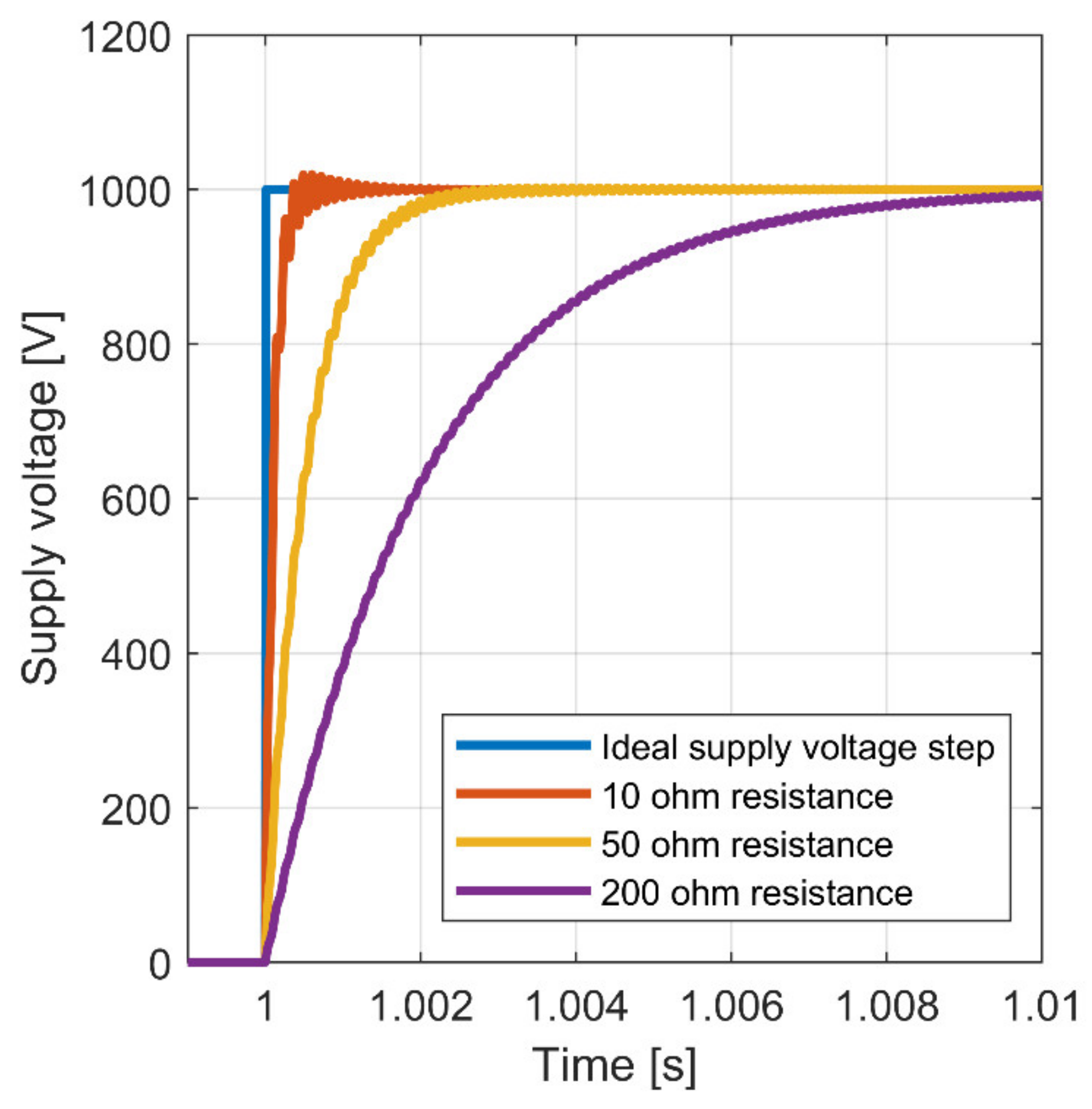
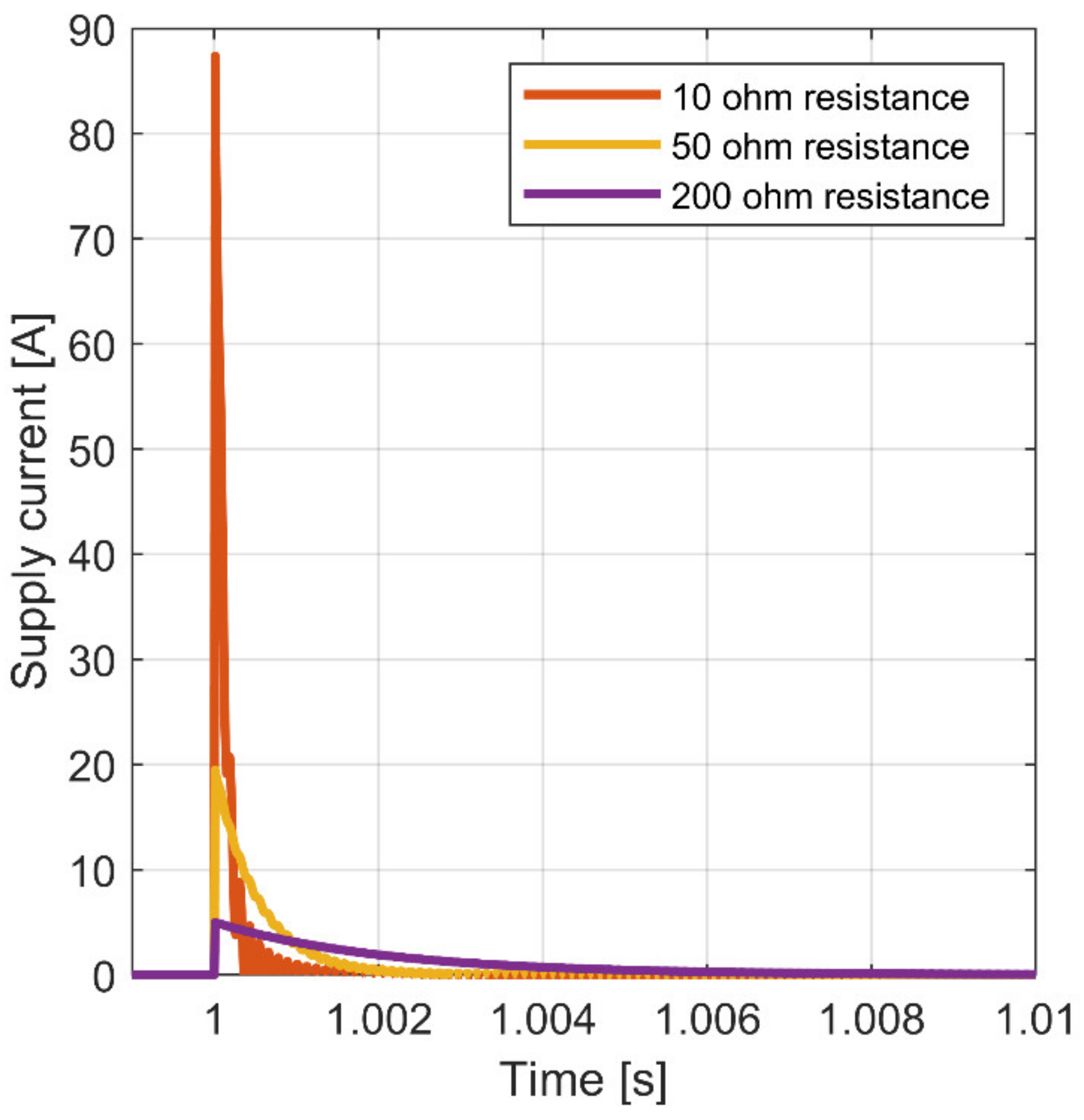
4.4. Piezo-Stack Actuator Power Supply

The high performance piezo-stack actuators considered for this study are characterized by an operating voltage assumed to be in the range of 0–1000 V. To achieve this voltage, a high-power amplifier must be used.

Assuming that the power amplifier has a maximum output current, therefore, current must be limited to stay below this threshold, the current limitation is the cause of delay and reduction in the power amplifier response to the control signal. In fact, having the piezo-stack actuator at a considerable electric capacitance, a certain amount of time is required for the voltage to build up at its ends in case of a limited charge current. The electrical circuit in which the piezo-stack actuator is plugged in behaves, therefore, like an RC circuit, as shown in Figure 6.

To ensure that the current stays below the maximum threshold imposed by the power amplifier, an electrical resistance is needed, connected in series with the piezo-stack actuator. The resistance must be sized to be as small as possible because an excessive reduction in the power amplifier output current brings a greater response delay and a high frequency performance loss.

In Figure 7 and Figure 8, it is possible to see the influence of the electrical resistance on the power amplifier current and on the voltage imposed to the piezo-stack actuator when a 0–1000 V step is used as the control signal on the system.

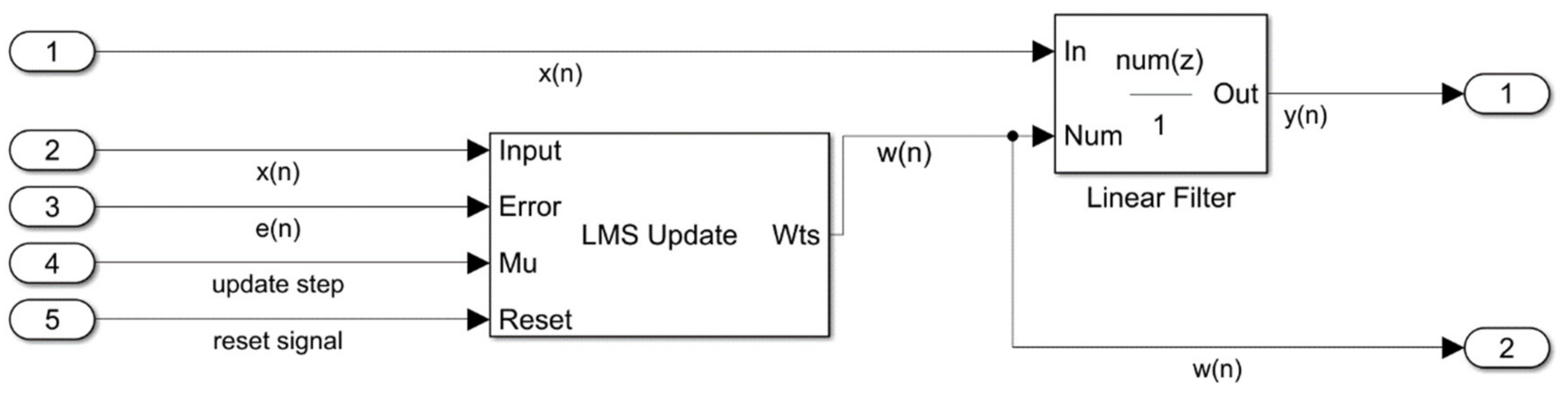
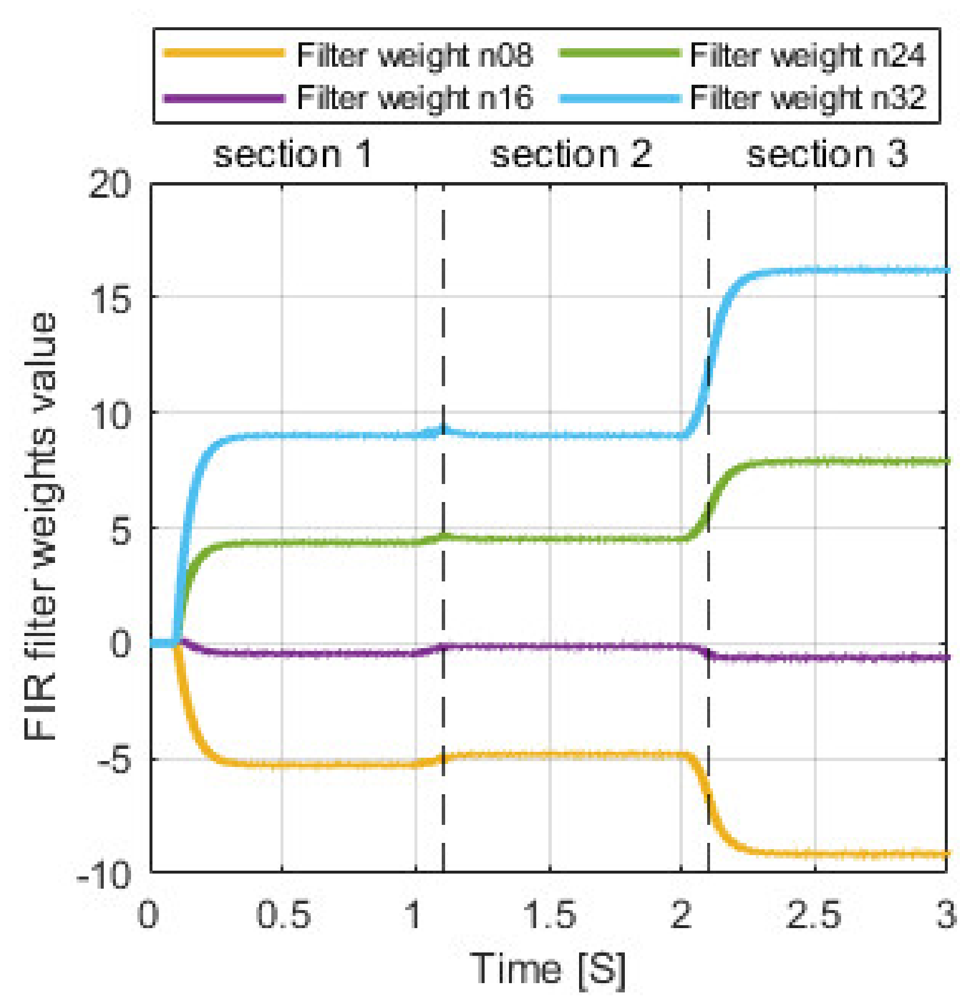
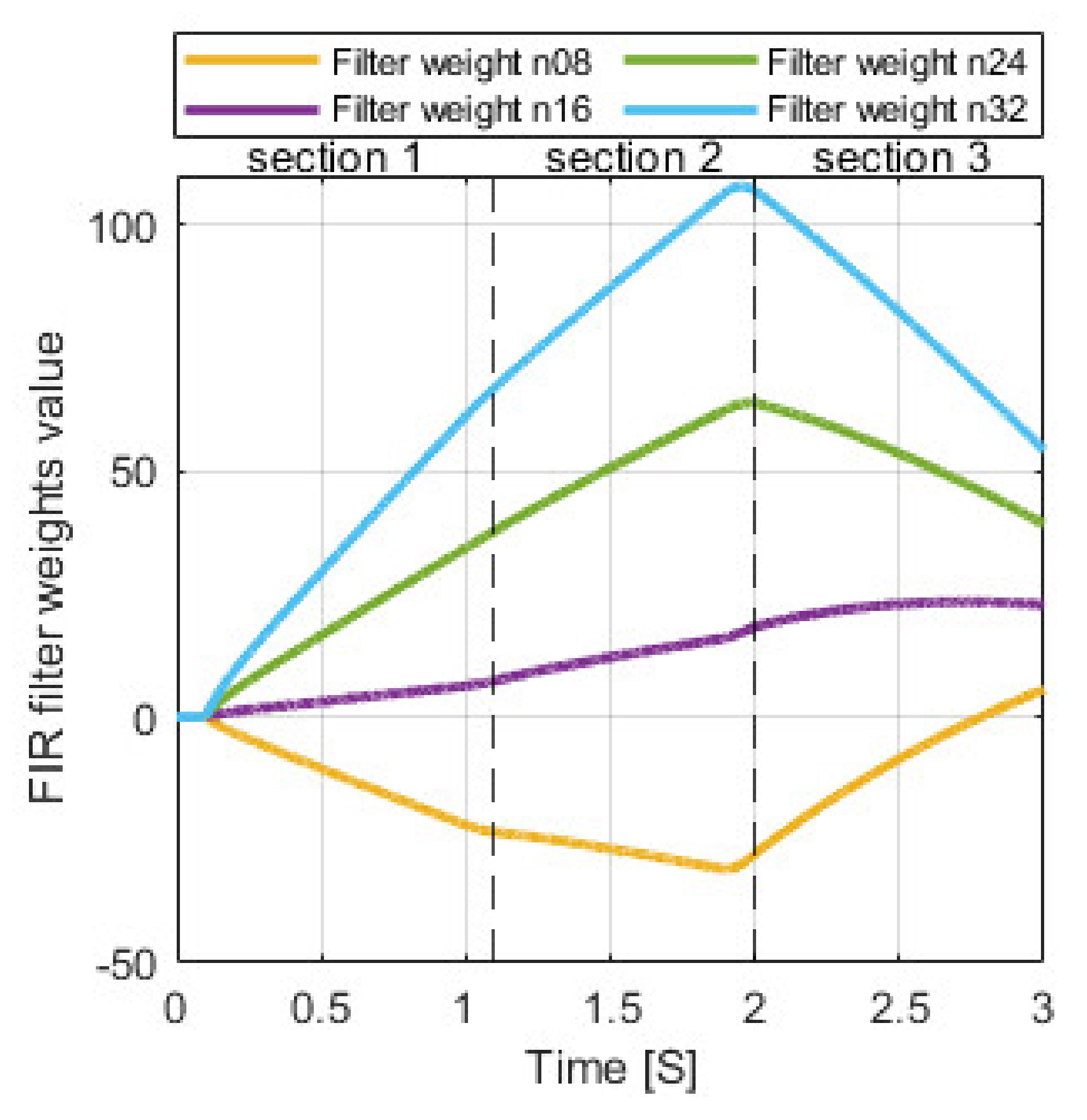
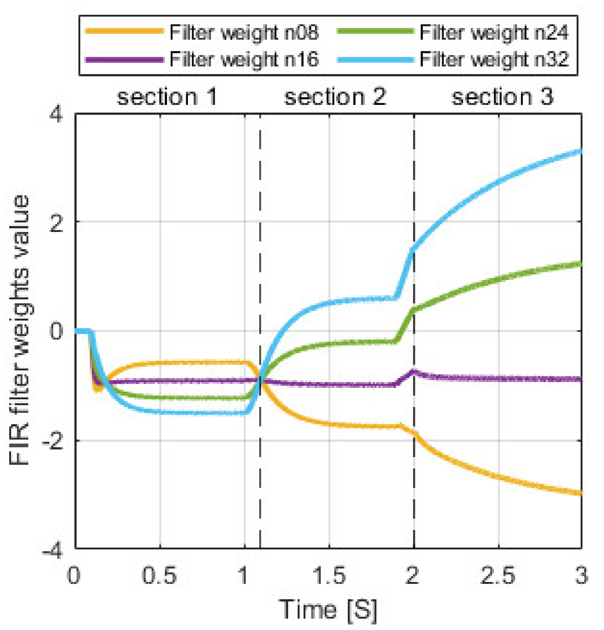
5. Control Algorithm Model

The active systems are controlled to behave like adaptive filters, which are FIR (Finite Impulse Response)-type filters whose parameters are constantly updated through a specific algorithm. In this case, the algorithm used is the LMS (least Mean Square) algorithm. The scheme of a generic adaptive filter is reported in Figure 9.

The adaptive algorithm is fed with an input signal x(n), which is a sinusoid having the same frequency of the error signal e(n) pulsation that must be reduced. The adaptive algorithm computes the parameters used by the linear filter to minimize the error signal.

The aforementioned linear filter is fed with x(n) input signal and gives a cancellation signal y(n) as output. y(n) is subtracted from d(n) which is the actual pump flow rate containing the desired average value and the unwanted oscillating component.

The error signal e(n) used to feed the adaptive filter is the pressure ripple measured at pump delivery and cleaned of the average value by means of a high-pass filter.

The LMS algorithm was implemented in the Simulink environment using two blocks: the LMS update block, which outputs the weights used as input in the Linear Filter block, as shown in Figure 10. The FIR linear filter length, N, was set to 32, which means that it is composed of 32 filter weights w(n) that are constantly updated thanks to the LMS block.

In LMS algorithm, the updating of the N filter weights w(n) happens as follows:

$$w{\left(n+1\right)}_k=w{\left(n\right)}_K+\mu e\left(n\right)x\left(n-K\right),\hspace{1em}\hspace{1em}K=0, 1, \dots , N-1$$

(8)

where K is the index of the filter weight and μ is the update step size that must be large enough to provide fast convergence of the filter weights and at the same time small enough to ensure algorithm stability.

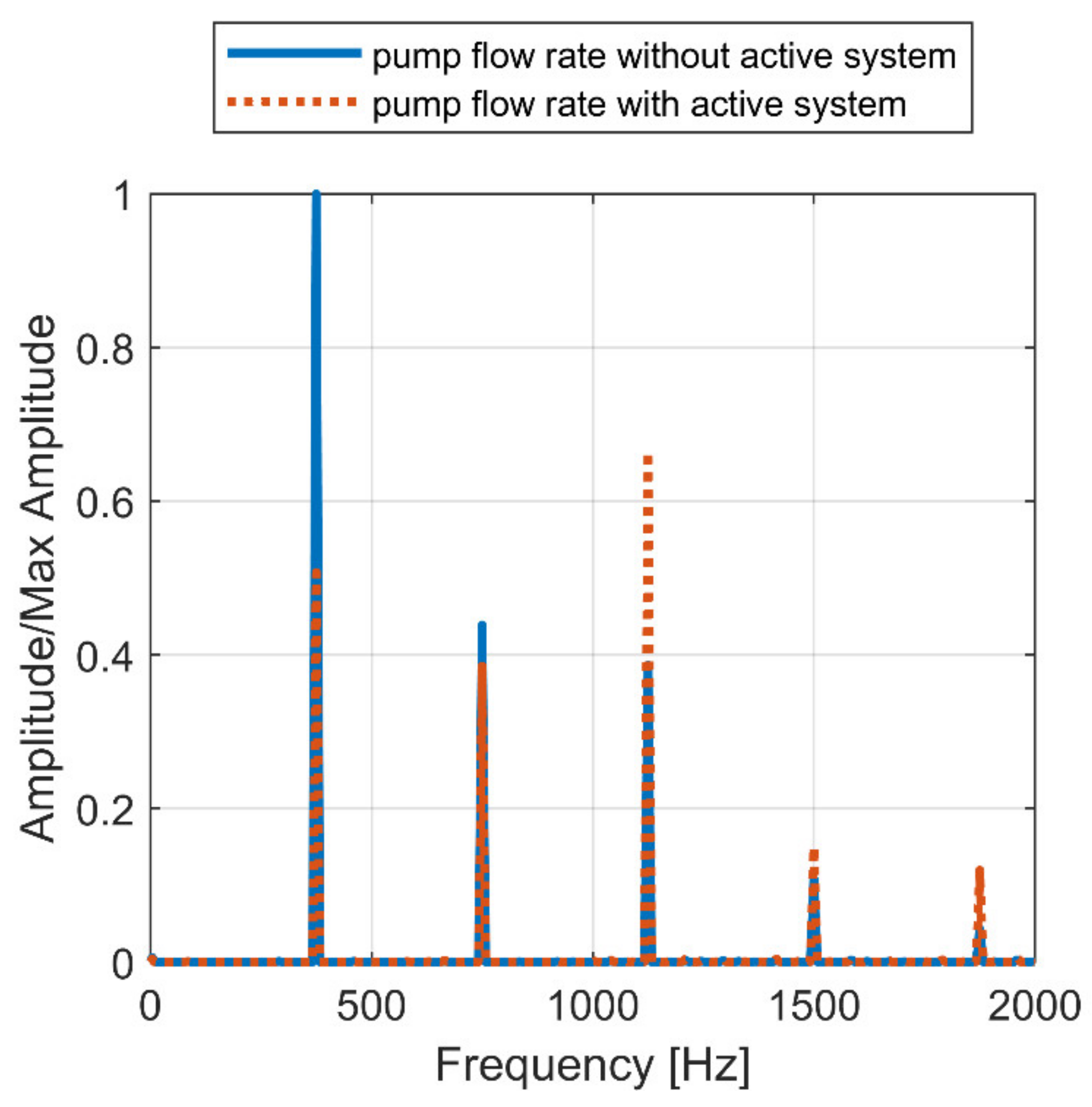
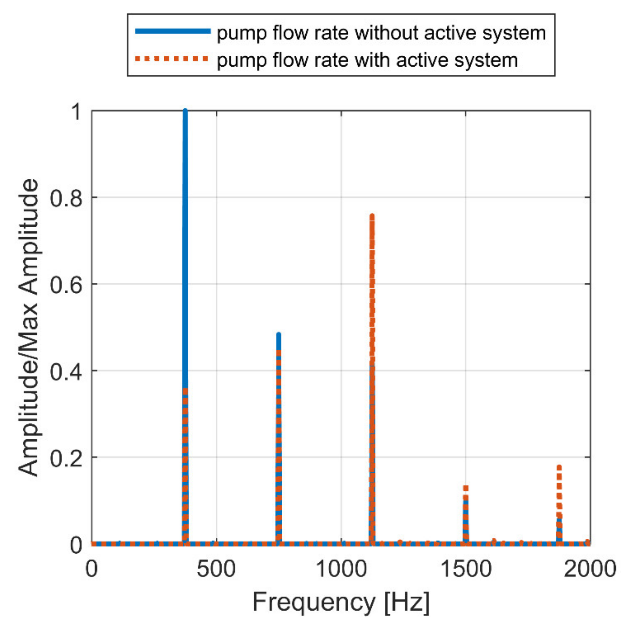
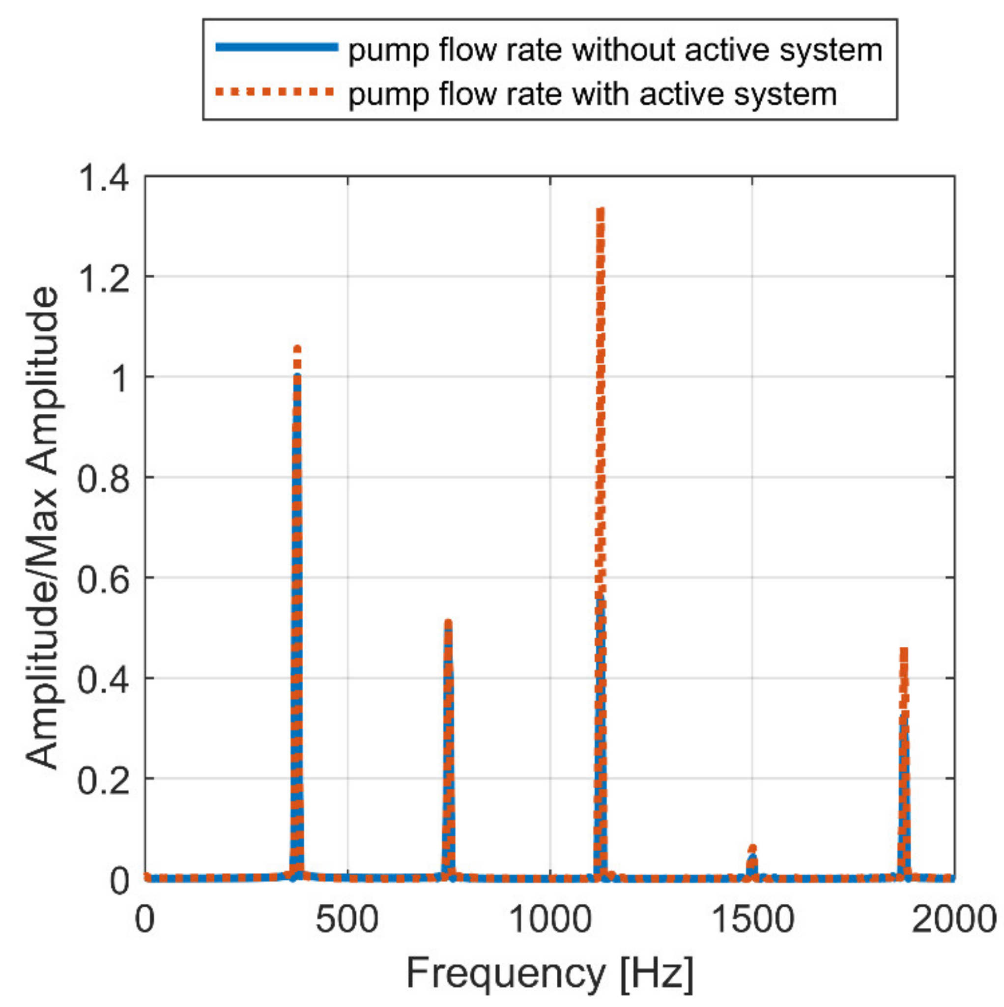
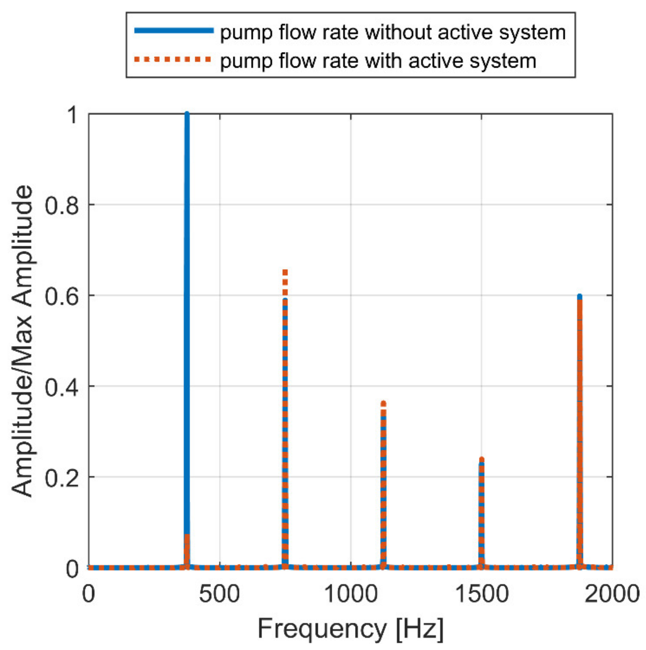
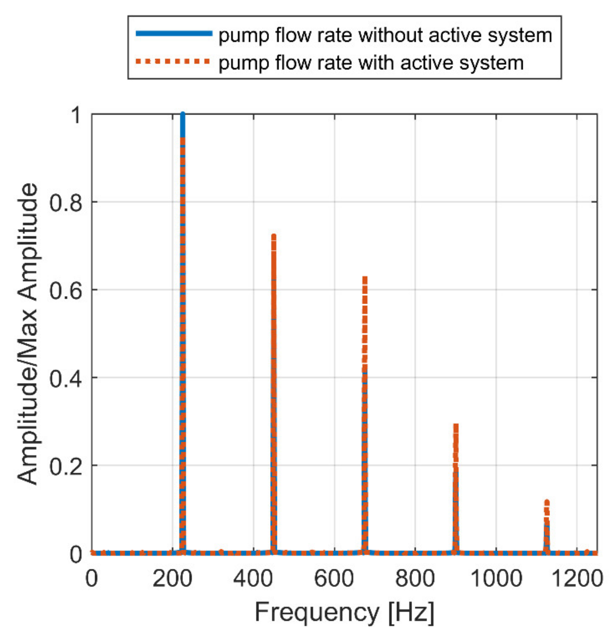
6. Simulations Results

Simulations of the operation of the two studied active flow ripple cancellation systems were carried out with the aim of verifying their effectiveness for different working conditions of the positive displacement pump. In particular, the target was to evaluate the capacity to reduce the flow ripple and the ability to adapt to different conditions of the delivery pressure, delivered flow rate, and rotation speed of the volumetric pump.

Simulations consist of imposing different working cycles to the pump during which operating conditions change. Precisely, two different cycles were tested, each composed of three steady sections characterized by different pressure, pump speed, and swash plate angle.

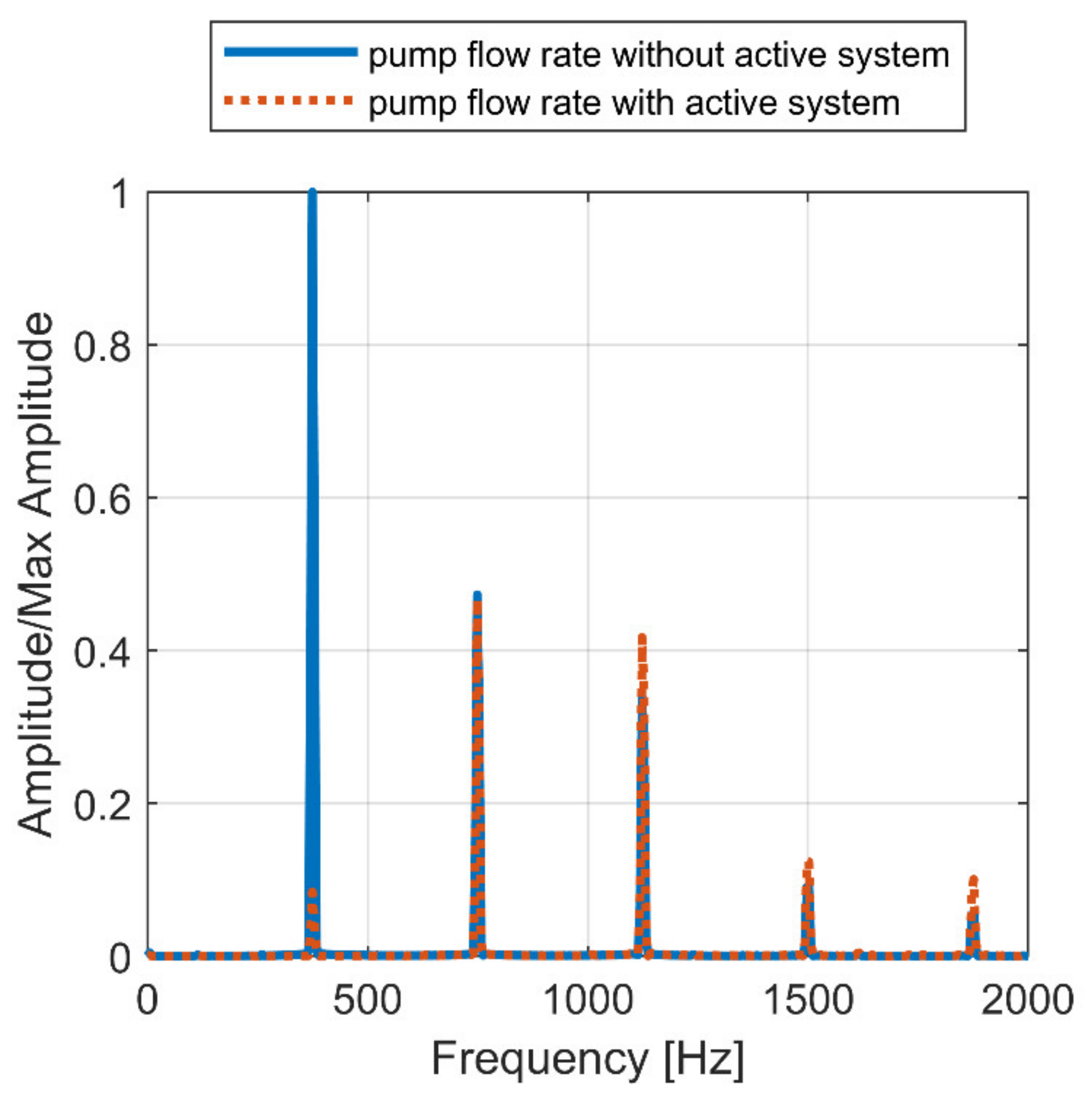
6.1. Piston Actuated by Piezo-Actuator (1st Solution)

In the first run, the pump working cycle was set as shown in

Table 1. Pump working conditions in first simulation cycle.

Cycle Section	1	2	3
Average delivery pressure [bar]	250	135	30
Pump rotation speed [rpm]	2500	2500	2500
Swash plate angle/max. angle [%]	100	100	50
Average flow rate [L/min]	200	200	100

.

Between every steady-state section, a short transition section was also inserted to allow the working conditions to change smoothly.

In Figure 11, Figure 12 and Figure 13, the FFT of pump delivery flow rate in the three steady-state conditions is reported. It is possible to see the effect of flow ripple reduction produced by the active system comparing the main harmonic amplitude with and without active system intervention.

In each one of the three cycle sections, the first order harmonic of the flow ripple is clearly reduced. The reduction amounts to 89% for cycle section 1, to 92% for section 2, and to 95% for section 3.

It is possible to note that higher order harmonics may show a small increase or decrease even if the active system is meant to act only on the first main one. This is attributable to the introduction of the active system that brings with it small changes in the delivery line characteristics, like fluid volume for example, modifying the frequency response of the hydraulic system. This phenomenon can be seen in all the other simulated conditions, for which the aforementioned explanation remains valid.

The active method also shows good performances in autonomously updating the control system parameters to adapt to pump working condition changes. In Figure 14, 4 of the 32 weights of the FIR filter updated with the LMS algorithm during simulation are shown. Only 4 weights are reported for simplicity. As it can be seen from the graph, each weight converges rapidly to a new value after the working condition changes. Convergence time is in the order of tenths of a second.

Since in the first run cycle only constant speed and decreasing pressure situations were tested, the second run cycle contemplates a decrease in pump speed between sections 1 and 2 and an increase in pressure between sections 2 and 3, as it can be seen in

Table 2. Pump working conditions in second simulation cycle.

Cycle Section	1	2	3
Average delivery pressure [bar]	250	90	220
Pump rotation speed [rpm]	2500	1500	1500
Swash plate angle/max. angle [%]	100	100	100
Average flow rate [L/min]	200	120	120

.

In Figure 15, Figure 16 and Figure 17, results referring to the simulated cycle indicated in Table 2 are reported. Results regarding section 1 are not reported because the section 1 of the second cycle has the same parameters of the section 1 of the first cycle. From the results, it is possible to state that also in conditions of variable pump speed and increasing delivery pressure the control algorithm can allow the active system to adapt to varying pump working conditions. Flow ripple first harmonic reduction for sections 1–3 amounts, respectively, to 89%, 82%, and 74%.

During functioning of the active system, the supply current of the piezo stack actuator reaches very high values of over 8 A. The characteristic power supply maximum current of a piezo-actuator is usually below this value; for this reason, it was decided to limit the supply current by appropriately increasing the electrical resistance placed in series with the piezo-actuator, in order to maintain peak current below the 6 A threshold.

A simulation was run with pump working cycle identical to the first run (Table 1) to compare effectiveness with and without electric current limitation. Results are reported in Figure 18, Figure 19, Figure 20 and Figure 21.

With the supply current limited to 6 A, the effectiveness of the active system, as currently dimensioned, is significantly reduced with respect to the case with higher current. In addition, the adaptive algorithm is no more capable of successfully updating the FIR filter weights that now tend to diverge, explaining why flow ripple reduction cannot be achieved.

A possible solution to this problem is represented by using a greater number of piston–actuator pairs, to use smaller piezo-stack actuators which are provided with a higher bandwidth requiring a smaller supply current. Another possible solution is to design an ad hoc power supply, capable of providing peak currents suitable for making the application effective. However, both solutions would be very expensive, making the system grow in complexity and costs.

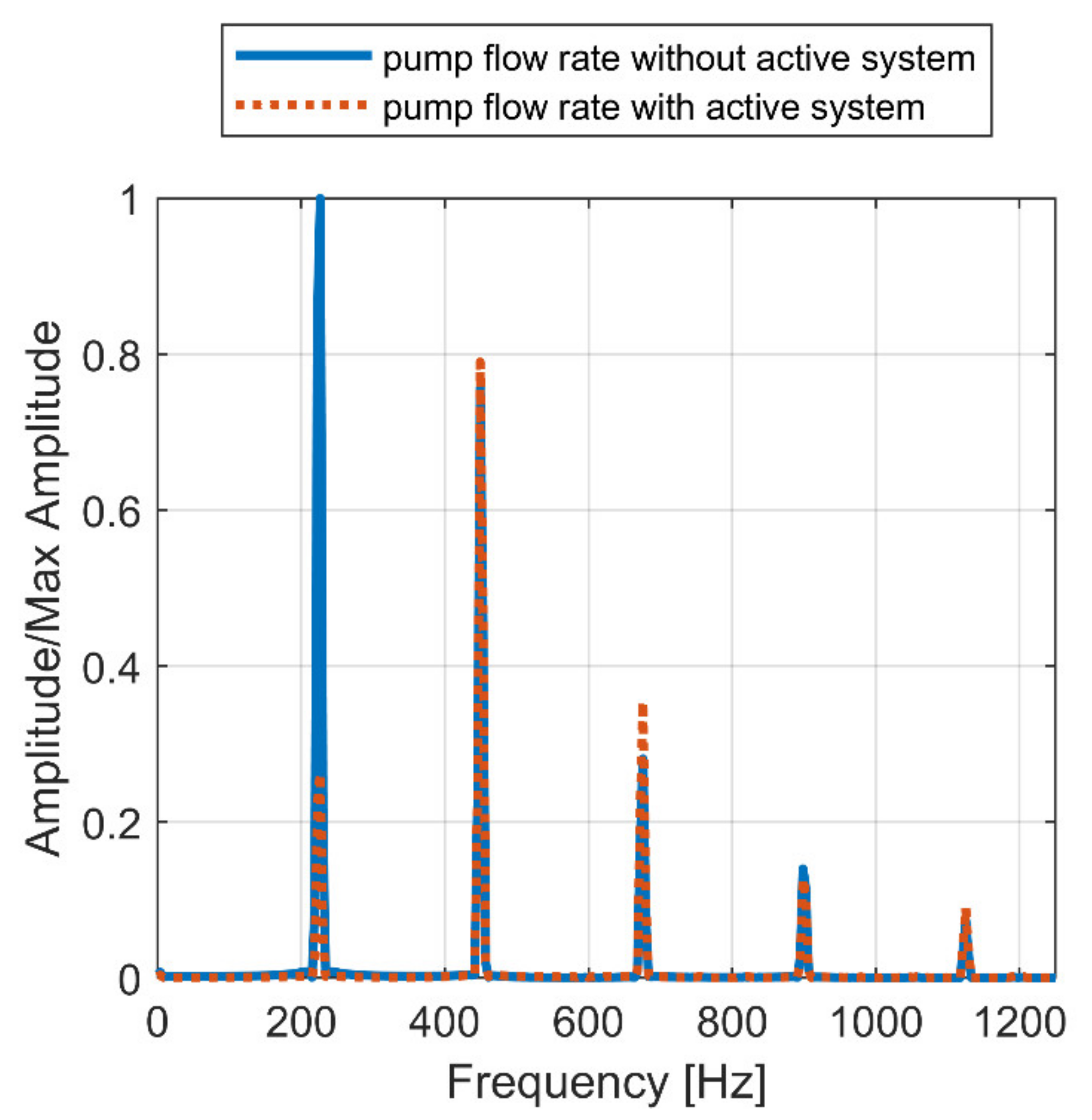
6.2. Piston Actuated Hydraulically via Piezo-Valve (2nd Solution)

The same working cycles used for the 1st solution were applied to the 2nd solution which relies on a piezo-valve to hydraulically actuate the piston.

In Figure 22, Figure 23, Figure 24 and Figure 25, results referring to the first cycle stage (Table 1) are reported. The reduction in the first harmonic of flow ripple is clearly effective, reaching values of 97% in section 1 of the cycle, 96% in section 2, and 93% in section 3. However, convergence in FIR filter weights appears to be slower if compared to the 1st piezo-actuated active system case. In particular, in section 3 of the cycle, filter weight stable values were not reached in 1 s time, and therefore it is possible to see that they are still updating when the simulation stops, with their trend still sloping.

In Figure 26, Figure 27 and Figure 28, results referring to the second cycle pattern (Table 2) are reported. Results regarding section 1 are not reported because the section 1 of the second cycle has the same parameters of the section 1 of the first cycle. In this case, it is possible to see by the trend of the FIR filter weights that the control algorithm is not able to keep up with changing working conditions of the pump. In particular, after being able to converge in the first section of the cycle, filter weights then rapidly diverge starting from the section number 2, compromising the effectiveness of the active system.

One possible explanation for the unwanted behavior of the 2nd active system control algorithm is the fact that the control signal generated by the FIR block and the piston actual movement is not correlated as strongly as in the 1st active system presented. In the 2nd system, the control signal operates a piezo-valve which has an influence on the piston oscillation, but the correlation is much smaller than in a control signal directly operating the piston through a piezo-stack actuator as in the 1st active system.

The LMS algorithm needs a strong correlation between the generated control signal and the effective cancellation signal to function properly. In this second active system, the oscillation of the piston, which actually produces the flow ripple cancellation signal, depends strongly on the average delivery pressure and on the first harmonic of the flow ripple. As a consequence, the algorithm is not able to adapt itself promptly when the pump working condition changes.

The quantity of fluid drained in the operation of this active system is acceptably small, never exceeding 1.5% of the pump delivery flow rate in any of the simulated operating conditions.

7. Conclusions

In this paper, two active methods to achieve pump flow ripple reduction were proposed. Both methods rely on pistons producing flow ripple cancellation signals, one involving a direct piezo-actuated piston and the second involving a piston actuated hydraulically via a piezo-valve. Mathematical models of the two methods were presented, including a control algorithm used to achieve adaptability for both systems.

Both methods can be applied to any kind of positive displacement pump, even if for this work an axial piston pump was used for simulation purposes.

Results of numerical simulations were discussed, showing the potentialities and problems of the two proposed methods.

In particular, it was demonstrated how the first active solution can heavily reduce the flow ripple and effectively adapt to changing working conditions, as long as a sufficient supply current is available. Thanks to this active system, in fact, the reduction of 80–90% of the flow ripple main harmonic was achieved.

The second active method permits to avoid some of the first method disadvantages. In fact, a smaller piezo-stack actuator is needed to operate the valve reducing the cost and dimensions and preventing high supply current related problems. However, with the method being more complex, the control algorithm has to be improved to allow the active system to reliably adapt to pump working condition changes. However, this active system was proved to be promising, achieving reduction of the flow ripple main harmonic of over 90% when correctly functioning, implying only a small fluid drainage of 1.5% of pump delivery flow.

Regarding future developments on the research presented in this paper, the next step will be the design and optimization of more stable and reliable control algorithms, working on the basis represented by the one used for this research. Then, prototypes of the two solutions presented will be designed and an experimental campaign will be performed to validate simulation results.

References

1. Karpenko, M.; Prentkovskis, O.; Šukevičius, Š. Research on high-pressure hose with repairing fitting and influence on energy parameter of the hydraulic drive. In Eksploatacja i Niezawodnosc—Maintenance and Reliability; Polish Maintenance Society: Lublin, Poland, 2022; Volume 24, pp. 25–32. ISSN 1507-2711. [Google Scholar]
2. Stosiak, M. The impact of hydraulic systems on the human being and the environment. J. Theor. Appl. Mech. 2015, 53, 409–420. [Google Scholar] [CrossRef] [Green Version]
3. Ye, S.; Zhang, J.; Xu, B. Noise Reduction of an Axial Piston Pump by Valve Plate Optimization. Chin. J. Mech. Eng. 2018, 31, 57. [Google Scholar] [CrossRef] [Green Version]
4. Johansson, A.; Olvander, J.; Palmberg, J.-O. Experimental verification of cross-angle for noise reduction in hydraulic piston pumps. Proc. Inst. Mech. Eng. Part I J. Syst. Control Eng. 2007, 221, 321. [Google Scholar] [CrossRef]
5. Harrison, A.M.; Edge, K. Reduction of axial piston pump pressure ripple. Proc. Inst. Mech. Eng. 2000, 214, 53–64. [Google Scholar]
6. Borghi, M.; Zardin, B. Axial Balance of External Gear Pumps and Motors: Modelling and Discussing the Influence of Elastohydrodynamic Lubrication in the Axial Gap. In Proceedings of the ASME International Mechanical Engineering Congress and Exposition, Houston, TX, USA, 13–19 November 2015. [Google Scholar] [CrossRef] [Green Version]
7. Zhao, X.; Vacca, A. Theoretical investigation into the ripple source of external gear pumps. Energies 2019, 12, 535. [Google Scholar] [CrossRef] [Green Version]
8. Zhao, X.; Vacca, A. Numerical analysis of theoretical flow in external gear machines. Mech. Mach. Theory 2017, 108, 41–56. [Google Scholar] [CrossRef]
9. Zhou, J.; Vacca, A.; Casoli, P. A Novel Approach for Predicting the Operation of External Gear Pumps Under Cavitating Conditions. Simul. Model. Pract. Theory 2014, 45, 35–49. [Google Scholar] [CrossRef]
10. Rundo, M.; Altare, G.; Casoli, P. Simulation of the filling capability in vane pumps. Energies 2019, 12, 283. [Google Scholar] [CrossRef] [Green Version]
11. Corvaglia, A.; Ferrari, A.; Rundo, M.; Vento, O. Three-dimensional model of an external gear pump with an experimental evaluation of the flow ripple. Proc. Inst. Mech. Eng. Part C J. Mech. Eng. Sci. 2021, 235, 1097–1105. [Google Scholar] [CrossRef]
12. Pan, M.; Ding, B.; Yuan, C.; Zou, J.; Yang, H. Novel Integrated Control of Fluid-Borne Noise in Hydraulic Systems. In Proceedings of the BATH/ASME 2018 Symposium on Fluid Power and Motion Control FPMC 2018, Bath, UK, 12–14 September 2018. [Google Scholar]
13. Shang, Y.; Tang, H.; Sun, H.; Guan, C.; Wu, S.; Xu, Y.; Jiao, Z. A novel hydraulic pulsation reduction component based on discharge and suction self-oscillation: Principle, design and experiment. Proc. Inst. Mech. Eng. Part I J. Syst. Control Eng. 2020, 234, 433–445. [Google Scholar] [CrossRef]
14. Pan, M.; Johnston, N.; Plummer, A. Hybrid Fluid-borne Noise Control in Fluid-filled Pipelines. J. Phys. Conf. Ser. 2016, 744, 012016. [Google Scholar] [CrossRef] [Green Version]
15. Waitschat, A.; Thielecke, F.; Behr, R.M.; Heise, U. Active Fluid Borne Noise Reduction for Aviation Hydraulic Pumps. In Proceedings of the 10th International Fluid Power Conference, Dresden, Germany, 8–10 March 2016. [Google Scholar]
16. Kim, T.; Ivantysynova, M. Active Vibration/Noise Control of Axial Piston Machine Using Swash Plate Control. In Proceedings of the ASME/BATH 2017 Symposium on Fluid Power and Motion Control, Sarasota, FL, USA, 16–19 October 2017; Paper No. FPMC2017-4304. p. V001T01A053. [Google Scholar] [CrossRef]
17. Casoli, P.; Pastori, M.; Scolari, F.; Rundo, M. Active pressure ripple control in axial piston pumps through high-frequency swash plate oscillations—A theoretical analysis. Energies 2019, 12, 1377. [Google Scholar] [CrossRef] [Green Version]
18. Casoli, P.; Pastori, M.; Scolari, F. Swash plate design for pressure ripple reduction—A theoretical analysis. In Proceedings of the AIP Conference, Modena, Italy, 11 September 2019. [Google Scholar] [CrossRef]
19. Hagstrom, N.; Harens, M.; Chatterjee, A.; Creswick, M. Piezoelectric actuation to reduce pump flow ripple. In Proceedings of the ASME/BATH 2019 Symposium on Fluid Power and Motion Control 2019 FPMC, Sarasota, FL, USA, 7–9 October 2019. [Google Scholar]
Figure 1. Schematic of piezo-stack actuated piston active method.
Energies 15 04703 g001
Figure 2. Schematic of hydraulically actuated piston active method.
Energies 15 04703 g002
Figure 3. Simulated pump delivery flow ripple and its integral, 250 bar, 2500 rpm.
Energies 15 04703 g003
Figure 4. Flow rate at 1500 r/min, 250 bar.
Energies 15 04703 g004
Figure 5. FFT of the flow rate at 1500 r/min, 250 bar.
Energies 15 04703 g005
Figure 6. Analogy between RC circuit and circuit with piezo-stack actuator.
Energies 15 04703 g006
Figure 7. The 0–1000 V step response of the circuit with a piezo-stack actuator and different resistance values.
Energies 15 04703 g007
Figure 8. Electrical current in the piezo-stack actuator circuit, 0–1000 V step input for different resistance values.
Energies 15 04703 g008
Figure 9. Scheme of a generic adaptive filter.
Energies 15 04703 g009
Figure 10. Scheme of the Simulink control algorithm model.
Energies 15 04703 g010
Figure 11. Simulation cycle 1, section 1: flow ripple FFT at 250 bar, 2500 rpm, 100% swash plate inclination.
Energies 15 04703 g011
Figure 12. Simulation cycle 1, section 2: flow ripple FFT at 135 bar, 2500 rpm, 100% swash plate inclination.
Energies 15 04703 g012
Figure 13. Simulation cycle 1, section 3: flow ripple FFT at 30 bar, 2500 rpm, 50% swash plate inclination.
Energies 15 04703 g013
Figure 14. Simulation cycle 1: weight trend in FIR discrete filter.
Energies 15 04703 g014
Figure 15. Simulation cycle 2, section 2: flow ripple FFT at 90 bar, 1500 rpm, 100% swash plate inclination.
Energies 15 04703 g015
Figure 16. Simulation cycle 2, section 3: flow ripple FFT at 220 bar, 1500 rpm, 50% swash plate inclination.
Energies 15 04703 g016
Figure 17. Simulation cycle 2: weight trend in FIR discrete filter.
Energies 15 04703 g017
Figure 18. Limited current simulation, section 1: flow ripple FFT at 250 bar, 2500 rpm, 100% swash plate inclination.
Energies 15 04703 g018
Figure 19. Limited current simulation, section 2: flow ripple FFT at 135 bar, 2500 rpm, 100% swash plate inclination.
Energies 15 04703 g019
Figure 20. Limited current simulation, section 3: flow ripple FFT at 30 bar, 2500 rpm, 50% swash plate inclination.
Energies 15 04703 g020
Figure 21. Limited current simulation: weight trend in FIR discrete filter.
Energies 15 04703 g021
Figure 22. Simulation cycle 1, section 1: flow ripple FFT at 250 bar, 2500 rpm, 100% swash plate inclination.
Energies 15 04703 g022
Figure 23. Simulation cycle 1, section 2: flow ripple FFT at 135 bar, 2500 rpm, 100% swash plate inclination.
Energies 15 04703 g023
Figure 24. Simulation cycle 1, section 3: flow ripple FFT at 30 bar, 2500 rpm, 50% swash plate inclination.
Energies 15 04703 g024
Figure 25. Simulation cycle 1: weight trend in FIR discrete filter.
Energies 15 04703 g025
Figure 26. Simulation cycle 2, section 2: flow ripple FFT at 90 bar, 1500 rpm, 100% swash plate inclination.
Energies 15 04703 g026
Figure 27. Simulation cycle 2, section 3: flow ripple FFT at 220 bar, 1500 rpm, 50% swash plate inclination.
Energies 15 04703 g027
Figure 28. Simulation cycle 2: weight trend in FIR discrete filter.
Energies 15 04703 g028