Time-Series Forecasting of a CO₂-EOR and CO₂ Storage Project Using a Data-Driven Approach

Abstract

This study aims to develop a predictive and reliable data-driven model for forecasting the fluid production (oil, gas, and water) of existing wells and future infill wells for CO₂-enhanced oil recovery (EOR) and CO₂ storage projects. Several models were investigated, such as auto-regressive (AR), multilayer perceptron (MLP), and long short-term memory (LSTM) networks. The models were trained based on static and dynamic parameters and daily fluid production while considering the inverse distance of neighboring wells. The developed models were evaluated using walk-forward validation and compared based on the quality metrics, span, and variation in the forecasting horizon. The AR model demonstrates a convincing generalization performance across various time series datasets with a long but varied forecasting horizon across eight wells. The LSTM model has a shorter forecasting horizon but strong generalizability and robustness in forecasting horizon consistency. MLP has the shortest and most varied forecasting horizon compared to the other models. The LSTM model exhibits promising performance in forecasting the fluid production of future infill wells when the model is developed from an existing well with similar features to an infill well. This study offers an alternative to the physics-driven model when traditional modeling is costly and laborious.

1. Introduction

Combining CO₂-enhanced oil recovery (EOR) with CO₂ storage is one of the most readily implementable mitigation strategies for achieving net-zero CO₂ emissions between 2040 and 2060, as per the scenarios of the Intergovernmental Panel on Climate Change (IPCC) [1], and for preventing a global temperature rise above 1.5–2 °C, as mandated by the Paris Agreement. CO₂-EOR and CO₂ storage are viable strategies for curbing CO₂ emissions and are attractive options because of the incremental oil recovery revenues that can offset the cost of CO₂ storage [2].

Forecasting reservoir performances is an essential feature in CO₂-EOR and CO₂ storage projects. It aids in the measuring, monitoring, and verifying (MMV) of CO₂ storage and monitors the amount of oil recovered. In addition, forecasting facilitates economic assessment and decision making in field development [3]. Reservoir simulation is the most popular and effective physics-driven forecasting method. Depending on the field size and reservoir complexity, a time-consuming and labor-intensive description of the reservoir and fluid parameters is required [4]. Each phase of reservoir modeling implies numerous uncertainties, ranging from reservoir input data to laboratory experiments, which influence forecast outcomes [5]. Consequently, reservoir simulations are not always practical.

The oil and gas sector is adopting artificial intelligence (AI), predictive analytics, and automation to assist in effective decision making, reduce the costs of inefficient operations, and better understand reservoir performance [6]. AI is most notably used for rapid evaluation and production forecasting to meet the demands of current fast-paced application scenarios [7]. The application of AI for production forecasting involving the injection process has been demonstrated for the CO₂-EOR process [8]. Artificial neural networks (ANNs) have been developed to evaluate various reservoir performances, including oil recovery, oil rate, gas–oil ratio, cumulative CO₂ production, and net CO₂ storage. The ANN application was extended to a more complex injection process, such as assisted gravity drainage, to forecast the cumulative oil production [7]. The forecasting of reservoir performances in a simpler injection process using ANNs was investigated [5]. A data-driven model was built to predict hydrocarbon production under water injection.

Recently, advanced data-driven models have been applied to forecast oil production during primary recovery. In [9], a novel architecture for deep gate recurrent neural networks (RNNs) was proposed. The architecture is capable of extended running without using a memory unit and can train well in a short time. A long short-term memory (LSTM) for oil forecasting, along with a particle optimization algorithm, were constructed to optimize the architecture of LSTM [10]. Similarly, in [4], a novel data-driven system, N-th Day, was presented to predict several outputs by utilizing machine learning techniques, such as LSTM and gated recurrent unit (GRU) layers. State-of-the-art level models, DeepAR, and prophet time series analysis were utilized in [3] to perform short-term predictions for unconventional oil production. On the other hand, simpler models such as multiple linear regression, support vector regression, and Gaussian process regression were investigated in [11] to develop a production prediction model. The models considered geological and completion factors to forecast oil and gas production. An improved data-driven method, as suggested in [12], ANFIS-SMAOLB, was developed for time series predictions of oil production. It is an advanced version of the adaptive neuro-fuzzy inference system (ANFIS). In addition, an optimization algorithm, the slime mold algorithm (SMA), was utilized. However, owing to it suffering from local optima, it has been modified using opposition-based learning (OLB).

Most previously cited publications have demonstrated that data-driven models may be an effective tool for tackling forecasting problems. However, individual phase flows (oil, water, and gas) and the connectivity of surrounding wells that affect fluid displacement and pressure interference have not been considered. In addition, the influence of operational constraints and reservoir characteristics on production has rarely been considered. To the best of the authors’ knowledge, there is no work utilizing the knowledge of existing wells to forecast the performance of future infill wells, especially in CO₂-EOR and CO₂ storage projects.

This study aims to develop a reliable data-driven model for forecasting the production of existing wells and future infill wells for CO₂-EOR and CO₂ storage projects. To achieve this, several data-driven models were constructed to fit the most appropriate model to the given reservoir properties and fluid production. The classical model was investigated, along with machine learning techniques. The forecasting problem was defined as a multivariate time series to teach a model resembling the physics-based model. The models were trained based on static and dynamic parameters and the daily production of oil, gas, and water, while taking into account the distance between neighboring wells and the number of phases. Finally, the effectiveness and efficiency of each proposed model were compared and evaluated using performance metrics. This study offers an alternative to the physics-driven model in instances where traditional modeling is costly and laborious. This will aid petroleum engineers in formulating time series problems and selecting a suitable data-driven model.

2. Literature Review

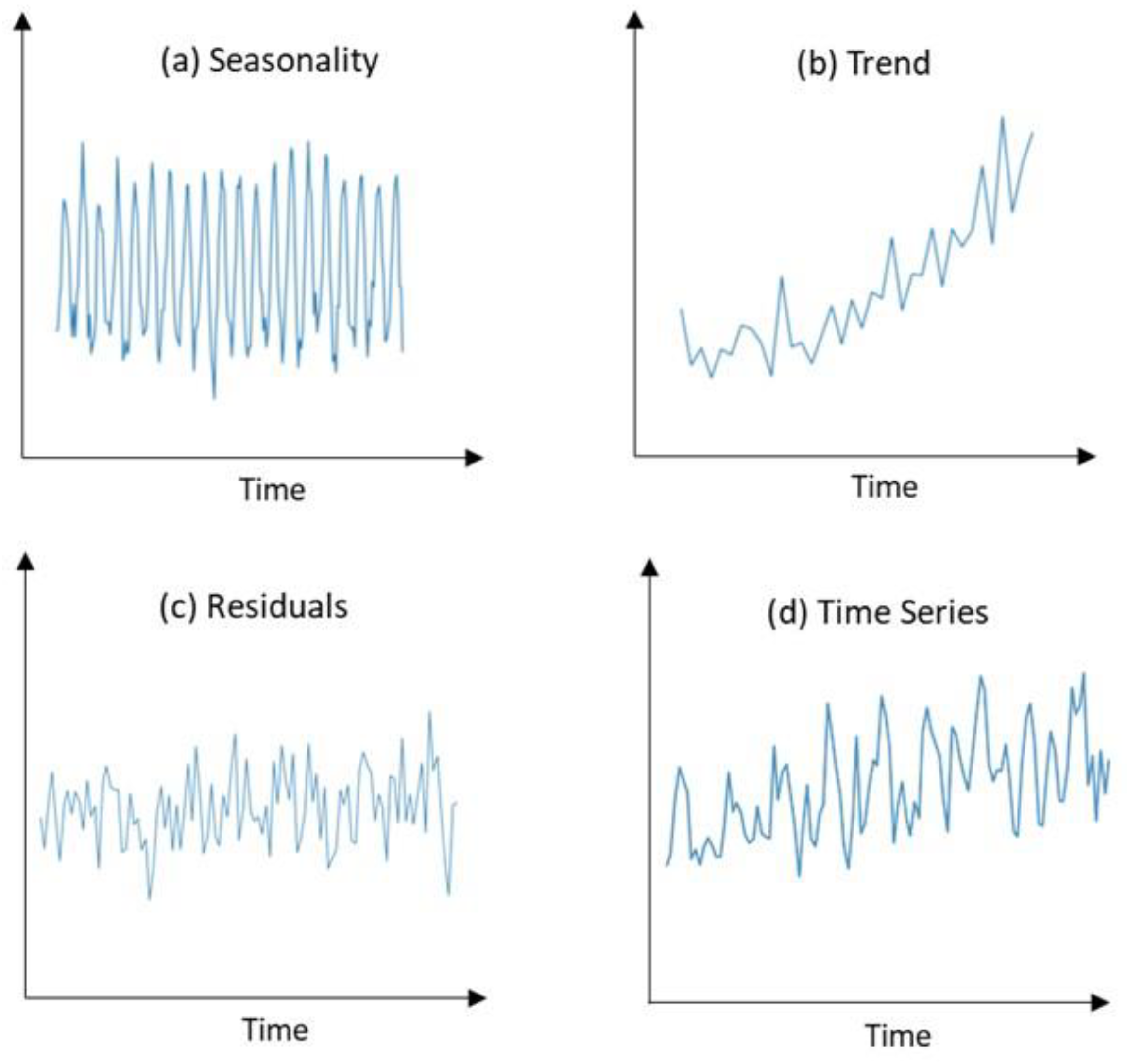
2.1. Time Series

Time-series data are a sequence of observations recorded at regular intervals and arranged chronologically. A time series depicts the temporal development of a dynamic system with the aim of defining, understanding, and forecasting [13]. However, the unique properties of time series data often make the analysis difficult.

Forecasting is used to model the predictors of future time series values by considering past values (lag). Forecasting problems can be categorized as short-, medium-, and long-term based on prediction timeframes [14]. Forecasting techniques can detect, predict, and extrapolate past data trends. The statistical features of historical data are used to foresee patterns and trends to model time series [15].

The time series forecasting problem can be formulated mathematically [16]. Let $X=\left\{x_1,x_2, \dots , x_T\right\}$ be the historical data of a time series, and H be the desired forecasting horizon. The task is to predict the future values of the series $\widehat{X}=\left\{{\widehat{x}}_1,{\widehat{x}}_2, \dots , {\widehat{x}}_T\right\}$. The objective is to reduce the prediction error as follows:

$$E={\displaystyle \sum }_{i=1}^{h=H}\left|x_{T+i}-{\widehat{x}}_{T+i}\right|$$

(1)

Real-world time series include irregular components that are nonstationary, and the mean and variance are not constant over time. The trend, seasonality, residuals, and aggregates of such components are typically used to define a time series (Figure 1). The trend is a general movement; seasonality is periodic fluctuation; and residuals are outliers that obscure the trend and seasonality [17].

However, the presence of these components is not advantageous for accurate forecasting. Therefore, many classical forecasting methods attempt to decompose the time series into three components and independently predict each component. Decomposition is a crucial pre-processing step for extracting nonstationary effects (deterministic components) from a raw time series and capturing the remaining stochastic component [13]. Deterministic components are predictable and contribute to predictions through estimations or extrapolation. The decomposition results in the time series becoming stationary. In a time series analysis, stationarity is an essential and desired attribute. It indicates that the distribution of a variable remains constant across time, which simplifies modeling and forecasting tasks.

The time series may be classified as univariate or multivariate, according to the number of variables at each time step. The univariate time series forecasting problem involves only a single channel and no other variables; therefore, the predictors consist only of sequences of target channel vectors, y. Conversely, the multivariate time series forecasting problem comprises a single target channel, where the predictors are vector pair sequences (x; y) [18].

2.2. Data-Driven Models

The complexity of time series models has increased from classical to modern methods. To determine which model should be used for a particular time series, the model diagnosis and performance metrics must be considered.

2.2.1. Autoregressive (AR)

The prominent classical time series model is autoregressive (AR) with statistical algorithms [19]. AR models an output value based on a linear combination of input values and relies on rolling averages. The input variables (lag variables) are taken as observations at the previous time steps. Using the observations at the current and previous time steps, the value at the next time step can be predicted. The AR process can be described using Equation (2) [18]:

$$Z_t={\displaystyle \sum }_{i=1}^p{\varphi }_i Z_{t-1}+\sigma {ϵ}_t$$

(2)

where ${ϵ}_t$ is a white noises process, p is a hyperparameter to be fixed, $\{{\varphi }_0,{\varphi }_1, \dots , {\varphi }_2,\sigma \}$ are the model parameters, and Z is the response variables. The prediction of autoregressive time series, such as AR(2) given by X(t) = $\alpha$(t − 1) + $\beta$(t − 2) + $\epsilon$(t) ³, may entail highly non-linear functions when sampled irregularly [20]. It is possible to demonstrate the conditional expectations (Equation (3)):

$$\mathbb{E}\left[X\left(t\right)|X\left(t-1\right),X\left(t-k\right),k\right]=a_{k}X\left(t-1\right)+b_{k}X\left(t-k\right)$$

(3)

where $a_k$ and $b_k$ are rational functions of $\alpha$ and ${\beta }^4$. When X is an AR series of higher-order and more past observations are known, the corresponding expectation $\mathbb{E}\left[X\left(t\right)|\left\{X\left(t-m\right),m=1, \dots , M\right\}\right]$ includes more complex functions that generally may not allow closed-form expressions.

The AR technique is often used for stationary time series and linear problems. It is widely used because it can provide valuable statistical features. Additionally, it is highly adaptable because it can represent multiple time series using different order parameters. However, this model is inherently susceptible to the overfitting of long-term temporal trends in long-term temporal patterns [19].

2.2.2. Multilayer Perceptron (MLP)

The multilayer perceptron (MLP) is the most prominent type of artificial neural network (ANN). MLP can be used for time series forecasting for several reasons. First, it is resilient to noise in the input data, and supports learning and prediction when missing values are present. Second, it is nonlinear because it does not make strong assumptions about the mapping function and readily learns linear and non-linear relationships [21]. MLP can also support multivariate and multistep forecasts.

The architecture of an MLP is composed of an input layer, a hidden layer, and an output layer. Each hidden layer has a certain number of neurons to be specified. Each neuron in the hidden layer contains input (x), weight (w), and bias (b) terms. For example, if the MLP structure for the classification problem contains one hidden layer with sigmoid and softmax as activation functions, then the feedforward computation is described by Equation (4):

$$y_i=softmax\left(\sigma \left(xW+b\right)V+c\right)$$

(4)

where y_i is the prediction, $\sigma$ is the sigmoid function, W is the weight between the input and hidden layers, V is the weight between the hidden and output layers, x is a feature, b is the bias between the input and hidden layers, and c is the bias between the hidden and output layers.

Backpropagation is used to determine the gradient of the cost function (J) during the learning phase. The error in the output layer propagated back to the preceding layers. The weights were computed by minimizing the cost function, as indicated in Equation (5), utilizing gradient descent optimization methods.

$$\frac{\partial J}{\partial W}={\displaystyle \sum }_n{\displaystyle \sum }_k\left(t_{nk}-y_{nk}\right)z_{nm} V_{mk}{z}_{nm}\left(1-z_{nm}\right)x_{nd}; \frac{\partial J}{\partial V}={\displaystyle \sum }_n\left(t_{nk}-y_{nk}\right)z_{nm}$$

(5)

where t is the target, y is the output in the output layer, z is the output in the hidden layer, the subscript n is a sample, k is the class, m is the hidden layer, and d is the input layer.

2.2.3. Long Short-Term Memory (LSTM) Network

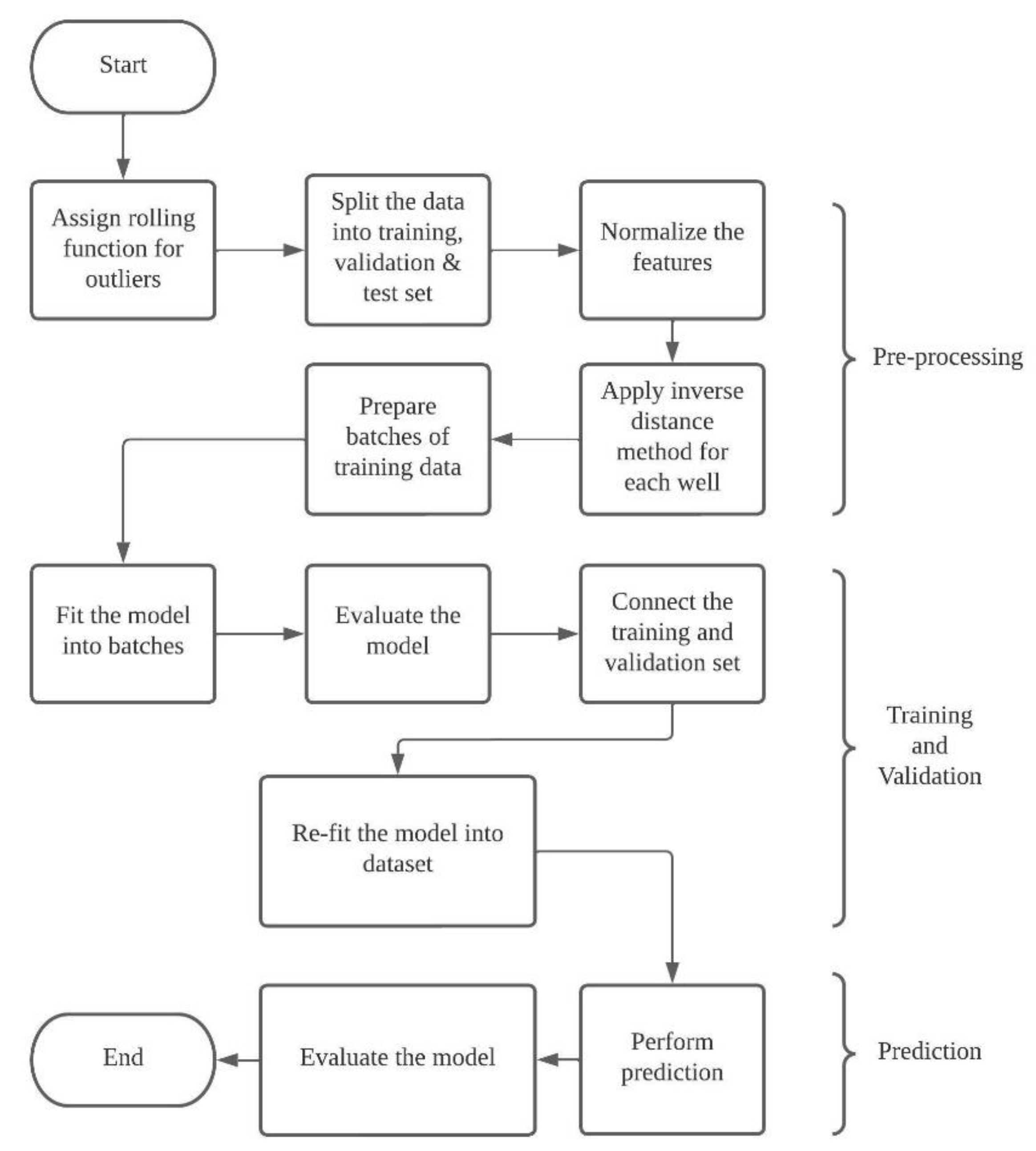
The LSTM network is a model that extends the recurrent neural network (RNN) memory and may assist in resolving short- and long-term dependencies, thereby simplifying the recall of past data. As a model, it saves knowledge learned in a short time and employs it for long-term training. In addition, LSTM provides native support for inputting sequence data and can overcome vanishing gradients [22]. Therefore, LSTM models are primarily used for the time series data.

Traditional neural networks consist of neurons, whereas LSTM networks are composed of memory blocks connected through consecutive hidden layers. There are three types of gates in a memory block: input, forget, and output. Depending on the sigmoid activation function, the gate may be activated. This function enables the network to determine hidden states that it must forget and refresh.

The feedforward calculation of the LSTM is shown in Equations (6)–(10) [23]:

$$f_t={\sigma }_g\left(W_f{x}_t+U_f{h}_{t-1}+b_f\right)$$

(6)

$$i_t={\sigma }_g\left(W_i{x}_t+U_i{h}_{t-1}+b_i\right)$$

(7)

$$o_t={\sigma }_g\left(W_o{x}_t+U_o{h}_{t-1}+b_o\right)$$

(8)

$$c_t=f_t\ast c_t+i_t\ast {\sigma }_c\left(W_c{x}_t+U_c{h}_{t-1}+b_c\right)$$

(9)

$$h_t=o_t\ast {\sigma }_h\left(c_t\right)$$

(10)

where $x_t$: input vector to the LSTM; $f_t$: forget gate activation vector; $i_t$: input gate activation vector; $o_t$: output gate activation vector; $h_t$: output vector of the LSTM unit; $c_t$: cell state vector; ${\sigma }_g$: sigmoid function; ${\sigma }_c, {\sigma }_h$: hyperbolic tangent function; W, U: weight matrices that needs to be learned; and b: bias vector parameter that needs to be learned. Backpropagation through time is used to train the LSTM networks, which helps avoid the vanishing gradient problem.

3. Methods

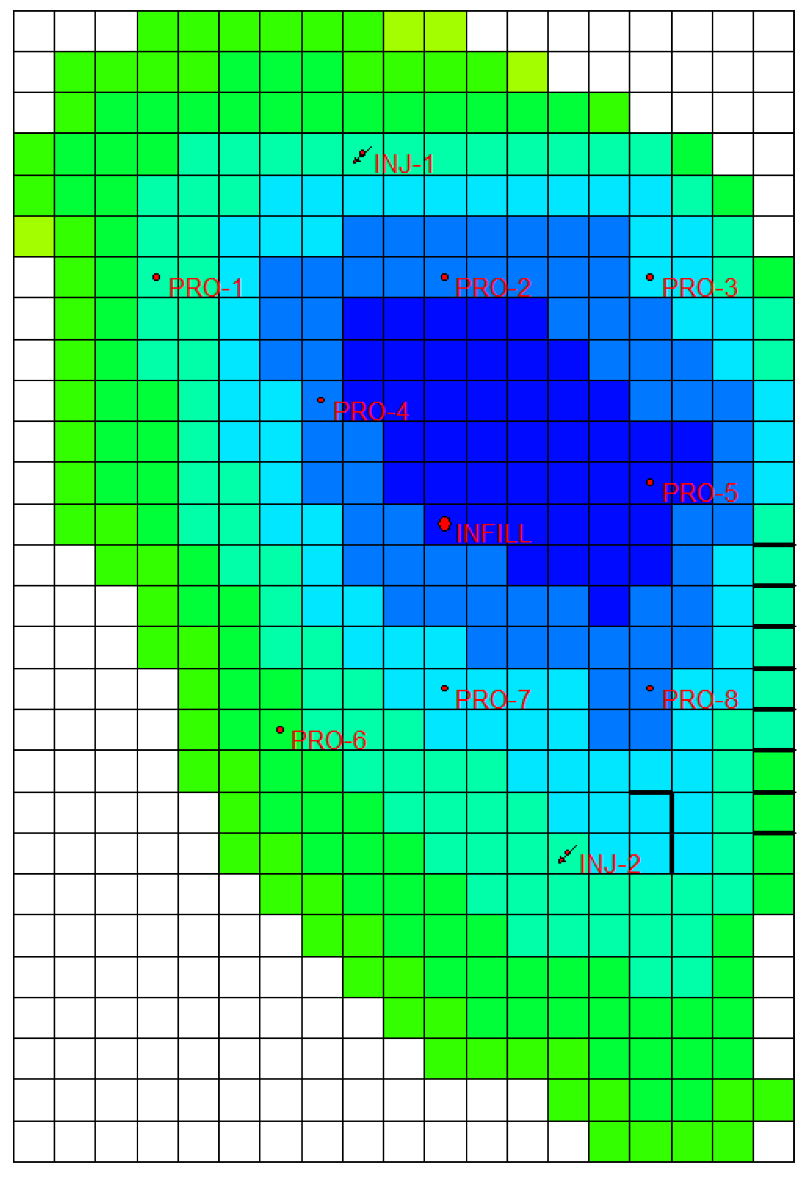
3.1. Reservoir Model

To create a data-driven reservoir model for simulating the CO₂-EOR and CO₂ storage processes, a PUNQ-S3 model was employed to produce a dataset encompassing production-influencing features as the input and the corresponding fluid production as the output. Ideally, the data required to construct a model should be acquired from the field. However, when actual data are not accessible, this dataset may alternatively be generated using numerical or analytical models [24].

The PUNQ-S3 reservoir model is synthetic; however, it exemplifies a representative geological model for flow simulations and has been used in various reservoir simulation studies [25,26]. The five-layer reservoir model is qualified as a small industrial reservoir engineering model containing 19 × 28 × 5 grid blocks, of which 1761 blocks are active. The grid blocks have equal 180 m sides in the x- and y-directions. The properties of the PUNQ-S3 reservoir model are summarized in

Table 1. Parameters of the PUNQ-S3 model.

Parameter	Value	Unit
Pressure at reference depth	28,300	kPa
Bottomhole flowing pressure	19,810	kPa
Pressure Fracture	42,450	kPa
Reservoir temperature at reference depth	110	°C
Free water level	2395	m
Free oil level	2355	m
Initial water saturation	0.2	fraction
Initial oil saturation (oil zone)	0.8	fraction
Initial oil saturation (gas cap)	0.3	fraction
Initial gas saturation (gas cap)	0.5	fraction
Reference depth	2355	m

.

The well configurations implemented on PUNSQ-S3 are shown in Figure 2. Each of the eight producing wells (PRO-1 to PRO-8) was placed with permeability distributions on each layer as guidance. Consequently, each well has several components in the productive layers (

Table 2. Completions for each well.

	Perforated Layer
Well	1	3	5
PRO-1		●
PRO-2			●
PRO-3	●	●	●
PRO-4			●
PRO-5		●	●
PRO-6	●	●	●
PRO-7	●	●	●
PRO-8	●		●
INFILL	●

) so that they may contribute to oil production. Additionally, two CO₂ injection wells (INJ-1 and INJ-2) were positioned in the northern and southern parts of the reservoir to sweep the remaining residual oil.

The production scheme began with a natural depletion over five years. Afterward, 10 years of continuous miscible CO₂ injection was conducted with an injection pressure and rate of 32,545 kPa and 7000 m³/day, respectively. Finally, the infill well was planned to be drilled 10 years after CO₂ injection.

3.2. Data

The forecasting models were developed using a dataset comprising production data from eight wells (PRO-1 to PRO-8). A total of 3653 observations were recorded over 10 years, from January 2004 to December 2013. The dataset was generated from numerical simulation results with the PUNQ-S3 model. It was assumed as raw or actual data from field measurements for constructing the data-driven models. The field dataset was assumed to be composed of daily records of the time series data of a well. Generally, the time intervals between data points may be diverse. The time series data included oil production (m³/day), water production (m³/day), and gas production (CO₂-kg/day) (Figure 3, Figure 4 and Figure 5). These data were measured using multiphase flow meters at the producing wells in the field.

3.2.1. Features

Six parameters affecting fluid production were selected as features to build the data-driven models. Besides that, these parameters were selected due to the following reasons: (i) they are readily available from field measurements and do not require processing and acquisition from the lab; (ii) they represent the capability of the well to produce a fluid; (iii) each well has its unique values which help to distinguish the characteristics between wells: as a result, the data-driven model can learn and correlate the selected parameters to production characteristics of each well.

These parameters were divided into static parameters: porosity, permeability (mD), formation thickness (m), well location x-axis (i), and well location y-axis (j), and dynamic parameters: bottom hole pressure (BHP-kPa) (

Table 3. Features for building a data-driven model.

Well	Avg. Porosity	Avg. Permeability (mD)	Storage Capacity (m)	Flow Capacity (mD-m)	Avg. Fm Thickness (m)	BHP (kPa)	i	j
PRO-1	0.43	988.0	1.462	3359.2	3.40	20,500	4	22
PRO-2	0.43	804.0	1.634	3055.2	3.80	19,100	11	22
PRO-3	0.43	690.3	1.658	2551.9	3.90	20,000	16	22
PRO-4	0.42	963.0	1.932	4429.8	4.60	18,700	8	19
PRO-5	0.32	370.0	1.632	1887.0	5.10	19,800	16	17
PRO-6	0.40	897.7	1.956	4375.6	4.93	20,800	7	11
PRO-7	0.34	536.0	1.298	1961.8	3.97	20,100	11	12
PRO-8	0.24	370.0	0.784	1231.7	3.65	19,500	16	12
INFILL	0.41	906.0	2.132	4711.2	5.2	20,000	11	16

). The first five features are (fixed) reservoir properties, whereas the sixth feature is an operational constraint that can be controlled during production. Because certain wells were completed in several layers, features such as porosity and permeability could not be simply averaged without considering the thickness of each layer. Such features were engineered at a storage capacity and flow capacity that represented a better quantitative relationship between the reservoir properties and production data.

3.2.2. Preprocessing

Reservoir production time series may include anomalies and incorrect observations due to unanticipated occurrences, flawed measurements, and human interference. These anomalies may modify the series, making it challenging for the forecasting model to discover prediction patterns. Therefore, data pre-processing is required to eliminate outliers, complete the missing data, and transform the data. Because the data were generated by simulation, treating the missing data was unnecessary. However, outliers were removed from the numerical noise owing to the difficulty of achieving convergence of the simulation. A rolling function is used to address these outliers.

Next, the data were normalized for further analysis. Data normalization is standard in data-driven techniques because of the varying dimensions and units of input data. Normalization of data expedites the convergence of models and reduces the training errors. Min–max normalization is a general and effective procedure [27]. This process is represented as follows:

$$x_{new}=\frac{x_{old}-x_{min}}{x_{max}-x_{min}}$$

(11)

where $x_{new}$: new feature value; $x_{old}$: old feature value; $x_{max}$: maximum feature value; and $x_{min}$: minimum feature value.

3.2.3. Exploratory Data Analysis (EDA)

Data exploration techniques have been applied to discover hidden insights from the dataset [14]. Visualization of a dataset was performed to determine the trends and seasonality patterns in the data without transforming or altering the dataset. Notably, this should be the first step before beginning the time series modeling.

As shown in Figure 3, Figure 4 and Figure 5, the production data by day, month, and year do not show seasonal fluctuations, cycles, or oscillation amplitude and lack a discernible pattern. This indicates that the production data are stationary and resemble a typical stationary form, as depicted in Figure 6. Therefore, it is unnecessary to transform the data into a stationary format.

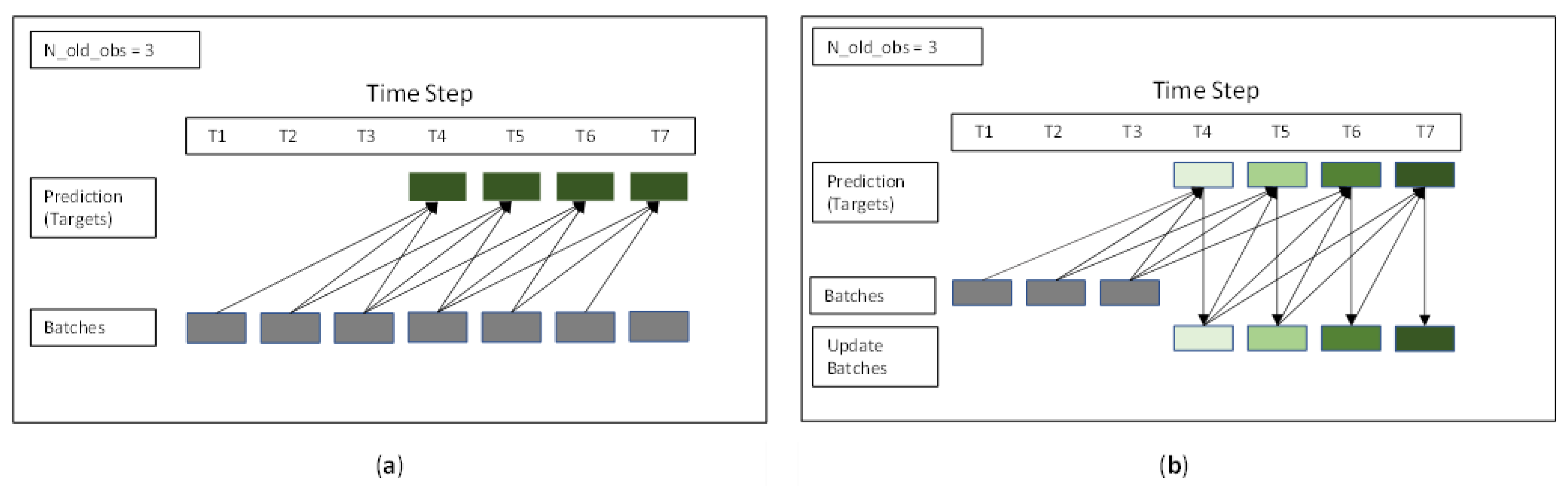
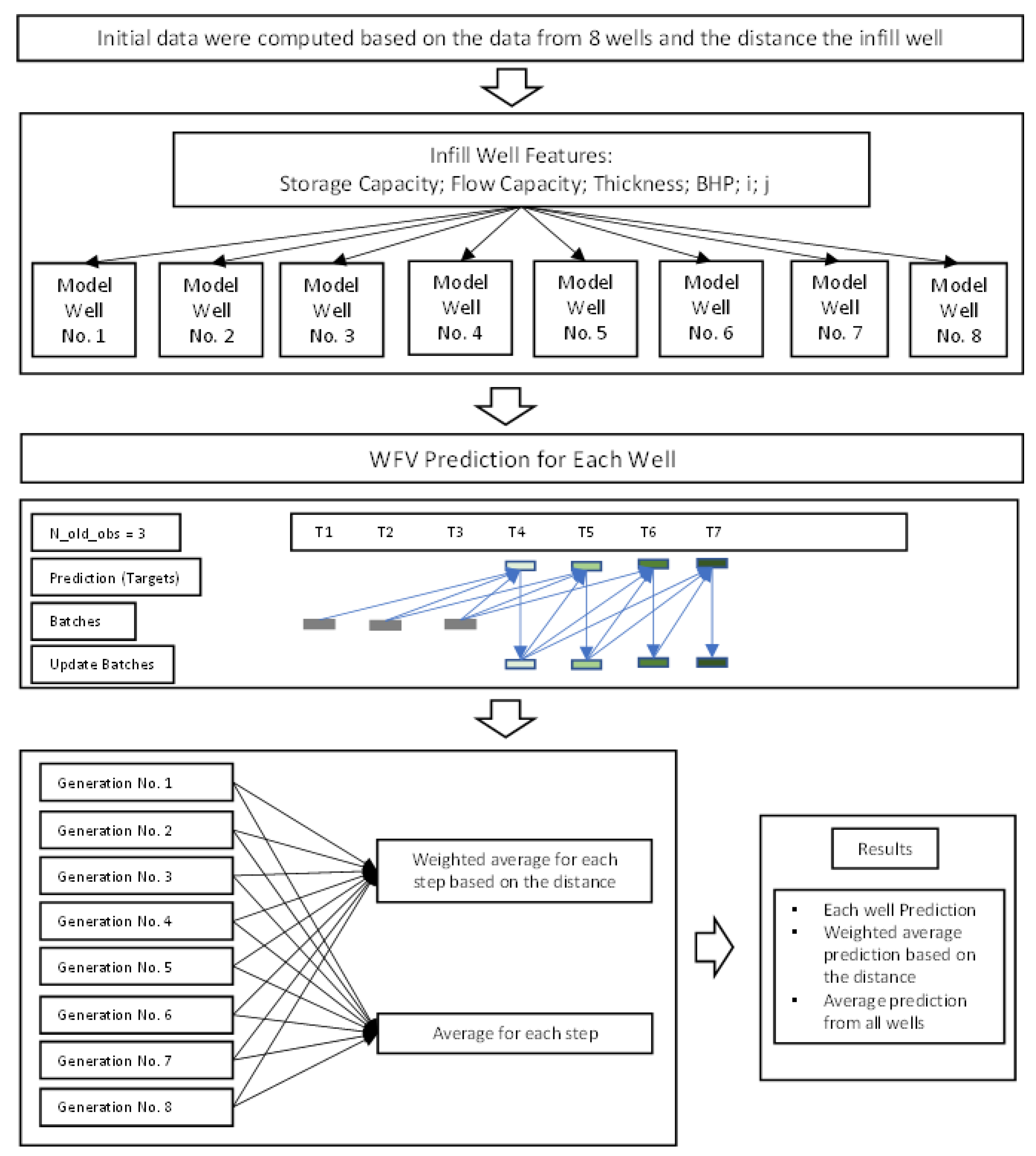
3.3. Problem Formulation

Injecting fluid into a reservoir causes a pressure pulse, which takes some time to reach the production wells due to diffusivity [28]. The connectivity among the wells must be factored in to teach the data-driven model the concepts of fluid displacement, pressure interference between wells, and the impact of operational constraints and reservoir characteristics on production. By combining data from several wells, the model captures the field behavior caused by the interference between the surrounding wells at different rates. This phenomenon was modeled by correlating the flow rate at each well and at each time step to a set of static and dynamic parameters proportional to the well distance. Physical phenomena such as the volume expansion of crude oil, mixing phases, phase transition of oil–gas mixtures, CO₂ dissolution in the fluid, interface tension between water and oil, etc., are implicitly captured by the model and represented by the data. In contrast, in traditional reservoir modeling, such physics are represented by theoretical/empirical equations.

The inverse distance method [29] was used to account for the interference surrounding the wells (Equations (12)–(14)):

$$D_{A-B}=\sqrt{{\left(i_A-i_B\right)}^2+{\left(j_A-j_B\right)}^2}$$

(12)

$$W_{A-B}=\frac{1}{{\left(D_{A-B}\right)}^f}$$

(13)

$$Weighted Flui{d}_{A\left(o,w,g\right)}=W_{A-B}\times Flui{d}_{A\left(o,w,g\right)}$$

(14)

where D_A−B: Distance from Well-A to Well-B, W_A−B: Weight of Well-A–Well-B, f: factor for inverse distance, and (i,j): well location.

This notion was formulated as a multivariate time series forecasting problem in which the architecture of the data-driven model is sequence-to-vector (Seq2Vector). Two different data-driven models were tested: global and reduced feature models. The global model was trained on a dataset composed of measurements from multiple wells by considering the 3-phase flow (oil, water, and gas). Similarly, the reduced feature model was trained on the dataset composed of measurements from multiple wells but with one phase at a time. The input and output with three old observations (N_old_obs = 3) for the global and reduced feature models are shown in Figure 7 and Figure 8, respectively.

The time series was sliced into samples of N lengths of old observations (N_old_obs) using the sliding window technique. The sliding window was used to transform the forecasting problem into a regression task, capture nonlinear relationships, and add memory to the problem for contextual prediction [13]. It also allows the model to capture the autocorrelation effect of the target variable. Defining the window size (time lag) is difficult because there is no assurance that adequate information is acquired. However, this parameter will be tuned along with other hyperparameters.

The implementation was conducted by dividing the features into the following subgroups: Constants [BHP, FM Thickness, Permeability, Porosity]; Variables [Oil, Water, Gas productions]; Coordinates [i, j]; and Gradients [gOil, gGas, gWater]. Gradients are the difference between each production data observation, which better indicate the curvature. The data were prepared in batches for each model in a high-dimensional tensor.

Before the data were fed into the model, they were flattened to form one input instance. For example, for N_old_obs = 3, the input and target shapes for each data-driven model were as follows:

$$\begin{array}{c}Input=\left[1, \left(3\_var+3\_grad\right)\ast 3\_n\_old\_obs\ast 8\_wells+4\_cons+2\_coor\right]=\left[1, 150\right]\\ Target \left(AR\right)=\left[1,3\right]\\ Target \left(MLP and LSTM\right)=\left[1,1\right]\ast 3\end{array}$$

where var: variables (oil, gas, water); grad: gradients (oil, gas, water); cons: constants, coor: coordinates. Only for AR did the model simultaneously generate three outputs once.

3.4. Model Development

Data-driven models were developed using the Keras framework with the backend TensorFlow. The development stage is illustrated in Figure 9. Unlike cross-sectional data, time series data cannot be randomly subdivided because the sequential information within a set must be preserved. Therefore, the last segment of the series was used as the test set, the second segment as the validation set, and the first segment as the training set. These segments consisted of training (40%, 4 years), validation (20%, 2 years), and test sets (40%, 4 years). Fifty epochs were used to train the models. A validation set was used to configure the data-driven model’s hyperparameters. Once the hyperparameters of the model were optimized, the model was retrained using a new dataset combining the training and validation sets. The validation set may contain pertinent information for providing future forecasts. Finally, the generalization capability of the overall model was evaluated using the test set.

3.5. Model Evaluation and Prediction

For forecasting problems, the typical approach to evaluating a model is to determine the error between the actual value and the prediction value. The mean absolute percentage error (MAPE), as given in Equation (15), was used as the performance metric. The MAPE is convenient for this case because the error values are presented as percentages. Although the root mean square error (RMSE: Equation (16)) is often employed, the datasets comprise distinct time series with different units, making it impossible to directly evaluate the accuracy of different time series datasets.

$$\mathrm{MAPE}=\frac{1}{n}{\displaystyle \sum }_{i=1}^n\left(\frac{\left|{\widehat{y}}_i-y_i\right|}{y_i}\right)\times 100\%$$

(15)

$$\mathrm{RMSE}=\sqrt{\frac{{{\displaystyle \sum }}_{i=1}^n{\left({\widehat{y}}_i-y_i\right)}^2}{n}}$$

(16)

k-fold cross-validation is the gold standard for data-driven evaluation methods. However, this method cannot be used for time series data for various reasons: (i) it assumes that there are no dependencies between the observations, and (ii) it splits the data into groups at random. These are not true for time series because each observation is dependent, and the temporal order should be honored.

Backtesting/hindtesting is a standard method for evaluating time series models using past data. There are several backtesting methods, such as train–test split with respect to the temporal order of observations, multiple train–test splits that respect the temporal order of observations, and walk-forward validation (WFV). The WFV method was adopted to evaluate the model on the validation set and to perform predictions on the test set. However, the model was not updated during the WFV process. WFV methods were used for prediction, particularly WFV over data and WFV. The WFV over data method uses actual observations of the current period to predict subsequent periods. This method predicts a one-time step (T + 1) for oil, gas, and water production.

In contrast, WFV uses only the last number of actual observations to make the next prediction. Once the last observation is used, the model uses observations generated by the model in the previous time step. Thus, WFV can perform multistep predictions. In other words, the WFV method generates forecasts for T time steps simultaneously, whereas the WFV over data generates forecasts in a rolling fashion (Figure 10).

Predictions for the infill well performances were also made using a similar methodology. The future time series for the infill well was derived using the knowledge from eight existing wells (Figure 11). Each well represents a data-driven model with unique features. WFV prediction was employed using the last segment of observations of the time series data of existing wells, and they were weighted proportionally to the distance of the infill well. Subsequently, the infill well’s features were fed into the existing wells. In addition to generating the prediction from an individual well, the predictions were also made by weighted averaging and simple averaging the time series data of existing wells.

The curvature shape generated from the trained model of the existing wells was evaluated based on the shape of the actual data. The process involves normalizing the generated curve using Equation (17):

$$Scor{e}_{shape}=\frac{{{\displaystyle \sum }}_{i=1}^n\left|y{\left(norm\right)}_i-\widehat{y}{\left(norm\right)}_i\right|}{n}$$

(17)

where y: target, $\widehat{y}$: prediction result, and n: number of samples.

3.6. Model Optimization

Data-driven model optimization is essential to the speed of training and forecast precision. The model is optimized by determining its hyperparameters according to prediction performance. The search strategy employed to optimize the model is a grid search. The grid method explores the potential combinations for a set of predetermined hyperparameters.

Table 4. Hyperparameters of data-driven models for tuning.

Hyperparameters	Data Driven Model	Description	Range
Hidden layers	MLP/LSTM	It determines the depth of the neural network.	[4, 5, 6, 7, 8]
Dropout	MLP/LSTM	It eliminates certain connections between neurons in each iteration. It is used to prevent overfitting.	[0.01, 0.001, 0.0001]
L1/L2 Regularization	MLP/LSTM	It prevents overfitting, stopping weights that are too high so that the model does not depend on a single feature.	[0.0001, 0.00001, 0.000001, 0.0000001, 0.00000001]
Units	MLP/LSTM	It determines the level of knowledge that is extracted by each layer. It is highly dependent on the size of the data used.	[128, 256, 512, 1024]
N_old_obs	AR	The number of observations used for the model.	[15, 20, 25, 30]
Mod_update	AR	The number of observations after which the updated model should be generated.	[25, 50, 100, 200, 400]
W_model_init	AR	The ratio for the initial model to the updated model to be taken into consideration.	[0.00, 0.5, 1.00]

summarizes, based on early tests, the ranges of feasible values and pertinent hyperparameters [17]. This process was applied to both global and reduced feature models.

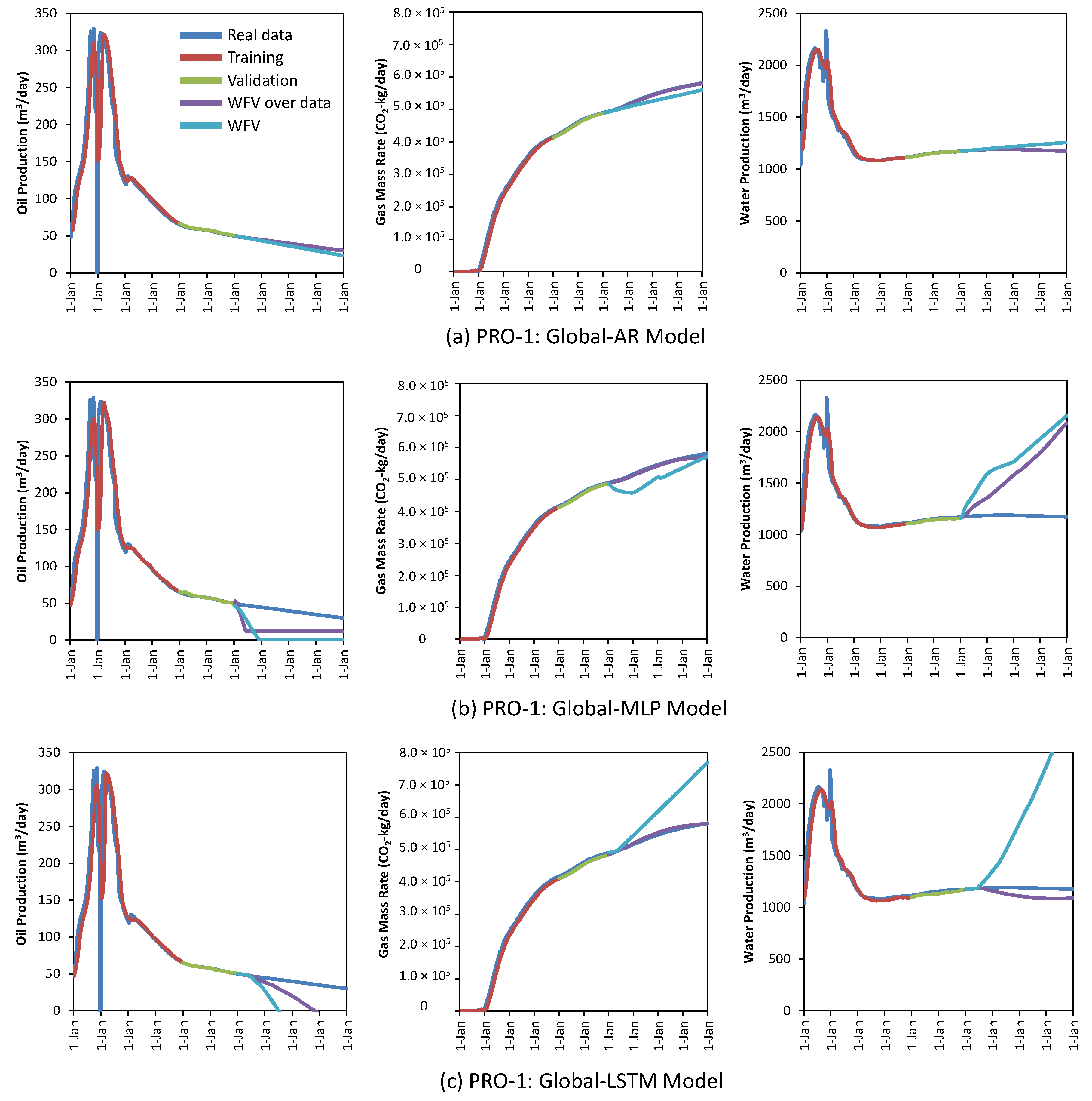
4. Results and Discussions

4.1. Model Optimization

As the number of hidden layers and neurons increases in deep learning, neural networks provide power and flexibility, leading to improved accuracy [30]. However, this is not always the case, because different problems require different configurations. Therefore, experiments with different topologies are required.

Table 5. Results of topology and hyperparameters tuning.

Model	Parameter	Global Model	Reduced Feature Model
			Oil	Gas	Water
AR	Factor for inverse distance	20	20	20	20
	Number of previous observations	30	30	30	25
	Optimizers	Least square	Least square	Least square	Least square
	Ratio for initial/update model	0.0:1.0	0.0:1.0	1.0:0.0	0.0:1.0
	No. of observations to update model	50	25	200	25
MLP	Factor for inverse distance	20	20	20	20
	Number of previous observations	5	5	5	5
	Optimizers	Adam	Adam	Adam	Adam
	Activation function	ReLU	ReLU	ReLU	ReLU
	No. of hidden layers	8	8	4	8
	No. of units	1024	512	1024	256
	Dropout	0.01	0.01	0.0001	0.0001
	Kernel regularizator	L1	L1	L1	L1
	Kernel regularizator rate	0.000001	0.00000001	0.0000001	0.0000001
	Activity regularizator	L2	L2	L2	L2
	Activity regularizator rate	0.00001	0.0001	0.0000001	0.00001
LSTM	Factor for inverse distance	20	20	20	20
	Number of previous observations	5	5	5	5
	Optimizers	Adam	Adam	Adam	Adam
	Activation function	ReLU	ReLU	ReLU	ReLU
	No. of hidden layers	6	7	8	8
	No. of units	1024	256	512	512
	Dropout	0.01	0.001	0.0001	0.001
	Kernel regularizator	L1	L1	L1	L1
	Kernel regularizator rate	0.0001	0.0001	0.0000001	0.000001
	Activity regularizator	L2	L2	L2	L2
	Activity regularizator rate	0.00000001	0.0000001	0.0000001	0.000001

displays the results of the topology adjustment and hyperparameter optimization for the AR, MLP, and LSTM models.

Overfitting occurred during training. Therefore, dropout was introduced to enhance the generalization capability of the model. This strategy reduces overfitting by randomly selecting neurons to be ignored during training with a given probability. The selected neurons are temporarily omitted from the feedforward computation. Therefore, the network becomes less sensitive to the specific weights of neurons, which forces the network to distribute its learning.

Optimizing N_old_obs, Mod_update, and W_model_init for the AR model improved its prediction capability. The AR model is particularly sensitive to the number of observations used for the model (N_old_obs) and the number of observations required to update the model (Mod_update).

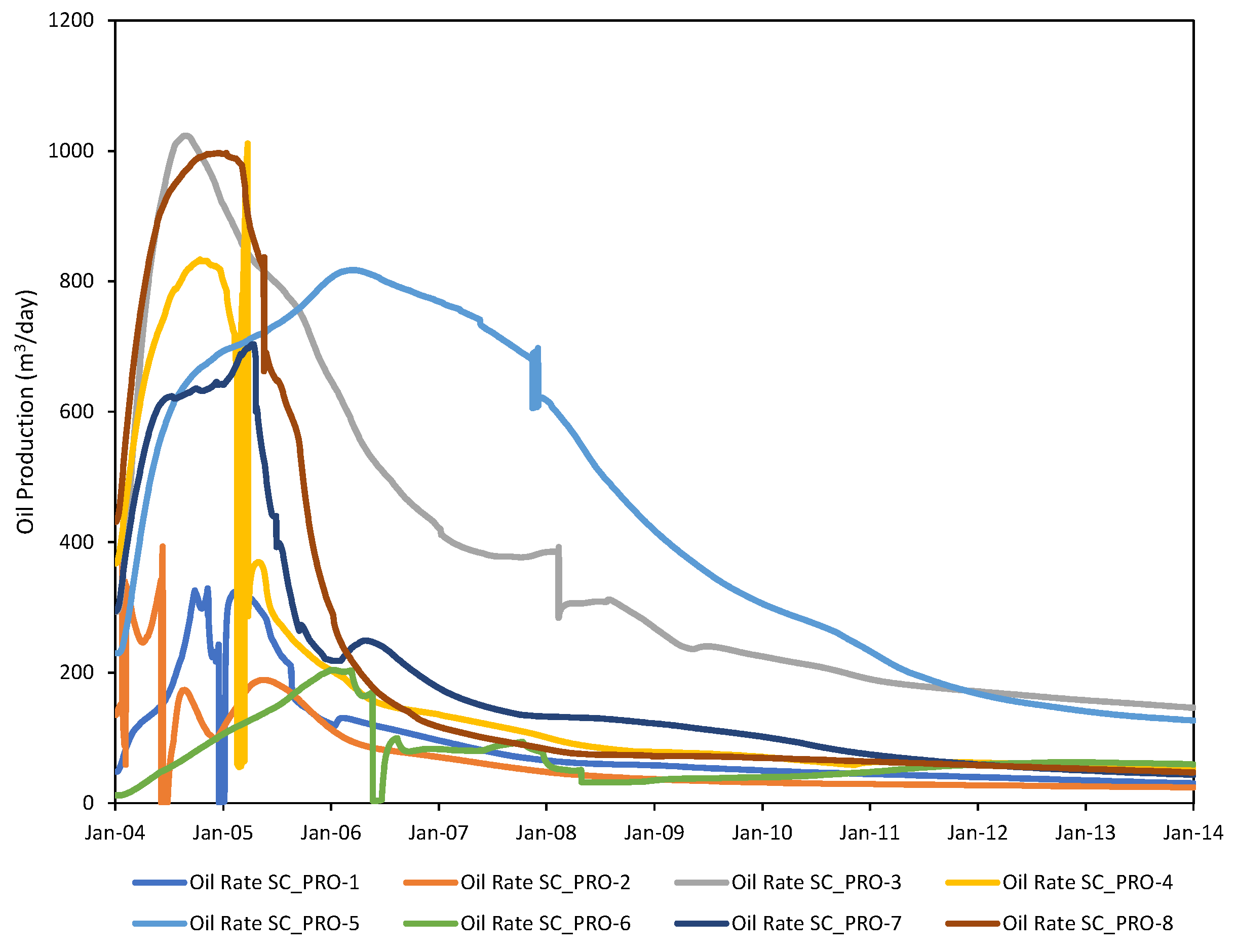
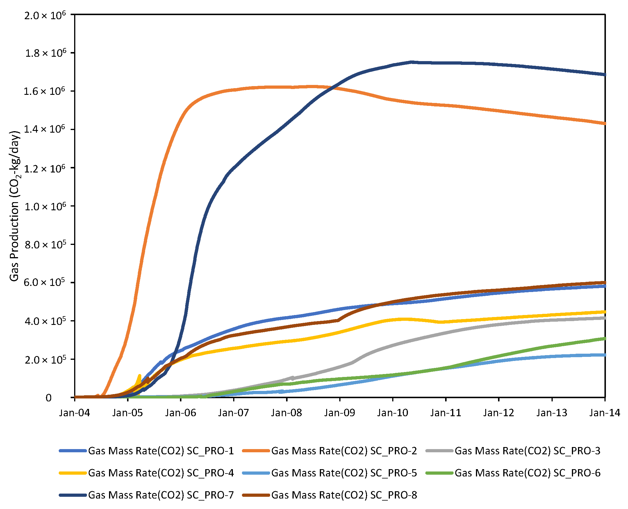
4.2. Existing Well Prediction

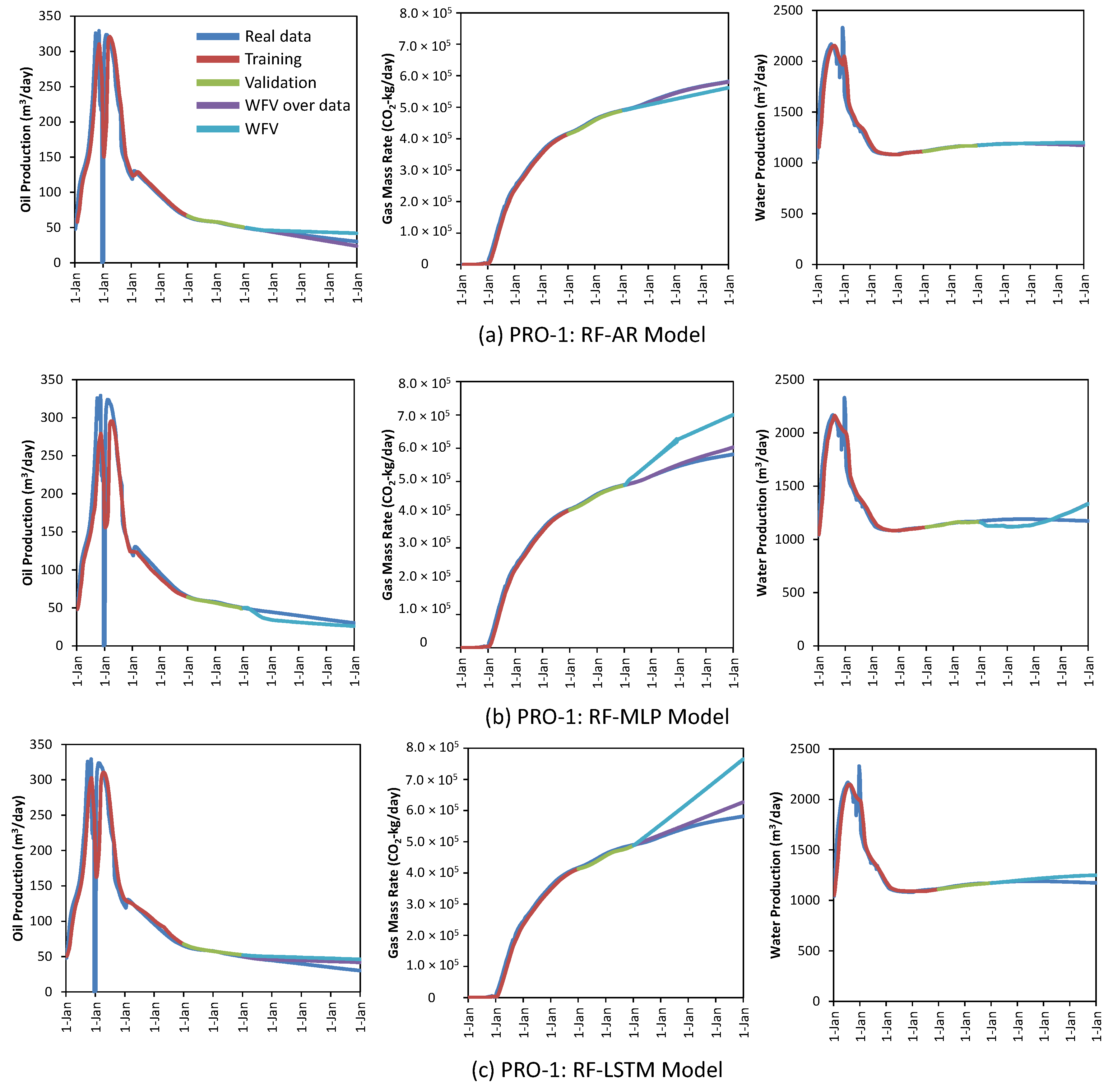
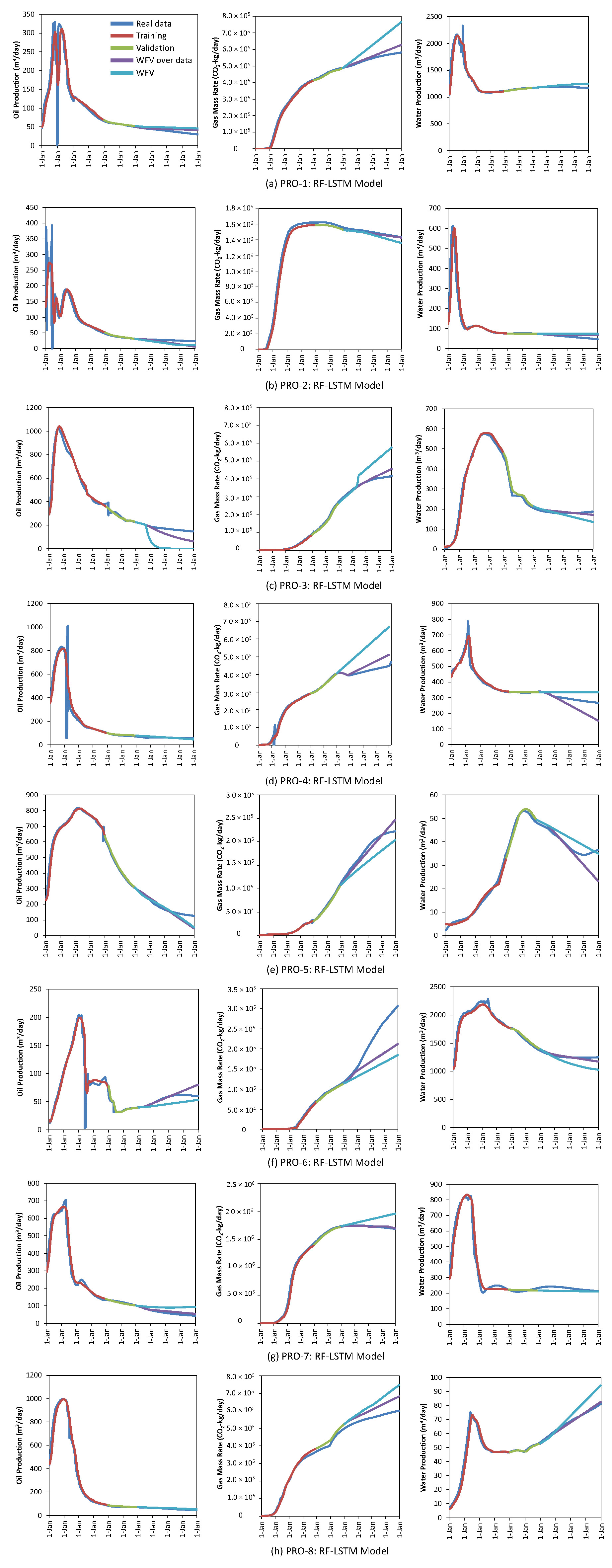
4.2.1. Global Model

The global model forecasts the values of the time-dependent target parameters based on the inverse distance and the 3-phase flow of oil, gas, and water from each well to the target well. This accounts for the effect (interference) of wells on each other throughout the injection and production processes. The predictive performance was evaluated based on the test dataset with 1460 observations. Figure 12 illustrates the forecasts of the global models, for AR, MLP, and LSTM with time series data and oil, gas, and water production. Owing to space constraints, only PRO-1 well is shown.

As illustrated by the purple line, the WFV over data predictions (one time step) for the AR model followed the actual data trend until the end of the project for the entire time series. A similar prediction trend was only observed for gas production for the MLP and LSTM models. For every time series, the LSTM model retained the prediction trends for only a certain number of time steps, but the MLP exhibited a significant premature deviation from the actual data.

Access to forecasts at several time steps is often advantageous. This would enable decision makers to see future trends and optimize their actions throughout the course. Such multi-time step forecasts are represented by the light blue lines (WFV) in the graphs. Generally, all models started to deviate from the real data after certain time steps. However, the long-term forecasting horizon of the AR model is more prominent than that of the other models. In contrast, the MLP model deviated far sooner in the majority of the three time series compared with the other models. It struggles to forecast downward slopes for oil production, upward trends, and plateaus for water production. Meanwhile, the LSTM model demonstrates the capacity to follow the trends, although with a shorter forecasting horizon than the AR model.

WFV prediction generally resulted in straight lines in the AR model. This may be due to the fact that AR relies on a linear function. In contrast, the prediction trends for the AR and LSTM models were not linear, owing to the non-linear nature of these models. The deviation shown by the WF prediction can be solved by updating the model after incorporating new data to apply the most recent trend characteristics.

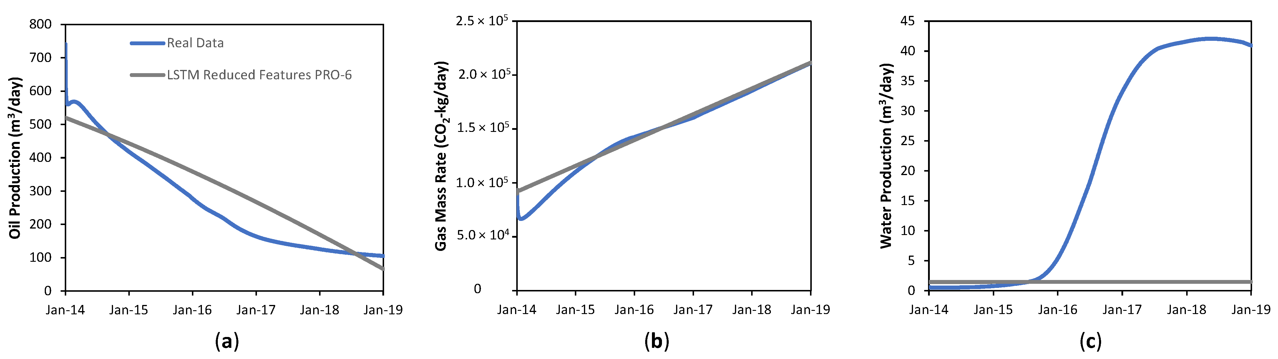
4.2.2. Reduced Feature Model

The input features for the reduced feature model are similar to those of the global model, except that they only consider the flow of particular fluid (oil, gas, or water) or one time series at a time. The forecasting results for all the model types are shown in Figure 13. The AR model continues to forecast over the long-term horizon: either WFV over the data or WFV predictions. The reduction in features in the LSTM model demonstrated a longer forecasting horizon compared to the LSTM global model for both prediction methods. The reproduction of the oil and water trends showed notable improvements. By contrast, reducing the number of features in an MLP model has a minor influence on its predictive power. In general, it is challenging for all models to anticipate an increasing trend in gas prediction, particularly with WFV prediction.

4.2.3. Comparing Global Model vs. Reduced Feature Model

Table 6. Average MAPE of eight wells for all models and predictions.

	WFV over Data			WFV
Model	Oil Rate	Gas Mass Rate (CO2)	Water Rate	Oil Rate	Gas Mass Rate (CO2)	Water Rate
AR—Global	1.16%	0.68%	1.80%	13.37%	9.93%	14.13%
AR—Reduced Feature	1.88%	0.58%	0.50%	15.20%	8.13%	11.67%
MLP—Global	133.60%	6.95%	75.19%	95.60%	16.23%	104.47%
MLP—Reduced Feature	34.59%	5.54%	38.51%	33.47%	15.15%	38.78%
LSTM—Global	41.46%	3.86%	31.25%	142.96%	15.38%	72.19%
LSTM—Reduced Feature	14.84%	5.63%	7.15%	28.87%	12.06%	10.05%

presents the average MAPE values for eight wells for the global and reduced feature models for all model types. These MAPE values were computed over a period of four years. The AR generalization performance across various time series datasets was compelling. It outperformed the other models for both WFV over data and WFV predictions. The reduction in features does not have a major impact on accuracy. As the number of features decreases, the input sequence becomes shorter. Consequently, regardless of the length of the window-based input in the AR model, the model is still able to comprehend the underlying time series structure of the data. This is coupled with the fact that the prediction was made at the tail of the dataset, where the production profile was less variable.

As shown in Table 6, reducing the number of features improved the predictive performance of the MLP and LSTM models for WFV over data and WFV predictions. This was observed in the vast majority of the time series datasets.

Models that were fully augmented generally had worse performance compared to reduced feature models. Particularly for LSTM, a very long input sequence makes it difficult to capture the long-term multivariate dependencies of data for the desired forecasting accuracy for a given dataset [31]. Although MLP is widely recognized as the top performing predictor class in the machine learning industry, with the capacity to map complicated nonlinear feature interactions in a variety of application areas, its intrinsic structure is not designed to handle multivariate long input sequences. From the perspective of the dataset, the time series are neither strongly fluctuating nor characterized by intricate patterns. Such deep learning models may be excessively complicated compared to conventional approaches, in this case AR, when using the same dataset. Additional training data may be required to correlate static and dynamic features for long-term forecasting horizons [13].

Table 7. Average number of days with prediction error <5% for eight wells.

	WFV over Data (Days)			WFV (Days)
Model	Oil Rate	Gas Mass Rate (CO2)	Water Rate	Oil Rate	Gas Mass Rate (CO2)	Water Rate
AR—Global	1430	1430	1343	918	378	856
AR—Reduced Feature	1430	1430	1435	860	452	633
MLP—Global	346	333	84	346	13	83
MLP—Reduced Feature	209	425	30	150	44	18
LSTM—Global	180	269	261	158	177	172
LSTM—Reduced Feature	269	284	278	176	187	183

presents the average number of days for each prediction method, with an error of less than 5%. For the WFV over data and WFV prediction methods, both the AR global and reduced feature models are capable of long forecasting horizons of at least one year. Conversely, the MLP and LSTM models have shorter forecasting horizons than the AR model does. The shortest forecasting horizon for MLP is 13 days for gas production, whereas LSTM has a minimum of 5 months for oil production.

These numbers represent the means of the eight wells for each model type and prediction method. To evaluate the consistency of the model forecasts,

Table 8. Standard deviation of average number of days with prediction error <5% for eight wells.

	WFV over Data (Days)			WFV (Days)
Model	Oil Rate	Gas Mass Rate (CO2)	Water Rate	Oil Rate	Gas Mass Rate (CO2)	Water Rate
AR—Global	0	0	0	424	242	503
AR—Reduced Feature	0	0	243	442	260	495
MLP—Global	253	466	39	184	53	26
MLP—Reduced Feature	518	457	210	518	12	211
LSTM—Global	12	10	11	13	12	12
LSTM—Reduced Feature	7	9	9	13	11	15

shows the standard deviation of the average number of days with prediction errors of less than 5%. Most of the AR models performed consistent forecasting with the WFV over data until the end of the project. However, WFV prediction resulted in varied forecasting horizons for each well. For instance, out of eight wells for oil rate forecasting, some wells can perform with a long-term horizon, whereas others can only perform with a shorter forecasting horizon.

Likewise, MLP models for both WFV over data and WFV predictions have varying forecasting horizons. The low standard deviation indicates that the LSTM models have a consistent forecasting horizon across different wells and datasets. This implies that LSTM models have a high degree of generalizability and are robust at capturing multivariate relationships across various datasets. Figure 14 depicts the entirety of LSTM models with reduced features for all wells and datasets. It can be observed that the WFV over prediction in most time series resulted in a longer forecasting horizon than the global models. Although there are some prediction errors in a few wells, the model can generally represent the multivariate relationship between reservoir parameters and production data. In particular, reproduction of the oil and water patterns showed substantial improvements. Likewise, the WFV predictions perform better in most wells and time series. The forecasting horizon is extended, and sudden jumps in the prediction are reduced significantly. Overall, the non-linear approximation holds for short-term forecasts, but the deviation is more pronounced when the forecasting horizon becomes large.

4.3. Future Infill Well Forecasting

The infill well was planned to be drilled after four years of forecasting with the existing wells. The only known information on the infill well is its static and dynamic features. The performance of this well was forecast using models trained on existing wells. Only the most accurate of the 60 forecasts created over 5 years utilizing 8 wells, as mentioned in the methodology section, are shown.

From Figure 15, it is evident that the LSTM reduced feature model using PRO-6 well can mostly reproduce the trend of real datasets. The model tends to slightly underestimate oil production, while it overestimates gas production in the first year and then closely follows the upward trend. The profile of water production cannot be perfectly replicated for all years, especially for the oscillating part. However, it matched the plateau trend for the first two years. The forecasting results can be improved if daily water production records are available for a short time. Using this data, the model is expected to reproduce the curvature of the water production more accurately. Overall, the LSTM reduced feature model PRO-6 is in good agreement with the real dataset of the infill well.

The accuracy of the model was evaluated using the MAPE, and the curvature was evaluated using the shape difference, as shown in

Table 9. LSTM reduced feature model PRO-6 evaluation results.

Time Series	MAPE	% Shape Difference
Oil Rate	28%	28%
Gas Mass Rate (CO2)	5%	6%
Water Rate	98%	17%

. The LSTM approach has a much higher success rate than the AR and MLP models. In terms of features, PRO-6 has similar features as the infill well, with an average difference of 6%, which may contribute to the model performance. It can capture not only the trend of the time series but also characterize the dependent relationship of the time sequence data with the features. These findings can be used as the basis to aid decision making in site selection where information is limited.

5. Conclusions and Recommendations

Several data-driven models for forecasting oil, gas, and water production in CO₂-EOR and CO₂ storage projects were developed and investigated to fit the static and dynamic features of the PUNQ-S3 reservoir models. The models were developed using the sliding window technique by considering the 3-phase flow, flow of a particular phase, and interference of neighboring wells based on inverse distance. Two prediction methods, WFV over data and WFV, were applied to provide one-time and multi-time step forecasts, respectively. The developed models were evaluated and compared based on the quality metrics, span, and variation in the forecasting horizon. Finally, the performance of the future infill well was predicted using models trained on existing wells.

The findings suggest that a simpler data-driven model, such as AR, outperforms complex models, such as MLP and LSTM. The AR model demonstrates convincing generalization performances across various time series datasets with a long forecasting horizon. The second-best model is LSTM, which has a shorter forecasting horizon, followed by MLP. Nonetheless, LSTM shows strong generalizability and robustness in capturing multivariate dependencies in various datasets across the eight considered wells in forecasting horizon consistency. Because forecasting with a 3-phase flow input is challenging for MLP and LSTM models, feature reduction improves the accuracy of such models.

The LSTM model shows promising performance when compared to the other models in forecasting the fluid production of future infill wells. By selecting features similar to those of existing wells, the performance of the infill well can be satisfactorily predicted.

Compared to conventional reservoir simulations and modeling, the proposed approach requires only a fraction of the time and resources (budget, data acquisition, labor, and computational demands). The model is easy and fast to update regularly; since it is fact-based, human interpretations and biases can be reduced. It enables quick production forecasting to accommodate the needs of today’s rapid application settings.

Future work may involve experimenting with different training sizes to observe model improvements. In addition, actual data from the field should be considered to test the capability of the model to handle more variable datasets.

References

1. Allen, M.; Babiker, M.; Chen, Y.; de Coninck, H.; Connors, S.; van Diemen, R.; Dube, O.P.; Ebi, K.L.; Engelbrecht, F.; Ferrat, M.; et al. Technical Summary: Global Warming of 1.5° C. An IPCC Special Report on the Impacts of Global Warming of 1.5° C above Pre-Industrial Levels and Related Global Greenhouse Gas Emission Pathways, in the Context of Strengthening the Global Response to the Threat of Climate Change, Sustainable Development, and Efforts to Eradicate Poverty; Intergovernmental Panel on Climate Change: Geneva, Switzerland, 2019. [Google Scholar]
2. Orr, F.M., Jr. Storage of Carbon Dioxide in Geologic Formations. J. Petrol. Technol. 2004, 56, 90–97. [Google Scholar] [CrossRef]
3. Tadjer, A.; Hong, A.; Bratvold, R.B. Machine Learning Based Decline Curve Analysis for Short-Term Oil Production Forecast. Energy Explor. Exploit. 2021, 39, 1747–1769. [Google Scholar] [CrossRef]
4. Werneck, R.d.O.; Prates, R.; Moura, R.; Gonçalves, M.M.; Castro, M.; Soriano-Vargas, A.; Ribeiro Mendes Júnior, P.; Hossain, M.M.; Zampieri, M.F.; Ferreira, A.; et al. Data-Driven Deep-Learning Forecasting for Oil Production and Pressure. J. Petrol. Sci. Eng. 2022, 210, 109937. [Google Scholar] [CrossRef]
5. Negash, B.M.; Yaw, A.D. Artificial Neural Network Based Production Forecasting for a Hydrocarbon Reservoir Under Water Injection. Petrol. Explor. Dev. 2020, 47, 383–392. [Google Scholar] [CrossRef]
6. Khan, H.; Louis, C. An Artificial Intelligence Neural Networks Driven Approach to Forecast Production in Unconventional Reservoirs–Comparative Analysis with Decline Curve. In Proceedings of the IPTC—International Petroleum Technology Conference, Virtual, 23 March–1 April 2021. [Google Scholar]
7. Yu, Y.; Liu, S.; Liu, Y.; Bao, Y.; Zhang, L.; Dong, Y. Data-Driven Proxy Model for Forecasting of Cumulative Oil Production During the Steam-Assisted Gravity Drainage Process. ACS Omega 2021, 6, 11497–11509. [Google Scholar] [CrossRef]
8. Le Van, S.; Chon, B.H. Evaluating the Critical Performances of a CO2–Enhanced Oil Recovery Process Using Artificial Neural Network Models. J. Petrol. Sci. Eng. 2017, 157, 207–222. [Google Scholar] [CrossRef]
9. Al-Shabandar, R.; Jaddoa, A.; Liatsis, P.; Hussain, A.J. A Deep Gated Recurrent Neural Network for Petroleum Production Forecasting. Mach. Learn. Appl. 2021, 3, 100013. [Google Scholar] [CrossRef]
10. Song, X.; Liu, Y.; Xue, L.; Wang, J.; Zhang, J.; Wang, J.; Jiang, L.; Cheng, Z.; Cheng, Z. Time-Series Well Performance Prediction Based on Long Short-Term Memory (LSTM) Neural Network Model. J. Petrol. Sci. Eng. 2020, 186, 106682. [Google Scholar] [CrossRef]
11. Guo, Z.; Wang, H.; Kong, X.; Shen, L.; Jia, Y. Machine Learning-Based Production Prediction Model and Its Application in Duvernay Formation. Energies 2021, 14, 5509. [Google Scholar] [CrossRef]
12. AlRassas, A.M.; Al-Qaness, M.A.; Ewees, A.A.; Ren, S.; Sun, R.; Pan, L.; Abd Elaziz, M. Advance Artificial Time Series Forecasting Model for Oil Production Using Neuro Fuzzy-Based Slime Mould Algorithm. J. Petrol. Explor. Prod. Technol. 2021, 12, 383–395. [Google Scholar] [CrossRef]
13. Dama, F.; Sinoquet, C. Time Series Analysis and Modeling to Forecast: A Survey. arXiv 2021, arXiv:2104.00164. [Google Scholar]
14. Tariq, H.; Hanif, M.K.; Sarwar, M.U.; Bari, S.; Sarfraz, M.S.; Oskouei, R.J. Employing Deep Learning and Time Series Analysis to Tackle the Accuracy and Robustness of the Forecasting Problem. Sec. Commun. Netw. 2021, 2021, 5587511. [Google Scholar] [CrossRef]
15. Montgomery, D.C.; Jennings, C.L.; Kulahci, M. Introduction to Time Series Analysis and Forecasting; John Wiley & Sons: Hoboken, NJ, USA, 2015. [Google Scholar]
16. Lara-Benítez, P.; Carranza-García, M.; Riquelme, J.C. An Experimental Review on Deep Learning Architectures for Time Series Forecasting. Int. J. Neural Syst. 2021, 31, 2130001. [Google Scholar] [CrossRef] [PubMed]
17. Torres, J.F.; Hadjout, D.; Sebaa, A.; Martínez-Álvarez, F.; Troncoso, A. Deep Learning for Time Series Forecasting: A Survey. Big Data 2021, 9, 3–21. [Google Scholar] [CrossRef]
18. Elsayed, S.; Thyssens, D.; Rashed, A.; Jomaa, H.S.; Schmidt-Thieme, L. Do We Really Need Deep Learning Models for Time Series Forecasting? arXiv 2021, arXiv:2101.02118. [Google Scholar]
19. Wan, R.; Mei, S.; Wang, J.; Liu, M.; Yang, F. Multivariate Temporal Convolutional Network: A Deep Neural Networks Approach for Multivariate Time Series Forecasting. Electronics 2019, 8, 876. [Google Scholar] [CrossRef] [Green Version]
20. Binkowski, M.; Marti, G.; Donnat, P. Autoregressive Convolutional Neural Networks for Asynchronous Time Series. In Proceedings of the 35th International Conference on Machine Learning, Stockholm, Sweden, 10–15 July 2018. [Google Scholar]
21. Dorffner, G. Neural networks for time series processing. Neural Netw. World 1996, 6, 447–468. [Google Scholar]
22. Brownlee, J. Deep Learning for Time Series Forecasting: Predict the Future with MLPs, CNNs and LSTMs in Python; Machine Learning Mastery: San Juan, PR, USA, 2018. [Google Scholar]
23. Sezer, O.B.; Gudelek, M.U.; Ozbayoglu, A.M. Financial Time Series Forecasting with Deep Learning: A Systematic Literature Review: 2005–2019. Appl. Soft Comput. 2020, 90, 106181. [Google Scholar] [CrossRef] [Green Version]
24. Kulga, B.; Artun, E.; Ertekin, T. Development of a Data-Driven Forecasting Tool for Hydraulically Fractured, Horizontal Wells in Tight-Gas Sands. Comput. Geosci. 2017, 103, 99–110. [Google Scholar] [CrossRef]
25. Kovscek, A.R.; Cakici, M.D. Geologic Storage of Carbon Dioxide and Enhanced Oil Recovery. II. Cooptimization of Storage and Recovery. Energy Convers. Manag. 2005, 46, 1941–1956. [Google Scholar] [CrossRef]
26. Lyons, J.; Nasrabadi, H. Well Placement Optimization Under Time-Dependent Uncertainty Using an Ensemble Kalman Filter and a Genetic Algorithm. J. Petrol. Sci. Eng. 2013, 109, 70–79. [Google Scholar] [CrossRef]
27. Wei, X.; Zhang, L.; Yang, H.-Q.; Zhang, L.; Yao, Y.-P. Machine Learning for Pore-Water Pressure Time-Series Prediction: Application of Recurrent Neural Networks. Geosci. Front. 2021, 12, 453–467. [Google Scholar] [CrossRef]
28. Johnson, C.R.; Greenkorn, R.A.; Woods, E.G. Pulse-Testing: A New Method for Describing Reservoir Flow Properties between Wells. J. Petrol. Technol. 1966, 18, 1599–1604. [Google Scholar] [CrossRef]
29. Abedini, M.; Nasseri, M. Inverse Distance Weighted Revisited. In Proceedings of the 4th APHW Conference, Beijing, China, 4 November 2008. [Google Scholar]
30. Hornik, K.; Stinchcombe, M.; White, H. Multilayer Feedforward Networks Are Universal Approximators. Neural Netw. 1989, 2, 359–366. [Google Scholar] [CrossRef]
31. Abdullayeva, F.; Imamverdiyev, Y. Development of Oil Production Forecasting Method Based on Deep Learning. Stat. Optim. Inf. Comput. 2019, 7, 826–839. [Google Scholar] [CrossRef] [Green Version]
Figure 1. Components of time series.
Energies 15 04768 g001
Figure 2. Well configurations on PUNQ-S3 reservoir model.
Energies 15 04768 g002
Figure 3. Time series data: oil production rate.
Energies 15 04768 g003
Figure 4. Time series data: gas production rate.
Energies 15 04768 g004
Figure 5. Time series data: water production rate.
Energies 15 04768 g005
Figure 6. The difference between stationary and nonstationary time series: (a) stationary time series; (b) nonstationary time series.
Energies 15 04768 g006
Figure 7. Input and output for reduced feature model for N_old_obs = 3.
Energies 15 04768 g007
Figure 8. Input and output for global model for N_old_obs = 3.
Energies 15 04768 g008
Figure 9. Model development flowchart.
Energies 15 04768 g009
Figure 10. Prediction methods: (a) prediction WFV over data; (b) prediction WFV.
Energies 15 04768 g010
Figure 11. Prediction method for future infill wells.
Energies 15 04768 g011
Figure 12. Prediction results for global models for each time series: (a) AR; (b) MLP; and (c) LSTM.
Energies 15 04768 g012
Figure 13. Prediction results for reduced feature models for each time series: (a) AR; (b) MLP; and (c) LSTM.
Energies 15 04768 g013
Figure 14. LSTM reduced feature models for eight wells and all time series.
Energies 15 04768 g014
Figure 15. Infill forecasting performance using LSTM reduced feature model PRO-6 well: (a) Oil production; (b) Gas production; and (c) Water production.
Energies 15 04768 g015