Article

A Comparative Study of Robust MPC and Stochastic MPC of Wind Power Generation System

The State Key Laboratory of Alternate Electrical Power System with Renewable Energy Sources, North China Electric Power University, Beijing 102206, China
*
Author to whom correspondence should be addressed.
Energies 2022, 15(13), 4814; https://doi.org/10.3390/en15134814
Submission received: 4 June 2022 / Revised: 27 June 2022 / Accepted: 27 June 2022 / Published: 30 June 2022
(This article belongs to the Section A3: Wind, Wave and Tidal Energy)

Abstract

:
In this paper, a complete comparison analysis of two advanced control algorithms, namely robust model predictive control (MPC) and stochastic MPC, is performed in order to optimize the operation of a wind power generation system (WPGS). The power maximization often conflicts with the mechanical load experienced by the turbine in the full-load region (i.e., the higher the power extracted, the higher the load) under the wind speed disturbance, thereby leading to high maintenance cost resulting from the fatigue damage. Thus, a typical 5 MW wind turbine operating in a high-speed region is considered to guarantee system security and economy. The robust MPC is designed by utilizing the min–max framework to track steady-state optimum operating reference trajectory with the deterministic constraint of output power, while the stochastic MPC is constructed by incorporating the invariant set theory to also ensure the system security subjecting to the probabilistic constraint of output power. The relation between the constraints and the implications on optimal performance are also studied. Comprehensive simulations on a mechanism model and FAST simulator are carried out to demonstrate the validation of the two control methods under various scenarios. It is discovered that when wind speed in the near future can be predicted and utilized in controller design, the stochastic MPC can effectively reduce the maintenance cost by suppressing the constraint violation rate compared to robust MPC with a similar energy utilization due to the incorporation of the stochastic characteristics of wind speed.

1. Introduction

The wind power generation system (WPGS) has been widely adopted globally due to its extremely low CO2 emissions (during the whole life cycle of production, installation, operation, and decommissioning) and the prospect of wind energy to help limit anthropogenic global warming [1]. Additionally, wind energy is anticipated to maintain steady growth in the coming years. The cumulative installed capacity of wind power in China has reached 288 GW by the end of 2021, accounting for 32.8% of total Chinese renewable energy capacity [2].
However, WPGS is a complex nonlinear system with multi-variable, multi-constraint, and multi-coupling characteristics, which present great challenges to the system control as the demand for power quality and system efficiency increase. To this end, advanced controls have been recently developed, e.g., nonlinear PI control [3], variable structure control [4], robust control [5], maximum power point tracking (MPPT) control based on reinforcement learning [6], artificial neural network control [7], and model predictive control (MPC). Among these algorithms, MPC as a model-based optimal control technique is an effective strategy for controlling WPGSs [8,9]. The literature [10] applied the multi-model switching algorithm to WPGSs. To avoid the buffeting caused by multi-model switching, the literature [11] proposed a nonlinear MPC strategy for doubly fed wind turbines, which constructed a prediction model by input–output feedback linearization and fuzzy rules. In the literature [12], an MPC strategy with state constraints is proposed for the problem of turbine pitch and torque control in high wind speed region.
The reliability, power quality, and economy of WPGSs are closely related to real-time wind speed. Real-time wind speed is not only influenced by season, temperature, cloudiness, precipitation, and pressure, resulting in low-frequency variations on large time scales, but also by vertical movement of air masses due to solar irradiation and hilly terrain features, resulting in high-frequency variations on small time scales. The random variation of wind speed makes the fatigue load of the gearbox of WPGS and the safety risk increase. Wind power presents significant stochastic uncertainty, which then greatly affects the reliability, power quality, and economy of the grid, in turn causing the instability of the grid frequency and posing a great challenge to the control of wind turbines [13]. However, the randomness of wind energy is determined by wind speed and cannot be eliminated by setting up a system model. The MPC strategies usually represent the real-time wind speed by the average wind speed during the sampling interval. As the wind speed variation is typically random and intermittent, the average wind speed will be far from the real-time wind speed in the case of drastic wind speed variation, leading to the failure of the existing MPCs and seriously threatening the economy and security of the WPGS. Therefore, an effective MPC needs to be designed to ensure the smooth and safe operation of the WPGS under random wind speed disturbances.
To address the impact of real-time wind speed uncertainty on WPGS, Ref. [14] designed disturbance observers to estimate unknown disturbances and improved the robustness of nonlinear generalized predictive controllers. Ref. [15] designed distributed predictive controllers by assuming the wind speed in a wind field as a bounded disturbance. However, the above control strategies consider the effect of wind speed uncertainty on the system dynamics and constraints by estimating the wind speed in advance, meaning that the predictive model utilized in the controller design struggles to represent the real-time and accurate WPGS dynamics. In order to more effectively control WPGS with random wind speed disturbance, it is necessary to exploit the uncertainty information directly in the controller design. Note that Professor Kothare of Caltech first proposed min–max robust MPC using polytope to describe uncertain systems in the presence of parameter uncertainty [16], in which the central idea is to transform the optimization global objective function into an online min–max problem described by a state feedback control law to keep the system state within a constant set. The stability of the method is achieved by forcing the Lyapunov function to decrease by constructing a linear matrix inequality in the optimization problem. Due to the existence of unpredictable system states in practical engineering, Mayne et al. subsequently established output feedback robust MPC based on a polytope model [17]. Therefore, robust MPC can guarantee the optimal operation of the system when the uncertainty has the maximum effect on the controller by exploiting the uncertainty bound. On this basis, a tube-based MPC incorporated output–feedback law was proposed to realize a collective pitch control for regulating the generated power in the high wind speed region [18]. In the literature [19], a tube-based robust MPC strategy based on a linear time-varying model was designed to achieve effective control of the WPGS. Ref. [20] utilized a continuous-time robust MPC based on the tube method to ensure the robustness of a nonlinear WPGS operating above the rated wind speed.
However, robust MPC only treats wind speed uncertainty as a bounded disturbance of WPGS, ignoring the distribution information and changing law of wind speed, which leads to excessive controller conservatism and may cause a reduction in accuracy in WPGS control [21,22]. In contrast, stochastic MPC can use the stochastic information of wind speed (such as probability density function, mean value, variance, and higher-order moments) to seek a compromise between the control objective and operation risk by setting probability constraints and optimizing the desired performance index, so as to achieve the improved control effect [23]. Therefore, the design of stochastic MPC based on the clarification of the stochastic characteristics of wind speed uncertainty can theoretically improve the control efficiency of WPGS operation, achieve a more optimal control with less conservative dynamic tracking control, and strengthen the ability to overcome wind speed disturbances [24].
The robust MPC and the stochastic MPC for WPGS are thoroughly compared in this study. The typical wind turbine’s full and partial operating modes are specifically studied. In each wind speed region, both controllers track different operational references determined by an MPPT algorithm. In the design of robust MPC, the boundary condition of wind speed disturbance is used to solve the optimal control law. In the design of stochastic MPC, the stochastic information of wind speed disturbance is incorporated into the probabilistic tube construction. In the construction of objective functions for both controllers, three common WPGS performance indices are employed. Comprehensive simulations are carried out to study the advantages and disadvantages of the MPCs under different wind speed scenarios. Meanwhile, the full-order FAST module is utilized to compare the capability of the MPCs. It has been discovered that information of uncertainty (e.g., probability intensity function, variance, or boundary parameter in wind speed) can improve the performance of stochastic MPC on WPGS.
The primary goal of this research is to contrast robust MPC versus stochastic MPC for WPGS. The remainder of the paper is organized as follows: the nonlinear WPGS model utilized for controller design is described in Section 2. Section 3 proposes a detailed description of the controllers’ design. Section 4 contains thorough simulations and evaluations of the WPGS controlled by the two controllers. Finally, Section 5 gives the conclusions.

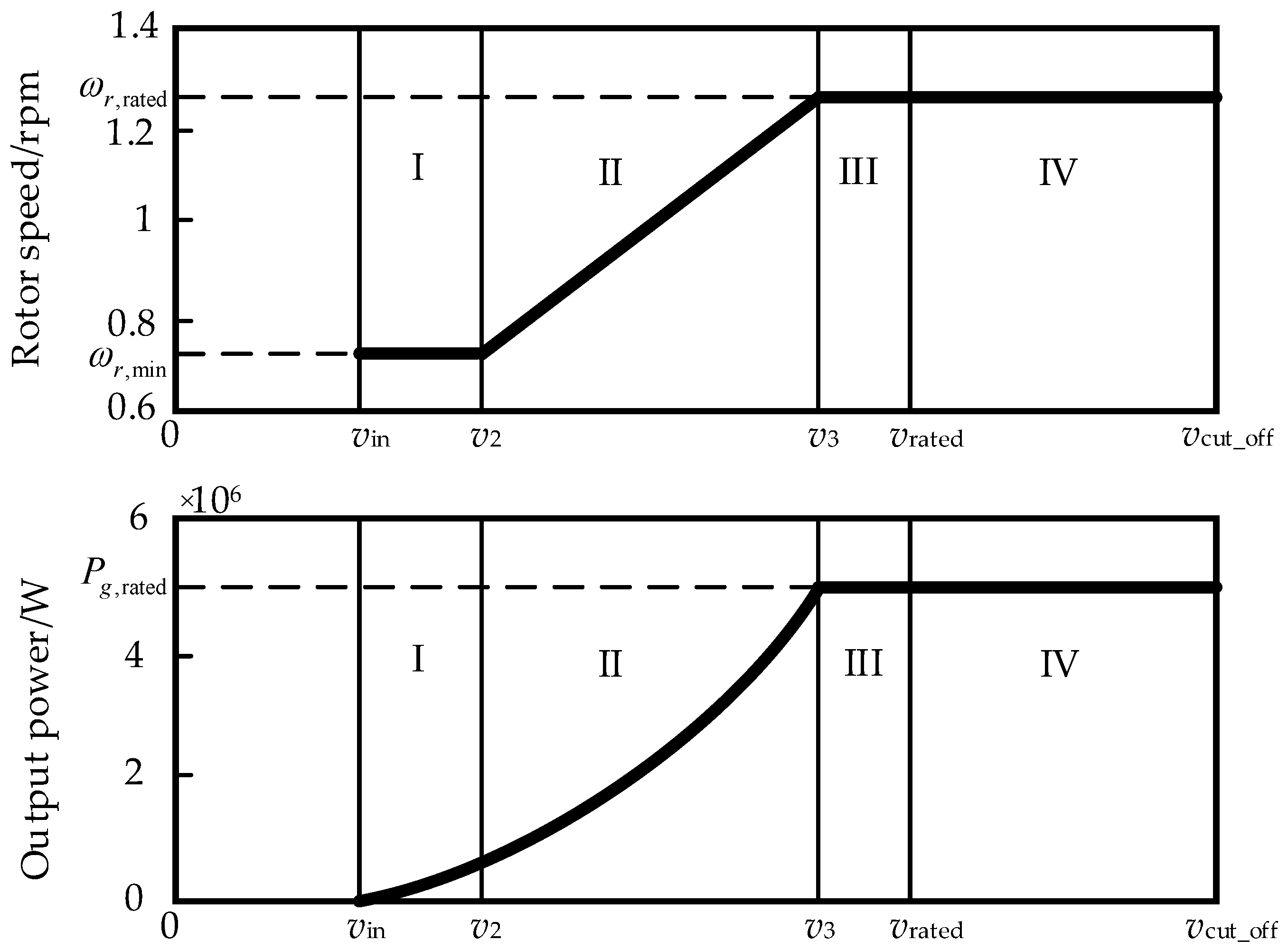
2. Wind Power Generation System Description

A WPGS is typically made up of three components: a turbine, a drive train, and a generator. Through a cascade of a low-speed shaft, gearbox, and high-speed shaft, the drive train converts aerodynamic torque captured from the wind energy to generator torque. Thus, for realizing an effective WPGS control, detailed modeling of wind speed and the WPGS is required, where the definitions of parameters for a 5 MW WPGS are listed in Table 1.

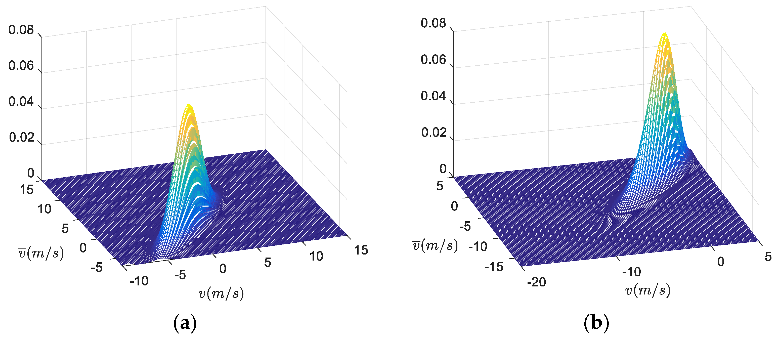
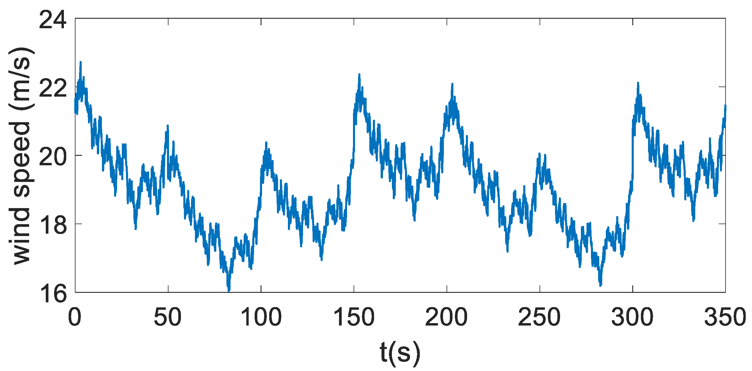
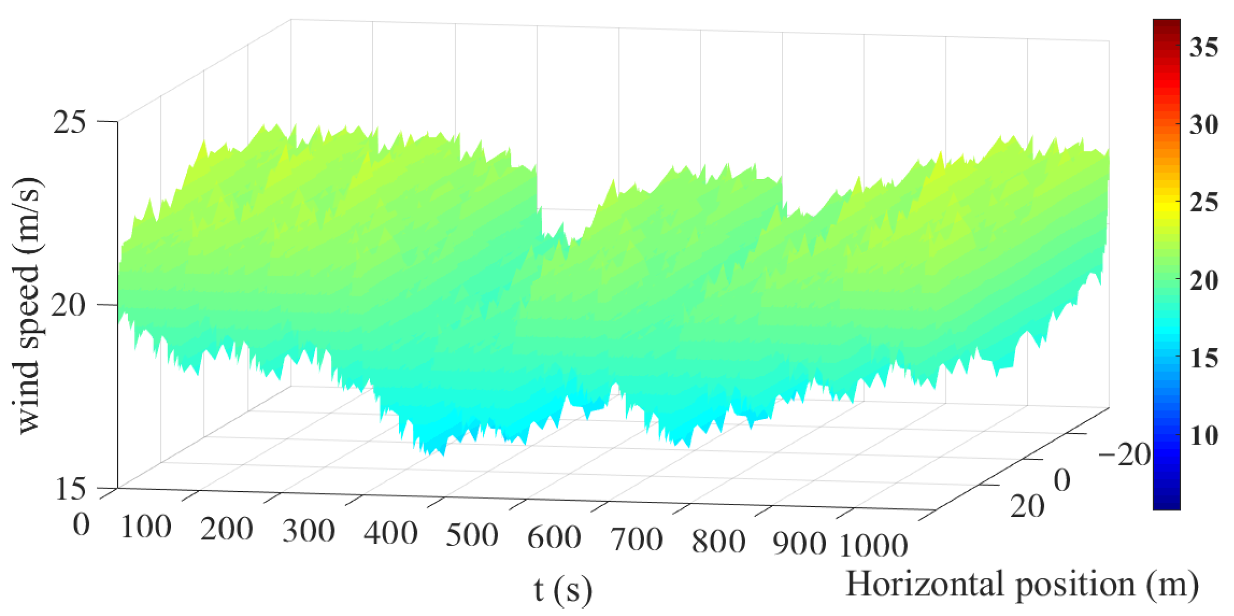
2.1. Wind Speed Model

In terms of wind energy, the most notable feature of wind resources is their variability which endures across a very wide range of scales, both in space and time. Practically, on a wide scale, spatial variability describes the reality that the planet has many diverse climatic zones, some of which are much windier than others. These regions are mostly influenced by latitude, which determines the quantity of insolation. Within any climatic zone, there is a considerable amount of diversity on a smaller scale, which is mostly dictated by physical geography (e.g., the proportion of land and sea, the size of landmasses, the presence of mountains or plains, the kind of flora, and topography). On the long timescale, although seasonal variations are predictable resulting from Earth revolution (such as tropical storms and cold-air outbreaks), they are not very predictable more than a few days ahead due to the changes in insolation caused by the tilt of the Earth’s axis of rotation. Meanwhile, there is also a diurnal component to wind speed turbulence induced by fluctuations in insolation caused by the Earth’s rotation. As a result, the non-stationary stochastic effective wind speed v applied to WPGS can be decomposed into the following two independent components [25]:
v = v m + v t .
In (1), mean wind speed v m represents the long-term slow-variable component, which obeys two-parameter Weibull distribution with scale parameter s 1 and shape parameter s 2 [26]:
v m ~ W e i b u l l ( v m ; s 1 , s 2 ) = s 2 s 1 ( v m s 1 ) s 2 1 exp ( ( v m s 1 ) s 2 ) .
Meanwhile, turbulent speed v t describes the rapid variable component, which is designed as a Gaussian distribution with standard deviation σ [25]:
v t ~ N ( 0 , σ 2 ) .
As v m and v t are independent according to (1), the wind disturbance v ¯ = v v have zero mean and the variance is
σ v = s 1 2 Γ ( 1 + 2 s 2 ) s 1 2 Γ 2 ( 1 + 1 s 2 ) + σ 2 ,
where v is the average wind speed value during the measurement interval T . Γ ( ) is the Gamma function widely used in probability theory.
According to (1)–(3), the probability density function (pdf) of wind speed disturbance v ¯ = v v can be obtained using convolution as:
f ( v ¯ ) = + g ( v , v ¯ ) d v = v + s 2 2 π σ s 1 ( v + v s 1 ) s 2 1 exp ( ( v + v s 1 ) s 2 ( v ¯ v ) 2 2 σ 2 ) d v .
The real wind speed disturbance must have an upper bound, i.e.,
| v ¯ ( t ) | γ 1 ,
where γ 1 is a nonnegative scalar.
Thus, with a small enough positive constant ε , it holds:
Pr ( | v ¯ ( t ) | γ 1 ) = 1 ε .
In real-time WPGS control, as the actual wind speed v is bounded by the cut-off value v cut _ off , the upper bound γ 1 must satisfy 0 < γ 1 < γ 0 with 0 < γ 0 < v cut _ off v .

2.2. WPGS Model

The original first-principal model, which can completely represent the dynamics of a WPGS, has been well established as [1,25,26,27,28]:
{ J r ω ˙ r = T r K s θ D s θ ˙ θ ˙ = ω r ω g N M J g ω ˙ g = T g + K s N M θ + D s N M θ ˙ P g = η g ω g T g ,
where the aerodynamic torque of the rotor T r is expressed as:
T r = 1 2 ρ π R 2 v 3 C p ( λ , β ) .
Here, the aerodynamic efficiency C p is related to the collective blade pitch angle β and the tip speed ratio λ = R ω r / v [29]:
C p ( λ , β ) = 0.5176 ( 116 λ s 0.4 β 5 ) exp ( 21 λ s ) + 0.006795 λ ,
where is determined using:
1 λ s = 1 λ + 0.08 β 0.035 β 3 + 1 .
If a set of state variables x = [ x 1 x 2 x 3 ] T = [ ω r θ ω g ] T and input variables u = [ u 1 u 2 ] T = [ β T g ] T are defined, the WPGS dynamics can be written in the following form under modeling Equations (8)–(10):
x ˙ = f ( x , u , v ) ,
where nonlinear function f ( x , u , v ) is a Lipschitz function.
The above WPGS is operated to track the steady targets for obtaining the optimal performance depending on the wind speed v . The entire operating region is divided into four regions under v in < v < v cut _ off , as shown in Figure 1 [30]. In WPGS control, the control objective in the low-speed region ( v in < v < v 3 ) is typically to track the maximum power point by regulating the generator torque T g with a fixed pitch angle β = 0 for obtaining maximum aerodynamic efficiency C p , max . In the high-speed region ( v 3 v < v cut _ off ), the basic control task is to adjust the blade pitch angle β in order to keep both the output power and the generator speed at their rated values to ensure the security of the equipment with a fixed value T g , rated [31,32]. Thus, the optimal steady-state target is obtained as follows [30]:
{ ω r = { ω r , min ,   if   v in v < v 2 λ o p t v / R ,   if   v 2 v < v rated ω r , rated ,   if   v rated v < v cut _ off θ = 0 ω g = N M ω r β = { 0 ,   if   v in v < v rated { β | P g , rated = 1 2 η g ρ π R 2 v 3 C p ( λ , β ) } ,   if   v rated v < v cut _ off T g = { ρ π R 2 v 3 C p ( ω r , min R / v , 0 ) / ( 2 ω r , min N M ) ,   if   v in v < v 2 { T g | 0.5 ρ π R 2 v 3 C p , max = N M λ opt v T g / R } ,   if   v 2 v < v 3 ρ π R 2 v 3 C p ( ω r , rated R / v , 0 ) / ( 2 ω r , rated N M ) ,   if   v 3 v < v rated T g , rated ,   if   v rated v < v cut _ off .

3. Model Predictive Control Strategies
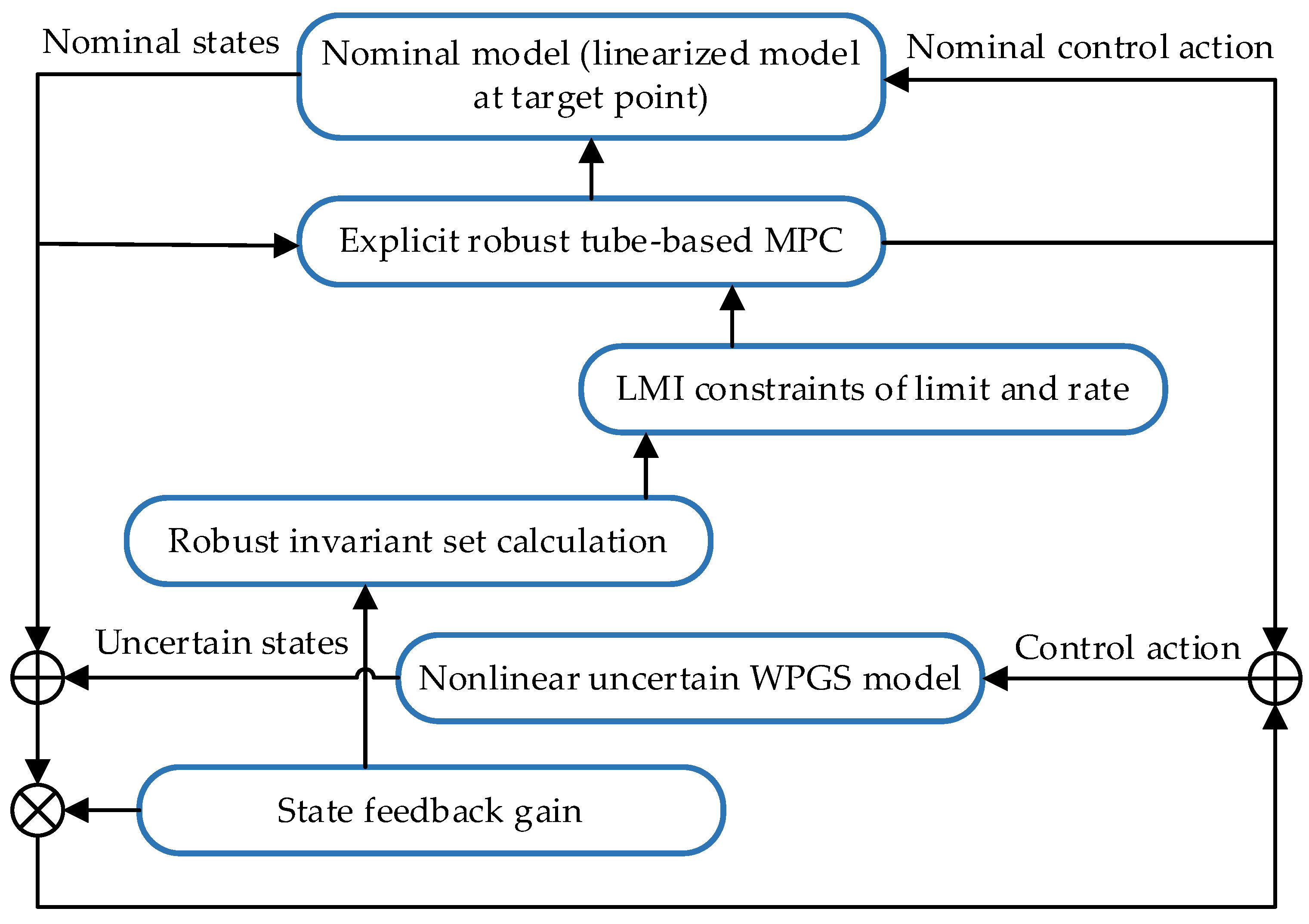
3.1. Robust MPC

The wind dependent reference trajectories are tracked by the robust MPC for WPGS. As previously indicated, various control goals exist for different operating modes. The robust MPC achieves this through modifying the reference. In terms of WPGS state constraints, both hard and soft constraints are incorporated in the optimization problem. At a sample time t k , the MPC optimization problem for the WPGS, for both partial load region and full load region, is described as follows:
min u ( τ ) S ( Δ t ) t k t k + N J ( x ˜ ( τ ) , u ( τ ) ) d τ ,
subject to (s.t.),
x ˜ ˙ = f ( x ˜ ( τ ) , u ( τ ) , v ( τ ) ) ,
x ˜ ( t k ) = x ( t k ) ,
0 P g ( t ) P g , rated + ε P ,
β min β ( t ) β max ,
β ˙ min β ˙ ( t ) β ˙ max ,
0 T g ( t ) T g , rated ,
T ˙ g , min T ˙ g ( t ) T ˙ g , max ,
where S ( Δ t ) denotes the family of continuous piece-wise functions with sampling time Δ t . N represents the predictive horizon. x ˜ ( τ ) represents the predicted state trajectory of the WPGS. Equation (14) is the nonlinear state-space model of the WPGS base on Equation (11). x ( t k ) in Equation (15) is the initial condition at time t k . Equation (16) is the output power constraint due to the limitations of mechanical components for ensuring system security, which is the precondition of the WPGS operation through restraining the damage caused by the extreme high loads. ε P = 0.1 P g , rated is a looseness parameter. Equations (17)–(20) are the constraints of pitch angle and the generator torque. The objective function is chosen as [27,30]:
J ( x ( t ) , u ( t ) ) = r 1 β ˙ ( t ) 2 + r 2 T ˙ g ( t ) 2 + r 3 ( P g ( t ) P g ) 2 .
The first and second term of objective function (21) reflect the structural fatigue of the system while the last term accounts for wind power capture. For the tuning parameters, large values of r 3 in relative to r i (i = 1,2) reflect the intention to drive the output power quickly to the target value at the expense of significant control action. Penalizing the control action through larger values of r i (i = 1,2) relative to r 3 can slow down the control action rate at which the output power approaches the target value.
As the predictive output power depends on the future control move, an explicit linear relation between u and x is not available from the nonlinear wind turbine system (11). To facilitate solving the nonlinear optimization problem (13), it is necessary to linearize the model (11) around the operating point to facilitate the online optimization. Therefore, on the premise of satisfying constraints (16)–(20), the optimization problem of robust MPC is constructed by utilizing the boundary condition, expressed as:
min u ( τ ) S ( Δ t ) max w W t k t k + N J ( x ˜ ( τ ) , u ( τ ) ) d τ ,
s.t.,
x ¯ ˙ ( τ ) = A ¯ l x ¯ ( τ ) + B ¯ l u ¯ ( τ ) + w ( τ ) ,
x ˜ ( t k ) = x ( t k ) ,
x ˜ ( τ ) = x ¯ ( t k ) + x ,
u ( τ ) = u ¯ ( τ ) + β ,
x ¯ ( t k ) = x ( t k ) x ,
where Equation (23) denotes the prediction model. External additive bounded disturbance w includes the linearized higher-order term and stochastic uncertainty caused by wind speed disturbance, which lies in the set W derived by Lipschitz condition [33]. The coefficient matrix A ¯ l and B ¯ l are obtained by linearizing the Function (11) around the optimal reference point ( x , u ) , i.e.,
A ¯ l = f ( x , u , v ) x | ( x , u ) ,   B ¯ l = f ( x , u , v ) u | ( x , u ) .
However, there exists a huge calculation burden to search for the optimal solution by enumerating all the vertices of W in the prediction horizon. Thus, an efficient tube method is incorporated to solve the min–max optimization problem (22) to reduce the calculation burden [20]. The controller is evaluated at discrete time instants t k = t 0 + k Δ t , k = 0 , 1 , , with the initial time t 0 and the sampling time Δ t . If the optimal solution to the optimization problem (22) is denoted as u RMPC ( t | t k ) , only the first step value of u RMPC ( t | t k ) is applied to the WPGS, i.e.,
u ( t ) = u RMPC ( t | t k ) , t [ t k , t k + 1 ) .
The robust MPC optimization issue is re-evaluated at the next sample time. Overall, the robust MPC algorithm for WPGS is designed by utilizing the explicit tube-based robust MPC, consisting of offline and online calculations (given below). Figure 2 shows how the control signal is formed.
Offline calculations:
  • The linearized model (23) is calculated at the target point as in (23) under the measurement wind speed.
  • The additive uncertainty w is calculated using the Lipschitz condition.
  • The robust invariant set is calculated utilizing the general robust tube method based on a predefined state feedback gain and boundary parameter γ 1 in (7).
  • The constraints (16)–(20) are transformed into the LMI forms on the basis of the robust invariant set.
Online calculations:
  • The optimal control sequence is calculated by solving an explicit tube-based robust MPC under the current state.
  • Only the first two elements of the optimal control sequence are applied to the nominal model.
  • The state error between the nominal model and the nonlinear uncertain system is calculated.
  • The total control signal is calculated and then applied to the WPGS.
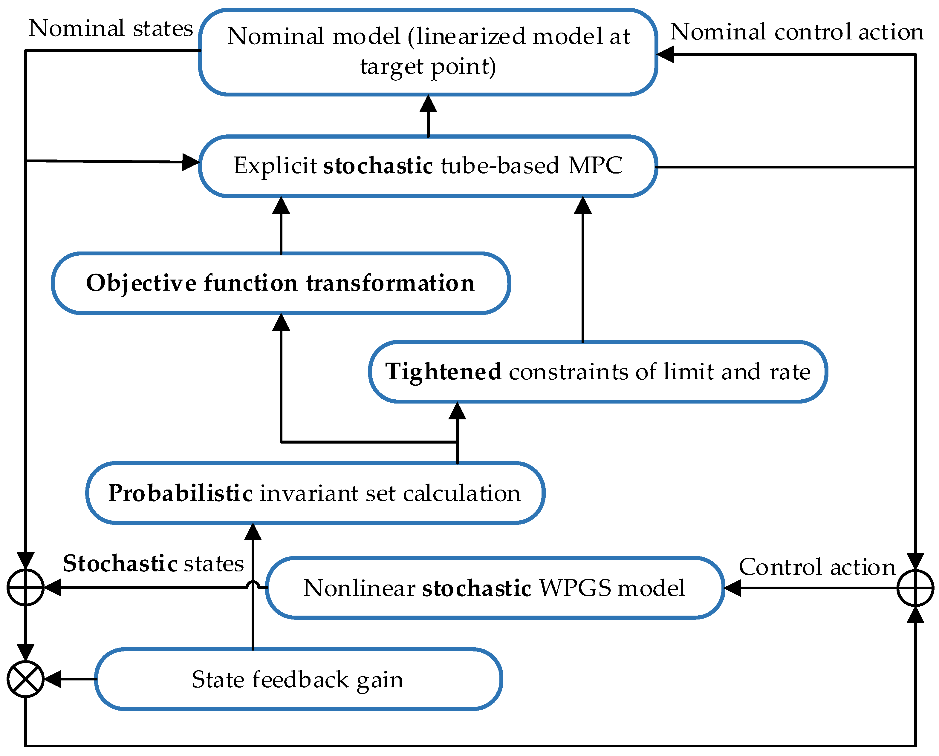
3.2. Stochastic MPC

Considering that the main control objective of WPGS in high wind speed region is to maintain the output power at the rated value, the output power may fluctuate around the rated value (i.e., 5 MW) due to the stochastic wind speed disturbance. However, if the output power frequently exceeds the rated value, it can cause damage to the WPGS and lead to high maintenance cost. To reduce this damage, the probabilistic limitation on the output power based on constraint (16) has been incorporated into the WPGS stochastic control problem.
Pr { 0 < P g ( t ) P g , rated } > p ,
where confidence level p ( 0 , 1 ) is a probability given in advance for trading off the security and the optimality.
In summary, owing to the stochasticity of WPGS, a general stochastic MPC optimization problem on this WPGS subject to Equations (14)–(20) and (30) can be denoted as:
min u ( τ ) S ( Δ t ) E ( t k t k + N J ( x ˜ ( τ ) , u ( τ ) ) d τ ) ,
where Equation (31) represents the expectation of objective function (21) should be optimized based on the distribution of wind speed (5) at each time instant [24].
Notice that the stochastic optimization problem (31)) with the probabilistic constraint (30) cannot be solved by deterministic optimization routines. This stochastic optimization problem can be solved efficiently by using the well-established tube-based stochastic MPC algorithm, while the feasibility of the controller can be guaranteed [34,35]. Figure 3 shows the construction of stochastic MPC for WPGS. In this method, the probabilistic invariant set can be calculated based on the wind speed stochastic disturbance probability information after a proper linearization process. Subsequently, the stochastic optimal problem can be transformed into a deterministic one by utilizing the probabilistic invariant set. The following optimal solution is then applied to the WPGS:
u ( t ) = u SMPC ( t | t k ) , t [ t k , t k + 1 ) .
The overall process of the stochastic tube-based MPC is similar to the robust tube-based MPC. It is worth noting that there exist some changes in the details of the controller design:
  • The probabilistic invariant set is calculated by utilizing the boundary parameter γ 2 where Pr ( | v ¯ ( t ) | γ 2 ) = p .
  • The expectation of objective function (21) is transformed into a deterministic one for facilitating the online solving of the stochastic optimization problem (31)).

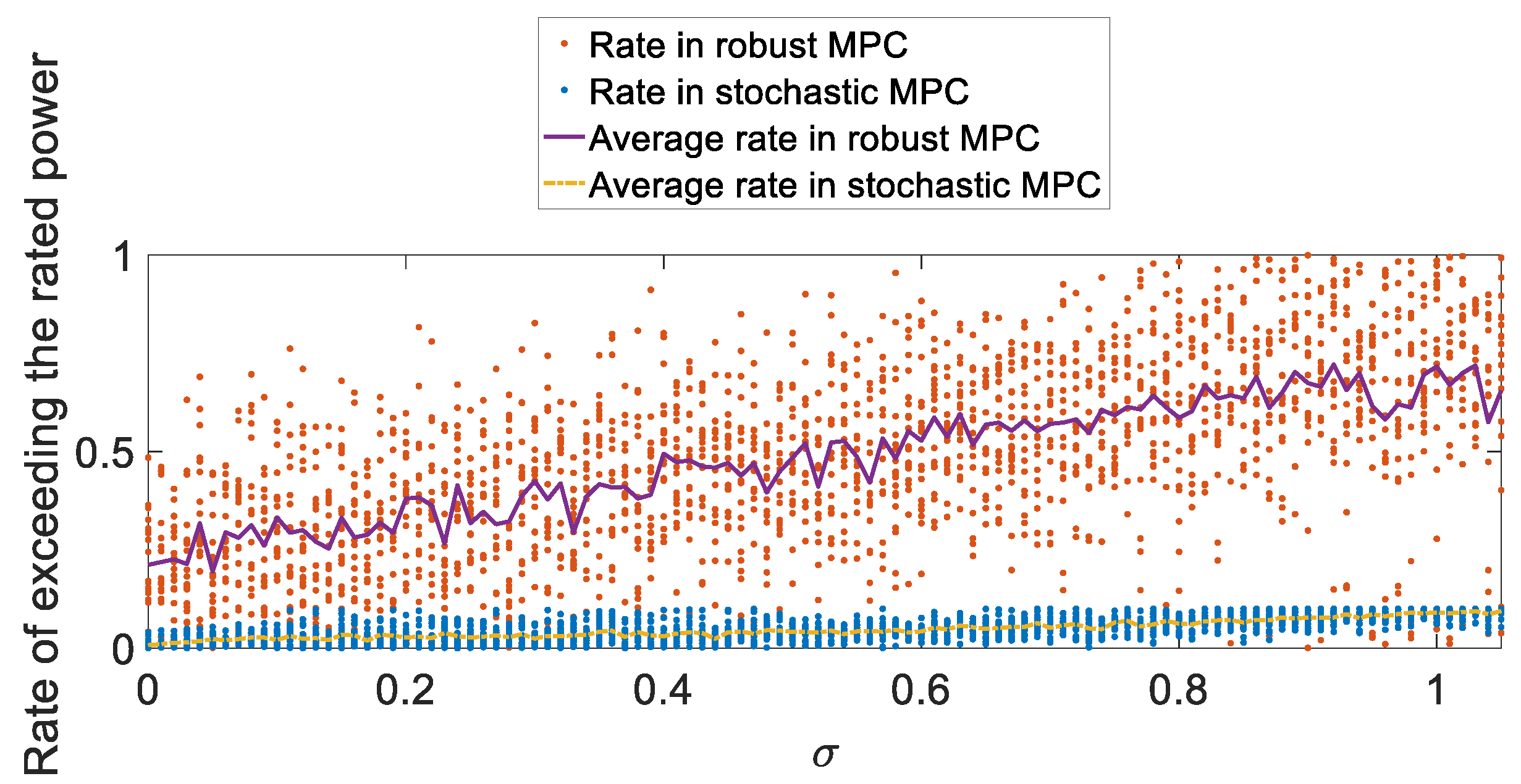
4. Simulation Results

In this section, simulations are carried out to contrast the robust MPC versus the stochastic MPC in terms of optimal performance, such as the generated rated output power P g , the drivetrain shaft transient load torsion θ , and the probabilistic constraint violation rate. Different wind speeds containing slight and severe high turbulent wind speed are generated by model (1) and TurbSim. Besides the WPGS model (8), the practicality of the robust MPC and the stochastic MPC strategy is also validated on an aeroelastic simulator for WPGS, named FAST (fatigue, aerodynamics, structures, and turbulence).

4.1. Simulation Settings

The values of parameters for the 5 MW WPGS from the National Renewable Energy Laboratory (NREL) are listed in Table 2 [36]. We set the control horizon n c = 10 , and the sampling interval T s = 0.05 s . In the objective function (21), the weight parameters are selected as r 1 = 7 , r 2 = 1 × 10 - 8 , and r 3 = 1 × 10 - 12 [9,27].
According to the stochastic wind speed model (Equations (1)–(3)), the Weibull distribution with the scale parameter s 1 and the shape parameter s 2 are adopted to depict the low-frequency component v m , while the Gaussian distribution with the variance σ is utilized to depict the high-frequency component v t . These parameters can be obtained through maximum likelihood estimation, Bayesian network, or other proper statistical methods based on the wind speed data monitored by the supervisory control and data acquisition (SCADA) system, which collects the condition parameters containing wind speed and wind direction with a one-second interval from the wind farm located on China’s southeast coast. Thus, the distribution of function in low and high wind speed region in this simulation part is clearly shown in Figure 4, according to measurement wind speed 8 m/s and 20 m/s in different regions, respectively.
The wind speed variations are somewhat more stochastic and less predictable on shorter timescales than the longer timescales. The parameter σ in (3) represents the standard deviation of the Gaussian distribution, which reveals the magnitude variation of the turbulent wind speed v t . When σ surpasses a threshold value, the WPGS will be cut-off.
In the simulation validation, it should be ensured that the generated wind speed, exceeding the cut-off wind speed v cut _ off = 25 m/s, is a small probability event. In probability theory, events that occur with a probability of 0.01 or less are usually defined as small probability events, i.e., events that are almost impossible to occur. Thus, the generated wind speed is required to fall in the interval [ v , v cut _ off v ] with 99% confidence:
0.99 = v v c u t _ o f f v f ( v ¯ ) d v ¯ = v v c u t _ o f f v v + s 2 2 π σ s 1 ( v + v s 1 ) s 2 1 exp ( ( v + v s 1 ) s 2 0.5 ( v ¯ v ) 2 σ 2 ) d v d v ¯
Thus, the limit of σ can be obtained when parameters s 1 , s 2 , and v are determined.

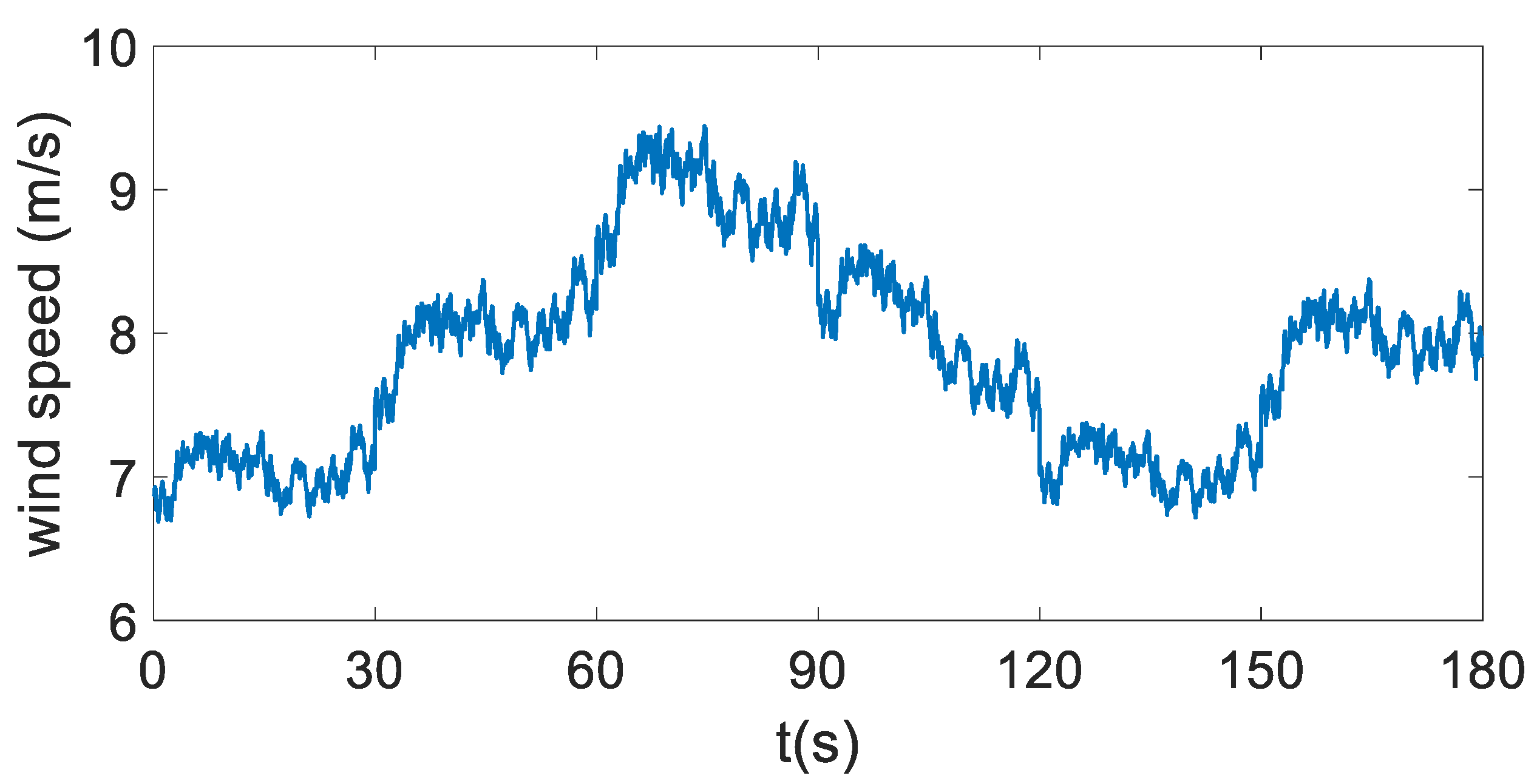
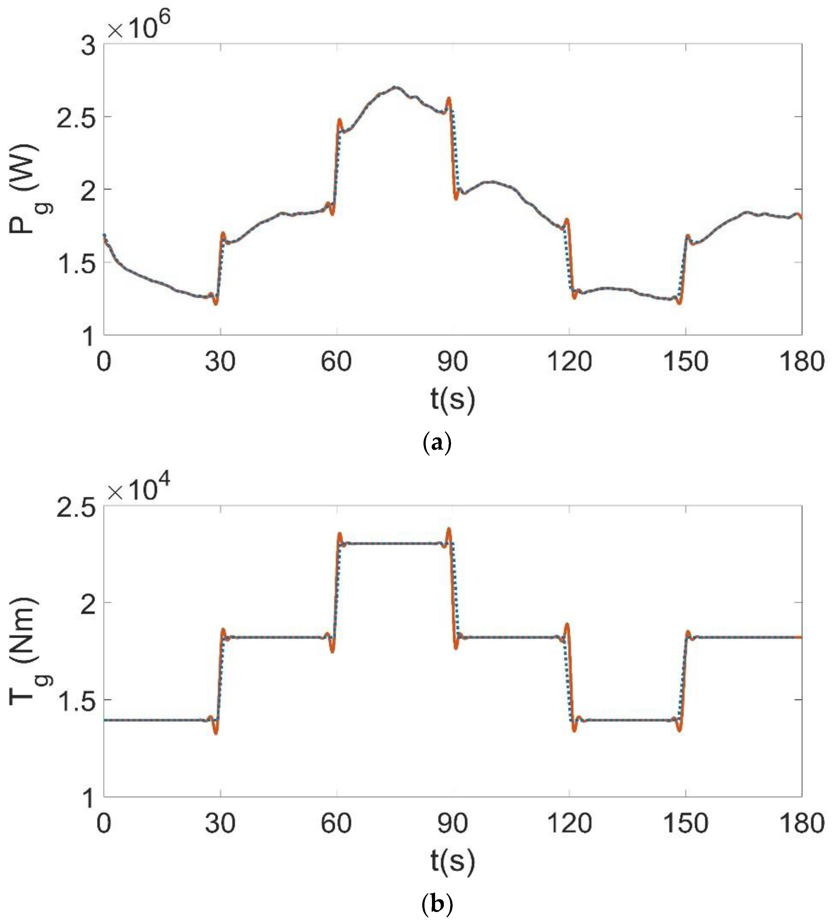
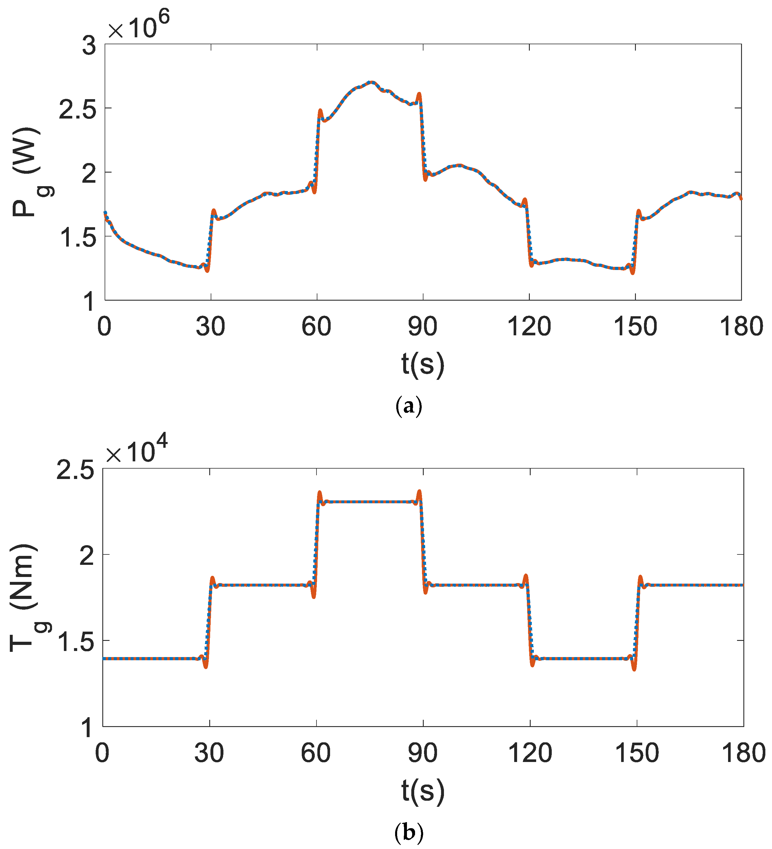
4.2. Low Wind Speed Region

The Weibull distribution with parameters s 1 = 9 and s 2 = 4 is chosen to characterize the stochastic properties of the mean wind speed at low wind speed region, i.e., a sequence of mean wind speeds { v m , 0 , v m , 1 , , v m , 5 } = { 7 , 8 , 9 , 8 , 7 , 8 } varying every 30 s over a 180 s period is selected. For analyzing the effect of turbulent wind speed intensity on the controllers, the following scenarios are designed to compare the control performance of the two controllers for small and large turbulent wind speeds, respectively. Throughout the simulation, the steady-state point is set to be the equilibrium point at v m = 8 m/s, where the initial point x 0 is a point within a small neighborhood of the steady-state point, i.e., [ 0 . 914 0 . 0002 90 . 505 ] T .

4.2.1. Slight Turbulence Condition

The turbulence intensity in the TurbSim input file is set as 1.5%, corresponding to the standard deviation σ = 0.1 in Gaussian distribution for simulating the slight turbulence. The generated turbulent wind speed is appended to the sequence of mean wind speeds to simulate more realistic wind speeds, as shown in Figure 5. The boundary parameter γ 1 = 3.063 is obtained according to Equation (6).
Figure 6 shows that there is no significant difference between robust MPC and stochastic MPC for WPGS from the essentially same output power tracking and generator torque response. This is due to the fact that when the WPGS operates in the low wind speed region, the output power does not exceed the rated power and therefore the probability constraints in the stochastic MPC strategy are not violated, resulting in essentially the same effect as in robust MPC.
It can also be seen from Figure 6 that the robust MPC has a relatively larger fluctuation at the transient moments. As the robust MPC strategy considers the boundary of the wind speed rather than the stochastic information, it can incur less optimality and high conservativeness in controlling WPGS. When the system’s stochastic uncertainties have been adequately characterized by probabilistic descriptions, it is incorporated into a stochastic optimal control problem. The stochastic MPC has a relatively better performance at the transient moments than the robust MPC.

4.2.2. Severe Turbulence Wind Speed Condition

The turbulence intensity in the TurbSim input file is set as 15% corresponding to the standard deviation σ = 1 in Gaussian distribution for simulating the severe turbulence. The generated turbulent wind speed is appended to the sequence of mean wind speeds to simulate more realistic wind speeds, as shown in Figure 7. The boundary parameter γ 1 = 3.572 is obtained as according to Equation (6).
Figure 8 depicts the response of output power and generator torque under the wind speed condition in Figure 7. From this figure, the control effectiveness of the WPGS under robust MPC and stochastic MPC is essentially indistinguishable from the case with slight turbulence. This is because the stochastic MPC control law needs to be solved offline using the boundary information γ 1 of wind speed disturbance for calculating the probabilistic invariant set, and subsequently obtaining the optimal control law for the linearized stochastic dynamic model within this probabilistic invariant set. For guaranteeing that the output power does not exceed the rated value with probability 0.9, the stochastic distribution of wind speed disturbances is utilized to calculate this boundary information. As the probability constraint (30) on the output power Pg is usually easily guaranteed in the low wind speed region, it is clear from the stochastic MPC scheme that changes of variance σ characterizing the magnitude of the turbulence do not cause a significant influence in the stochastic MPC calculation compared to the slight turbulence case, i.e., the probability constraint (30) of output power has not been excited.

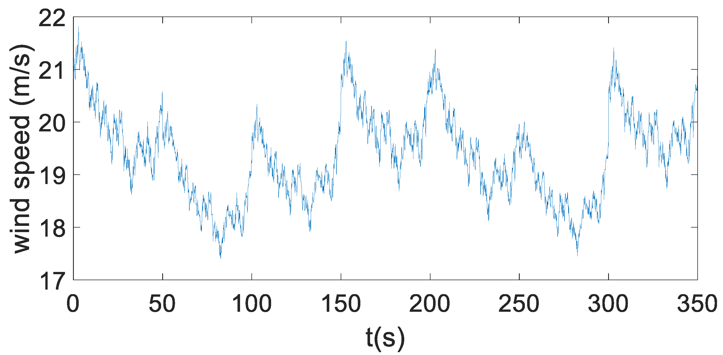
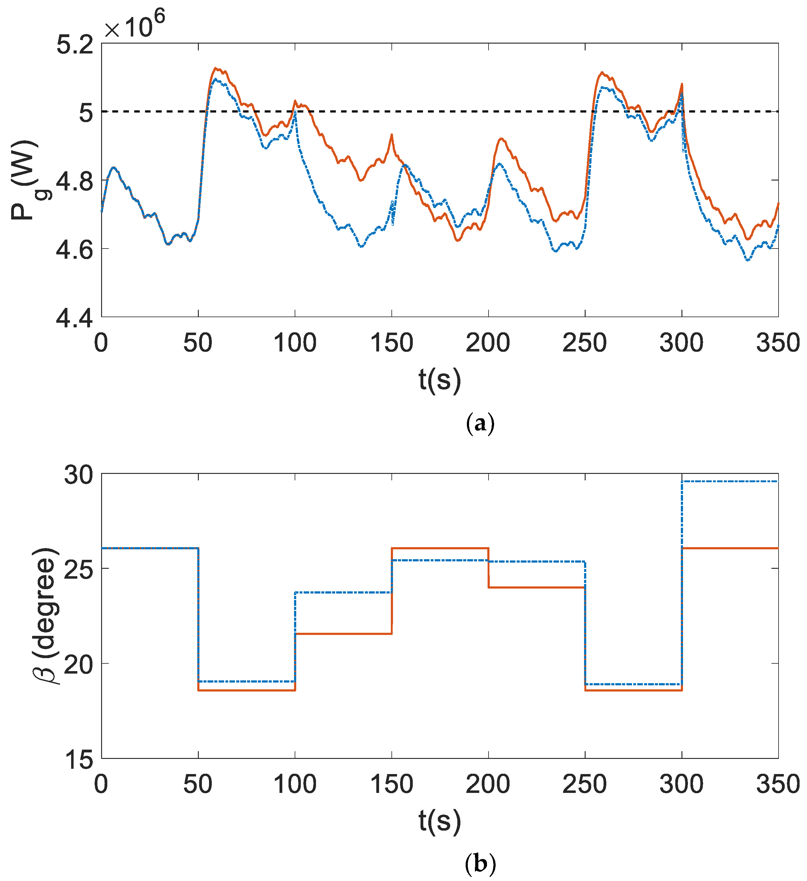
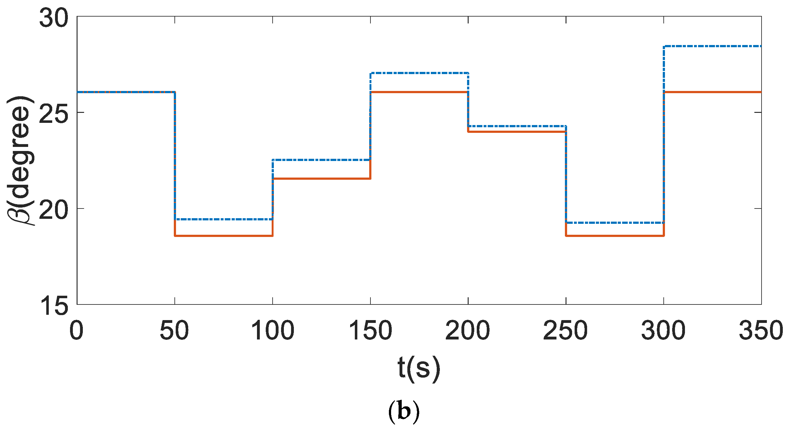
4.3. High Wind Speed Region

The Weibull distribution with parameters s 1 = 21 and s 2 = 11 is chosen to characterize the stochastic properties of the mean wind speed at high wind speed region, i.e., a sequence of mean wind speeds { v m , 0 , v m , 1 , , v m , 7 } = { 20 , 17 , 18 , 20 , 19 , 17 , 20 } varying every 30 s over a 180 s period is selected.
In order to analyze in detail the effect of turbulent wind speed intensity on the effectiveness of the controller, the following scenarios were designed to compare the control performance of the two controllers for small and large turbulent wind speeds, respectively. Throughout the simulation, the steady-state point is set to be the equilibrium point at v m = 20 m/s, wherein the initial point x 0 is [ 0.914 0.0002 90.505 ] T .

4.3.1. Slight Turbulence Condition

The turbulence intensity in the TurbSim input file is set as 15%, corresponding to the Gaussian distribution for simulating the severe turbulence in this scenario.
The generated turbulent wind speed with standard deviation σ = 1 by TurbSim is appended to the sequence of mean wind speeds to simulate more realistic wind speeds, as shown in Figure 9. The boundary parameter γ 1 = 4.235 is obtained as according to Equation (6).
Figure 10 depicts the system response under both the robust MPC and the stochastic MPC. It is clearly shown that both controllers manage to capture the rated wind energy. The stochastic MPC ensure the security of WPGS by incorporating probabilistic constraint (30) to reduce the rate of exceeding the rated power Pg,rated, while keeping a similar average value of output power Pg. Furthermore, the stochastic MPC reaches a higher optimality. Table 3 lists these comparison results.

4.3.2. Severe Turbulence Wind Speed Condition

The turbulence intensity in the TurbSim input file is set as 15% corresponding to the standard deviation σ = 1 of Gaussian distribution. Under the same mean wind speed sequence as Section 4.3.1, the resulting wind speed is shown in Figure 11. Similarly, the corresponding boundary parameter can be obtained as γ 1 = 4.703 .
The system response under this wind speed condition is shown in Figure 12. Compared with a slight turbulence condition (Figure 10), the probability of satisfying the constraint 0 < P g ( t ) P g , rated is also kept in 0.1, signifying the restricting of the rate of exceeding the rated output power Pg,rated. Table 4 lists the comparison results between the two controllers. The rate of exceeding the rated power Pg,rated in robust MPC is 1.863 times larger than that in stochastic MPC. Compared with the slight turbulent condition, the increasing rate of exceeding the rated power Pg,rated in robust MPC and stochastic MPC are 3.31% and 0.61%, respectively.
According to Equation (33), the limit of σ is obtained as 1.05 in the high wind speed region. Therefore, simulations are then performed under 106 different σ ( σ = 0.01 i , i = 0 , 1 , , 105 ) to test the influence of the parameter σ on the rate of exceeding the rated power P g , rated . The two sets of the polylines and scattered points in Figure 13 show this rate in robust MPC and stochastic MPC for 20 realizations of the stochastic wind speed disturbance under each σ . From Figure 13, the average rate in both controllers grows with the increasing σ . However, the increase in robust MPC is much faster, while the rate in stochastic MPC never exceed 10% due to the incorporation of the probabilistic constraint (30).

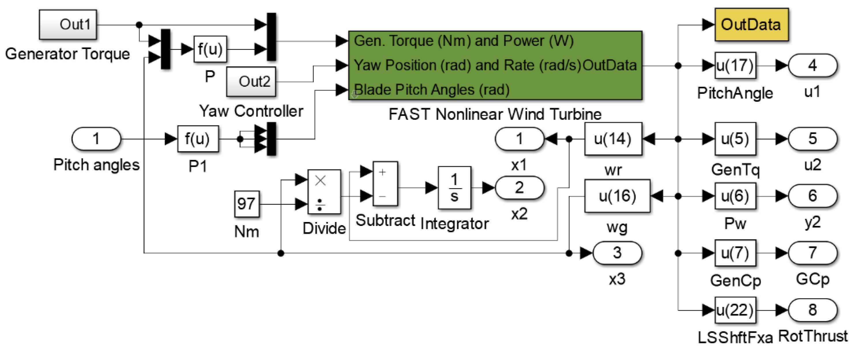
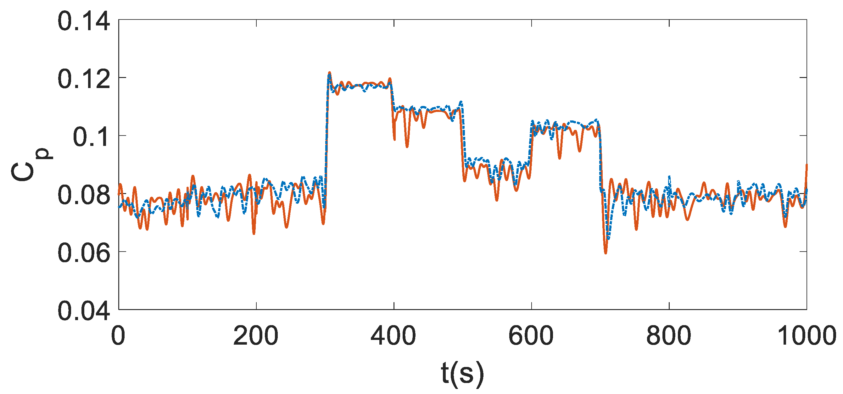
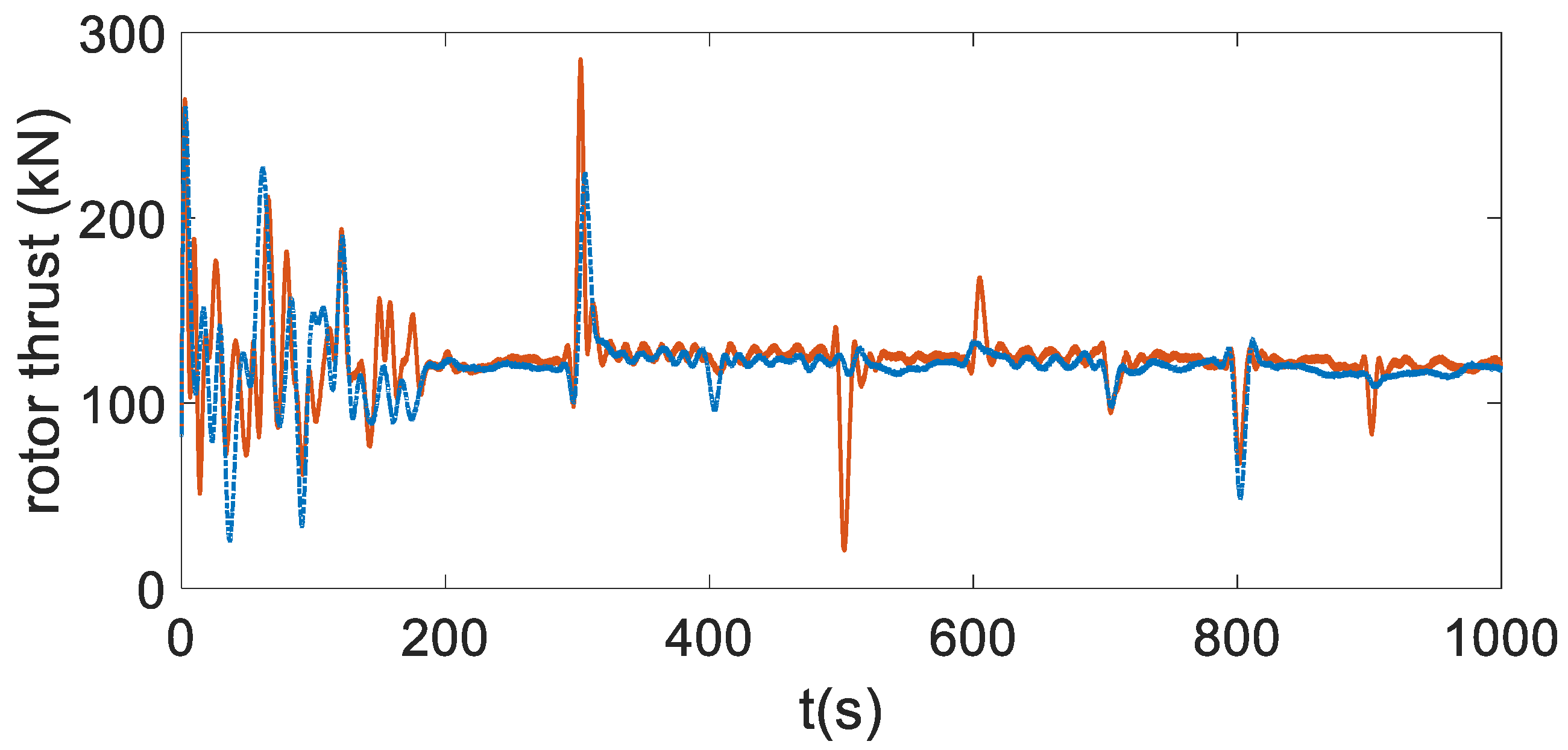
4.4. Validation Using FAST Simulator

To further compare the practicality of the robust MPC and stochastic MPC, simulations are then performed in a high wind speed region with severe turbulence using the FAST simulator, which uses the blade element momentum theory to conduct more detailed modeling and simulation of wind turbine aerodynamics. In this experiment, the 24 degrees of freedom (DOFs) model is enabled in the FAST simulator. The FAST program is written into an S-Function so that it can be incorporated into a MATLAB Simulink scheme, shown in Figure 14.
Under the mean wind speed sequence { v m , 0 , v m , 1 , , v m , 7 } = { 20.2 , 20.1 , 19.9 , 17.9 , 18.1 , 19.6 ,   18.3 , 19.2 , 19.8 , 20.4 } , the spatial wind speed generated by TurbSim is shown in Figure 15.
The power coefficient C p is defined as the ratio of the mechanical power extracted by the turbine to the power in the air stream. It is usually given as a function relating to two parameters: the tip–speed ratio λ and the pitch angle β . The power coefficient C p (shown in Equation (10)) is obtained c based on a large number of monitoring data [29,37]. This C p expression is therefore adopted in controller design, and then used in the simulation for comparing the effectiveness of the robust MPC and stochastic MPC. In existing research work, the FAST module has been well utilized to simulate 5 MW wind turbine experimental verification [37,38,39]. As the power coefficient C p in FAST is obtained from a look-up table, there will inevitably exist deviation between the C p in model (10) and C p in FAST. From Figure 16, the C p in Equation (10) can fit the C p in FAST well when under the same wind speed condition shown in Figure 15. It is therefore accurate enough to be used in controller design.
The system responses in robust MPC and stochastic MPC are depicted in Figure 17. Table 5 lists the comparison results between the two controllers. From Figure 17 and Table 5, the rate of exceeding the rated power Pg,rated in stochastic MPC can be maintained within 10%, which is much less than that in robust MPC. The proposed stochastic MPC strategy decreases the optimal index (21) while keeping similar average value of output power with that of the robust MPC strategy. The stochastic MPC realizes a lower rate of exceeding the rated power, even though the average output power in stochastic MPC is a little bit lower than that in robust MPC. This indicates that the system security has been guaranteed due to the incorporation of probabilistic constraint (30).
In WPGS operation, the drive torque is transferred from the rotor hub to the gearbox by low-speed shaft. Meanwhile, the rotor load should be transferred to the nacelle structure without experience deflections which would compromise the proper operation of the gears and subject the wind turbine to a severe fatigue loading regime. Fatigue analysis is complicated in that it requires the superposition of stress histories resulting from simultaneous time histories of up to six rotor load components (e.g., rotor thrust, yaw moment, tilt moment, and so on) derived from simulations at different determined wind speeds using finite-element analysis [1]. Thus, it is crucial to appropriately choose a load component for quantitatively reflecting the wear and tear of the WPGS in fatigue analysis. Considering the full-order FAST module is performed in this experiment, the main component of the rotor load–rotor thrust in FAST is used to predict the fatigue load of wind turbines and the mechanical life of the unit. The comparison of rotor thrust under different controllers is depicted in Figure 18.
From Figure 18, the stochastic MPC reduces the rotor thrust compared with the robust MPC by incorporating the stochastic characteristics of wind speed and the probabilistic constraint of output power in the controller design, which further reduces the wear and tear to prolong the turbine lifetime.

5. Conclusions

This paper focuses on the comparison of a robust MPC and stochastic MPC for a typical WPGS with wind speed disturbance. From the simulation results, the robust MPC and the stochastic MPC may provide similar performance when the WPGS is operated in low wind speed regions considering turbulent wind speed with slight and severe intensity. When the WPGS is operated in the high wind speed regions, the performance of the stochastic MPC scheme tends to be highly sensitive to the stochasticity of the measured wind speed. The relationship between the robust MPC and the stochastic MPC is also explored, and the results were useful in explaining the two MPCs’ differing behavior. In summary, both robust MPC and stochastic MPC are promising optimal control strategies for WPGSs with wind speed disturbance. Stochastic has the potential to significantly reduce the damage risk caused by frequent violation of output power exceeding the rated value while keeping similar average output power under robust MPC. Future research topics include the development of distributed MPCs that are robust to the wind farm noise and stochastics wind speed disturbance.

Author Contributions

Conceptualization, X.L. and L.F.; Methodology, X.L. and L.F.; Project administration, X.L.; Software, L.F.; Supervision, X.L. and X.K.; Validation, L.F. and X.K.; Writing—original draft, L.F.; Writing—review and editing, X.L. and X.K. All authors have read and agreed to the published version of the manuscript.

Funding

This research was funded by the National Key Research and Development Program of China under Grant 2021YFE0190900; the National Natural Science Foundation of China under Grant 62073136, Grant 61833011; and the Central University Basic Research Fund of China under Grant 2020MS016.

Institutional Review Board Statement

Not applicable.

Informed Consent Statement

Not applicable.

Data Availability Statement

Not applicable.

Conflicts of Interest

The authors declare no conflict of interest.

References

  1. Burton, T.; Sharpe, D.; Jenkins, N.; Bossanyi, E. Wind Energy Handbook; John Wiley & Sons Ltd: Chichester, UK, 2001; pp. 293–297. [Google Scholar]
  2. International Energy Agency, Renewables 2021 Analysis and Forecasts to 2026. 2021. Available online: https://iea.blob.core.windows.net/assets/5ae32253-7409-4f9a-a91d-1493ffb9777a/Renewables2021-Analysisandforecastto2026.pdf (accessed on 30 April 2022).
  3. Ren, Y.; Li, L.; Brindley, J.; Jiang, L. Nonlinear PI control for variable pitch wind turbine. Control Eng. Pract. 2016, 50, 84–94. [Google Scholar] [CrossRef] [Green Version]
  4. Calabrese, D.; Tricarico, G.; Brescia, E.; Cascella, G.L.; Monopoli, V.G.; Cupertino, F. Variable structure control of a small ducted wind turbine in the whole wind speed range using a Luenberger observer. Energies 2020, 13, 4647. [Google Scholar] [CrossRef]
  5. Moradi, H.; Vossoughi, G. Robust control of the variable speed wind turbines in the presence of uncertainties: A comparison between H and PID controllers. Energy 2015, 90, 1508–1521. [Google Scholar] [CrossRef]
  6. Wei, C.; Zhang, Z.; Qiao, W.; Qu, L. An adaptive network based reinforcement learning method for MPPT control of PMSG wind energy conversion systems. IEEE Trans. Power Electron. 2016, 31, 7837–7848. [Google Scholar] [CrossRef]
  7. Saenz-Aguirre, A.; Zulueta, E.; Fernandez-Gamiz, U.; Lozano, J.; Lopez-Guede, J.M. Artificial neural network based reinforcement learning for wind turbine yaw control. Energies 2019, 12, 436. [Google Scholar] [CrossRef] [Green Version]
  8. Sun, B.H.; Tang, Y.; Ye, L.; Chen, C.Y.; Zhang, C.H.; Zhong, W.Z. A frequency control strategy considering large scale wind power cluster integration based on distributed model predictive control. Energies 2018, 11, 1600. [Google Scholar] [CrossRef] [Green Version]
  9. Kong, X.B.; Ma, L.L.; Liu, X.J.; Abdelbaky, M.A.; Wu, Q. Wind turbine control using nonlinear economic model predictive control over all operating regions. Energies 2020, 13, 184. [Google Scholar] [CrossRef] [Green Version]
  10. Soliman, M.; Malik, O.P.; Westwick, D.T. Multiple model multiple-input multiple-output predictive control for variable speed variable pitch wind energy conversion systems. IET Renew. Power Gen. 2011, 5, 124–136. [Google Scholar] [CrossRef]
  11. Abdelbaky, M.A.; Liu, X.J.; Jiang, D. Design and implementation of partial offline fuzzy model-predictive pitch controller for large-scale wind-turbines. Renew. Energy 2020, 45, 981–996. [Google Scholar] [CrossRef]
  12. Koerber, A.; King, R. Combined feedback–feedforward control of wind turbines using state-constrained model predictive control. IEEE Trans. Control Syst. Technol. 2013, 21, 1117–1128. [Google Scholar] [CrossRef]
  13. Kim, D.Y.; Kim, Y.H.; Kim, B.S. Changes in wind turbine power characteristics and annual energy production due to atmospheric stability, turbulence intensity, and wind shear. Energy 2021, 214, 119051. [Google Scholar] [CrossRef]
  14. Ouari, K.; Rekioua, T.; Ouhrouche, M. Real time simulation of nonlinear generalized predictive control for wind energy conversion system with nonlinear observer. ISA Trans. 2014, 53, 76–84. [Google Scholar] [CrossRef] [PubMed]
  15. Zhao, H.; Wu, Q.; Guo, Q.; Sun, H.; Xue, Y. Distributed model predictive control of a wind farm for optimal active power control part I: Clustering-based wind turbine model linearization. IEEE Trans. Sustain. Energy 2015, 6, 831–839. [Google Scholar] [CrossRef] [Green Version]
  16. Kothare, M.V.; Balakrishnan, V.; Morari, M. Robust constrained model predictive control using linear matrix inequalities. Automatica 1996, 32, 1361–1379. [Google Scholar] [CrossRef] [Green Version]
  17. Mayne, D.Q.; Raković, S.V.; Findeisen, R.; Allgower, F. Robust output feedback model predictive control of constrained linear systems. Automatica 2006, 42, 1217–1222. [Google Scholar] [CrossRef]
  18. Lasheen, A.; Saad, M.S.; Emara, H.M.; Elshafei, A.L. Robust model predictive control for collective pitch in wind energy conversion systems. IFAC PapersOnLine 2017, 50, 8746–8751. [Google Scholar] [CrossRef]
  19. Falugi, P.; Mayne, D.Q. Getting robustness against unstructured uncertainty: A tube-based MPC approach. IEEE Trans. Autom. Control 2014, 59, 1290–1295. [Google Scholar] [CrossRef]
  20. Lasheen, A.; Saad, M.S.; Emara, H.M.; Elshafei, A.L. Continuous-time tube-based explicit model predictive control for collective pitching of wind turbines. Energy 2017, 118, 1222–1233. [Google Scholar] [CrossRef]
  21. Mayne, D. Competing methods for robust and stochastic MPC. IFAC PapersOnLine 2018, 51, 169–174. [Google Scholar] [CrossRef]
  22. Dai, L.; Xia, Y.Q.; Gao, Y.L.; Cannon, M. Distributed stochastic MPC of linear systems with additive uncertainty and coupled probabilistic constraints. IEEE Trans. Autom. Control 2017, 62, 3474–3481. [Google Scholar] [CrossRef]
  23. Xie, L.T.; Xie, L.; Su, H.Y. A comparative study on algorithms of robust and stochastic MPC for uncertain systems. Acta Autom. Sin. 2017, 43, 969–992. [Google Scholar]
  24. Mesbah, A. Stochastic model predictive control: An overview and perspectives for future research. IEEE Contr. Syst. Mag. 2016, 36, 30–44. [Google Scholar]
  25. Huang, C.; Li, F.; Jin, Z. Maximum power point tracking strategy for large-scale wind generation systems considering wind turbine dynamics. IEEE Trans. Ind. Electron. 2015, 62, 2530–2539. [Google Scholar] [CrossRef]
  26. Usta, I.; Arik, I.; Yenilmez, I.; Kantar, Y.M. A new estimation approach based on moments for estimating weibull parameters in wind power applications. Energy Convers. Manag. 2018, 164, 570–578. [Google Scholar] [CrossRef]
  27. Gros, S.; Schild, A. Real-time economic nonlinear model predictive control for wind turbine control. Int. J. Control 2017, 90, 2799–2812. [Google Scholar] [CrossRef]
  28. Barradas Berglind, J.D.J.; Wisniewski, R.; Soltani, M. Fatigue damage estimation and data-based control for wind turbines. IET Control Theory Appl. 2015, 9, 1042–1050. [Google Scholar] [CrossRef] [Green Version]
  29. Soliman, M.; Malik, O.P.; Westwick, D.T. Multiple model predictive control for wind turbines with doubly fed induction generators. IEEE Trans. Sustain. Energy 2011, 2, 215–225. [Google Scholar] [CrossRef]
  30. Cui, J.; Liu, S.; Liu, J.; Liu, X. A comparative study of MPC and economic MPC of wind energy conversion systems. Energies 2018, 11, 3127. [Google Scholar] [CrossRef] [Green Version]
  31. Lackner, M.A. An investigation of variable power collective pitch control for load mitigation of floating offshore wind turbines. Wind Energ. 2013, 16, 519–528. [Google Scholar] [CrossRef]
  32. Yin, X.; Zhao, X. Deep neural learning based distributed predictive control for offshore wind farm using high-fidelity LES data. IEEE Trans. Ind. Electron. 2012, 68, 3251–3261. [Google Scholar] [CrossRef]
  33. Chen, H.; Allgöwer, F. A Quasi-infinite horizon nonlinear model predictive control scheme with guaranteed stability. Automatica 1998, 34, 1205–1217. [Google Scholar] [CrossRef]
  34. Cannon, M.; Kouvaritakis, B.; Wu, X. Model predictive control for systems with stochastic multiplicative uncertainty and probabilistic constraints. Automatica 2009, 45, 167–172. [Google Scholar] [CrossRef]
  35. Cannon, M.; Kouvaritakis, B.; Wu, X. Probabilistic constrained MPC for multiplicative and additive stochastic uncertainty. IEEE Trans. Autom. Control 2009, 54, 1626–1632. [Google Scholar] [CrossRef]
  36. Jonkman, B.J.; Butterfield, S.; Musial, W.; Scott, G. Definition of a 5-MW Reference Wind Turbine for Offshore System Development; National Renewable Energy Laboratory (NREL): Golden, CO, USA, 2009. [Google Scholar]
  37. Corradini, M.L.; Ippoliti, G.; Orlando, G. An observer-based blade-pitch controller of wind turbines in high wind speeds. Control Eng. Pract. 2017, 58, 186–192. [Google Scholar] [CrossRef]
  38. Corradini, M.L.; Ippoliti, G.; Orlando, G. Observer based blade-pitch control of wind turbines operating above rated: A preliminary study. IFAC-PapersOnLine 2017, 50, 9914–9919. [Google Scholar] [CrossRef]
  39. Inthamoussou, F.A.; De Battista, H.; Mantz, R.J. LPV-based active power control of wind turbines covering the complete wind speed range. Renew. Energy 2016, 99, 996–1007. [Google Scholar] [CrossRef]
Figure 1. Optimal steady-state targets of the rotor speed ω r and electric power P g in different operating regions.
Energies 15 04814 g001
Figure 2. Robust MPC scheme for WPGS.
Energies 15 04814 g002
Figure 3. Stochastic MPC for WPGS.
Energies 15 04814 g003
Figure 4. The distribution of function g ( v , v ¯ ) with different parameters s 1 , s 2 , and σ indicating different wind speed regions. These parameters are listed as: (a) s 1 = 9 , s 2 = 4 , and σ = 1 ; (b) s 1 = 21 , s 2 = 11 , and σ = 1 .
Energies 15 04814 g004
Figure 5. The wind speed in low wind speed region with slight turbulence.
Energies 15 04814 g005
Figure 6. (a) Output power P g and (b) generator torque T g of WPGS for the robust MPC (red solid line) and stochastic MPC (blue dotted line) in the low wind speed region with small turbulence.
Energies 15 04814 g006
Figure 7. The wind speed in low wind speed region with severe turbulence.
Energies 15 04814 g007
Figure 8. (a) Output power P g and (b) generator torque T g of WPGS for the robust MPC (red solid line) and stochastic MPC (blue dotted line) in the low wind speed region with severe turbulence.
Energies 15 04814 g008
Figure 9. The wind speed in high wind speed region with slight turbulence.
Energies 15 04814 g009
Figure 10. (a) Output power P g and (b) pitch angle β of WPGS for the robust MPC (red solid line) and stochastic MPC (blue dotted line) in the high wind speed region with slight turbulence.
Energies 15 04814 g010
Figure 11. The wind speed in high wind speed region with severe turbulence.
Energies 15 04814 g011
Figure 12. (a) Output power P g and (b) pitch angle β of WPGS for the robust MPC (red solid line) and stochastic MPC (blue dotted line) in the high wind speed region with severe turbulence.
Energies 15 04814 g012aEnergies 15 04814 g012b
Figure 13. The relationship between the rate of exceeding the rated power P g , rated and σ .
Energies 15 04814 g013
Figure 14. The Simulink interfacing scheme combined with FAST block.
Energies 15 04814 g014
Figure 15. The wind speed in FAST simulation.
Energies 15 04814 g015
Figure 16. Power coefficient model validation of model (10) (blue dotted line) and FAST module (red solid line) under wind speed condition.
Energies 15 04814 g016
Figure 17. (a) Output power P g and (b) pitch angle β of WPGS for the robust MPC (red solid line) and stochastic MPC (blue dotted line) using FAST simulator.
Energies 15 04814 g017
Figure 18. Response of rotor thrust of WPGS for the robust MPC (red solid line) and stochastic MPC (blue dotted line) using the FAST simulator.
Energies 15 04814 g018
Table 1. The nomenclature of parameters for a 5 MW WPGS.
ParametersDefinitionsParametersDefinitions
v m mean wind speed β collective blade pitch angle
v t turbulent speed λ tip speed ratio
s 1 scale parameter v in cut-in wind speed (m/s)
s 2 shape parameter v i (i = 2,3)boundary wind speed (m/s)
σ standard deviation v rated rated wind speed (m/s)
γ i (i = 0,1,2)boundary parameter C p , max maximum aerodynamic efficiency
v ¯ wind speed disturbance T g , rated generator rated torque
v cut _ off cut-off wind speed P g , rated rated output power
ω r rotor speed ε P looseness parameter
ω g generator speed β min minimum pitch angle
θ shaft torsion β max maximum pitch angle
P g electrical power output β ˙ min minimum pitch angle rate
η g generator efficiency β ˙ max maximum pitch angle rate
J r rotor inertia T ˙ g , min minimum generator torque rate
K s stiffness coefficient T ˙ g , max maximum generator torque rate
D s damping coefficient r i (i = 1,2,3)objective function weights
J g generator inertia · optimal reference value
T g generator torque ω r , rated rated rotor speed
N M gear ratio θ rated rated shaft torsion
R rotor radius ω g , rated rated generator speed
ρ air density λ opt optimal tip speed ratio
T measurement interval p confidence level
C p aerodynamic efficiency
Table 2. The parameters from a 5 MW WPGS.
NomenclatureSymbolValue
generator efficiency η g 98.87%
rated wind speed v rated 11.2 m/s
cut-off wind speed v cut _ off 25 m/s
generator rated torque T g , rated 43,093.55 Nm
rotor rated angular velocity ω r , rated 1.2671 rad/s
rated shaft torsion θ rated 0 rad
generator rated angular velocity ω g , rated 122.9096 rad/s
gear ratio N M 97
rotor inertia J r 1.2   × 107 kg/m2
stiffness coefficient K s 8.676   × 108 Nm/rad
damping coefficient D s 6.215   × 106 Nm/rad/s
generator inertia J g 534.11 kg/m2
air density ρ 1.225 kg/m3
rotor radius R 63 m
minimum pitch angle β min 0 degree
maximum pitch angle β max 90 degree
minimum pitch angle rate β ˙ min −8 degree/s
maximum pitch angle rate β ˙ max 8 degree/s
minimum generator torque rate T ˙ g , min −15,000 Nm/s
maximum generator torque rate T ˙ g , max 15,000 Nm/s
rated output power P g , rated 5   × 106 W
confidence level p 0.9
Table 3. Comparing results between robust MPC and stochastic MPC in the high wind speed region with slight turbulence.
IndexRobust MPCStochastic MPC
Rate of exceeding the rated power0.15230.0918
Average value of P g trajectory (MW)4.8346 × 1064.7806 × 106
Average value of θ ˙ 2 trajectory (deg/s)1.4505 × 10−81.9447 × 10−8
Average value of β ˙ 2 trajectory (deg/s)0.02500.0328
Average value of optimal index (21)0.29920.2234
Table 4. The comparing results between robust MPC and stochastic MPC under the slight turbulence.
IndexRobust MPCStochastic MPC
Rate of exceeding the rated power0.18240.0979
Average value of P g trajectory (MW)4.8697 × 1064.8172 × 106
Average value of θ ˙ 2 trajectory (deg/s)2.0043 × 10−82.0458 × 10−8
Average value of β ˙ 2 trajectory (deg/s)0.02500.0273
Average value of optimal index (21)0.24100.2078
Table 5. Comparing results between robust MPC and stochastic MPC under the severe turbulence.
IndexRobust MPCStochastic MPC
Rate of exceeding the rated power0.12460.0966
Average value of P g trajectory (MW)4.9191 × 1064.9043 × 106
Average value of θ ˙ 2 trajectory (deg/s)1.8680 × 10−81.8353 × 10−8
Average value of β ˙ 2 trajectory (deg/s)0.00250.0029
Average value of optimal index (21)0.03400.0283
Publisher’s Note: MDPI stays neutral with regard to jurisdictional claims in published maps and institutional affiliations.

