Timetable Optimization and Trial Test for Regenerative Braking Energy Utilization in Rapid Transit Systems

Abstract

Rapid transit systems play a significant role in supporting rapid social and economic development in large cities all over the world. However, the systems consume a large amount of energy, which brings increasing environmental concerns. A number of energy-saving technologies have been studied on railways. However, few of the outcomes have been tested and evaluated in practice. This paper presents the development of a timetable optimization and trial test on a metro line to reach the full potential of the train regenerative braking system. To achieve this purpose, a timetable optimization algorithm has been developed, and a trial test of the optimal timetable has been arranged on a metro line for a whole day. In the test, all the trains running in the network were organized to operate in accordance with the optimal timetable. The trial test results indicate that by applying the optimal timetable, the regenerative braking energy utilization can be improved, thereby reducing the overall network energy usage.

1. Introduction

Rapid transit systems have gained popularity because of their efficiency and convenience in modern cities. However, due to the rising awareness of environmental sustainability, modern electric railway systems are receiving more attentions in the recent arguments on energy saving because of the high energy usage in day-to-day services [1]. For instance, the annual electricity consumption of the London Underground is 1.3 TWh [2] at an estimated cost of GBP 159 m, which is equivalent to all the households in Nottingham. To improve energy efficiency, modern trains are equipped with regenerative braking systems, which capture the kinetic energy from braking and convert it into electrical power that can be used by other motoring trains. Therefore, timetables make an important impact on train regenerative braking utilization. An optimal timetable is able to provide a means of reducing energy consumption by reaching the full potential of train regenerative braking systems.

A large number of scholars have presented different methods to model railway operations and develop optimal running strategies to improve operational efficiency. Zhi developed a common train timetabling mathematical model, which can calculate the most appropriate timetable according to different objectives, including robustness and dwell time [3]. Parbo proposed the use of an optimally synchronized timetable to reduce the passenger waiting time when using public transportations [4]. The method was demonstrated on a large rail network and the result shows an annual weighted waiting time reduction of approximately GBP 5.3 m. Shuai developed an approach to adjust the service time for multiple trains to maximize the utilization time of train regenerative braking systems [5]. Xin presented a new method to optimize a timetable on a metro network [6]. Using the optimal timetable, the train stopping pattern was optimized. Therefore, the majority of train regenerative energy can be used by other motoring trains. Shoichiro also developed a similar algorithm to improve energy-saving performance utilizing the ATO (automatic train operation) system, which extended the application range of the algorithm [7]. Montrone proposed an optimization problem to identify the inter-station running times for the railway timetable definition to minimize the energy consumption. The result was compared with commercial software to prove its effectiveness [8]. Lopez carried out a comprehensive study on DC railway system energy issues and found that train regenerative braking can facilitate railway energy efficiency [9].

Most of the previous timetable optimization research outcomes are based on simulations without trial tests or practical vilifications. For example, Xin has developed scheduling rules to improve the train overlapping time, but has not identified the impact on the regenerative braking energy utilization [6]. Montrone has used two simulation tools, namely modeFRONTIER and Opentrack, to calculate and validate the train energy consumption results [8]. Due to environmental and human disturbances, such as high passenger boarding and alighting rates in peak-time hours, system failures, etc., trains may perform differently compared with their modelling and simulation results [10]. Therefore, in order to identify and prove the practicability of the proposed approach, trial tests should be carried out.

The content of the paper is shown as follows. Firstly, train kinematics modelling is described to provide a general understanding of train energy consumption calculations. Secondly, the development of timetable modelling and an optimization algorithm is presented, followed by the description of a trial test on a typical metro line. The energy consumption data were exported from train onboard measurement systems after the test to evaluate the optimization results.

2. Train Motion Kinematics

To facilitate the understanding of the impact of timetable optimization, Equation (1) is used to calculate the fundamental physics of train motions, which is based on Newton’s laws of motion [11].

$$\{\begin{array}{c}{F}_{total}=F_{tr}\left(v\right)-F_{br}\left(v\right)-R_d\left(v\right)-R_c\left(v\right)-F_g \\ \\ R_d\left(v\right)=a+b\left|v\right|+c{v}^2 \\ \\ R_c\left(v\right)=\frac{\theta }{R_{ad}}Mg \\ \\ F_g=Mgsin\left(\alpha \right) \end{array}$$

(1)

where F_total is the total force; v is the train speed; F_tr and F_br are the tractive effort and braking effort, respectively; R_d is the motion resistance, which is formed by train speed and three constant numbers, a, b and c, known as the Davis equation [12]; R_c is the resistance due to the curve; F_g is the resistance due to the gradient; θ is a fixed number, the value is set at 600 in this modelling; R_ad is the radius of curvature; M is the train mass; g is the gravitational acceleration; α is the gradient angle. The train motion equation can be further described based on different train movement modes, including motoring, cruising, coasting and braking, as shown in

Table 1. Train movement modes.

Movement Mode	Equations
Motoring	$F_{total}=F_{tr}\left(v\right)-R_d\left(v\right)-R_c\left(v\right)-F_g$
Cruising	$F_{total}=F_{tr}\left(v\right)-R_d\left(v\right)-R_{cu}\left(v\right)-F_g=0$
Coasting	$F_{total}=-R_d\left(v\right)-R_c\left(v\right)-F_g$
Braking	$F_{total}=-F_{br}\left(v\right)-R_d\left(v\right)-R_c\left(v\right)-F_g$

[13].

In the motoring mode, the tractive power is used to overcome the resistance and increase the train speed. This movement mode requires a large amount of tractive energy. When the train is in the cruising mode, the tractive power is used to overcome the train resistance and gravitational force only. The train speed is maintained at a constant number. The power demand in this mode is much smaller than that in the motoring mode. In the coasting mode, no tractive power is required. The train speed is affected by the resistance and the gravitational force. Finally, in the braking mode, the braking effort produced by air braking systems or regenerative braking systems is applied to reduce the train speed.

3. Methodology

3.1. Timetable Optimization

In modern railways, the train braking force is generally provided by air braking systems and regenerative braking systems. Air braking systems reduce the train speed by applying friction braking blocks. The train kinetic energy is then converted to heat, and therefore wasted. Regenerative braking systems reduce the train speed by converting the train kinetic energy to electrical energy as an electric generator. The produced energy can be used by other trains in the same electrical network. However, due to the high costs of trackside and train onboard energy storage systems, if the regenerated energy cannot be utilized by other trains instantly, it will be discarded.

In the timetable optimization, to reach the full potential of the train regenerative braking systems, a braking synchronization strategy is developed. As shown in the green box of Figure 1, if Train 1 is braking when Train 2 is motoring in the same electrical section, the regenerative power produced from Train 1 can be used by Train 2, thereby improving the energy efficiency. This pair of trains is recognized as a synchronized group. The overlapping time of the motoring and braking is recognized as synchronized time.

The optimization proposed in this work aims to maximize the synchronized groups and synchronized time by searching for the most suitable train service interval times with journey time constraints. Equation (2) shows the optimization fitness function.

$$\{\begin{array}{c}\min TST={\displaystyle {\displaystyle \sum }_{i=1}^{S{G}_n}}\left(S{T}_i\times w_{st}\right) \\ \\ \left[S{G}_n,S{T}_{set}\right]=f\left(S{I}_{set}\right) \end{array}$$

(2)

where TST is the overall synchronized time that will be minimized; SG_n is the number of the synchronized groups; ST is the synchronized time for each synchronized group; w_st is the weighting that is associated with the ST. The value of the weighting depends on the distance between the braking train and the motoring train. If the distance is long, the power transmission loss becomes high; thus, a small weighting shall be given; SI is the train service interval. The train single journey time and whole day operation time are shown in Equation (3).

$$\{\begin{array}{c} \\ T_{single}={\displaystyle {\displaystyle \sum }_{i=1}^{sn}}\left(I{T}_i+D{T}_i\right) \\ T_{day}={\displaystyle {\displaystyle \sum }_{i=1}^{tn}}\left(T_{single}+S{I}_i\right), if \left|S{I}_i-S{I}_{si}\right| \in \left[0, S{I}_{allow}\right] \\ \\ T_{day}=T_{sday} \\ \\ SI\ge HD{L}_{min} \end{array}$$

(3)

where T_single is the single train journey time; sn and tn are the numbers of trains and stations operating in the line every day; IT is the inter-section journey time; DT is the dwelling time; T_day and T_sday are the simulated and scheduled whole day running time; SI_s is the original service interval; SI_allow is the allowance between the original service interval and the optimal service interval; HDL_min is the minimum headway time according to the signaling system. In practice, the train dwelling time is specifically calculated to meet the passenger demand. Therefore, the dwelling time is not considered in the optimization.

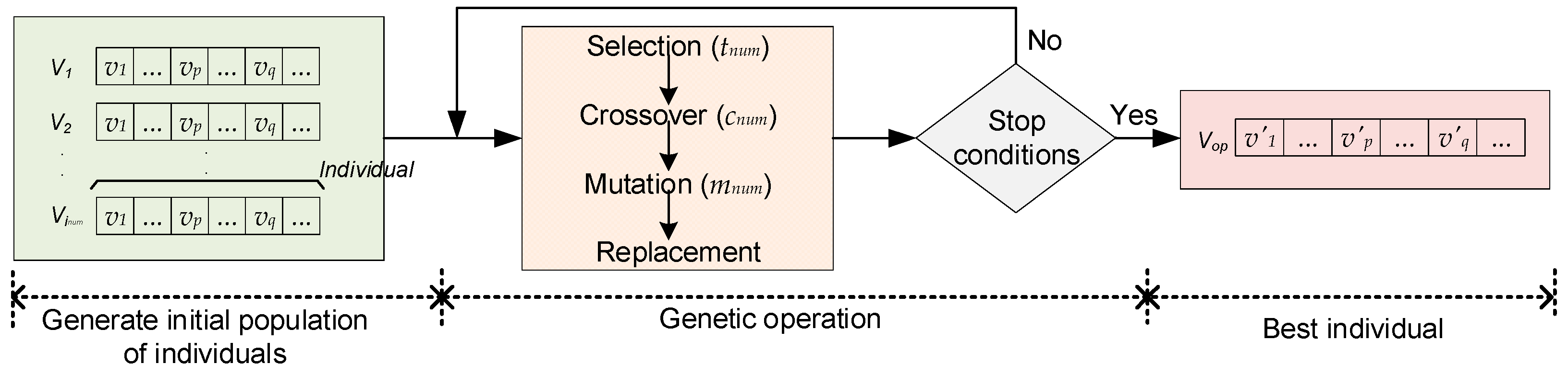
3.2. Optimization Algorithm Development

For a given problem, numerical algorithms, such as brute force or dynamic programming, can guarantee that one can find the global optimal result, as these algorithms calculate all possible solutions in the solution domain. Unfortunately, as the problem becomes more complex, the numerical algorithms become impractical due to large computation times. Therefore, a genetic algorithm has been developed in this work. As a metaheuristic method, the algorithm applies a heuristic random searching method using biological evolution. It includes an iterative process that operates based on a population of individuals. The process includes a few steps, such as initialization, evaluation, crossover, mutation, selection, and replacement, as shown in Figure 2. The algorithm uses heuristic guidance to search for the optimum, thereby significantly reducing the computation time with satisfactory suboptimal solutions.

Step 1: Initialization. As shown in the process below, to form the initial generation, the genetic algorithm firstly produces a random population of individuals (i_num). Each individual represents a potential solution to the optimization problem. The number of the individual numbers is recommended at 100 in this work [14].

(1)

When i = 1, the algorithm generates a vector V₁ to represent a single solution.

(2)

Let i = i + 1; the algorithm generates another vector V_i.

(3)

Repeat (2) until i > i_num to form the full generation. The algorithm then moves to Step 2 below.

Step 2: Evaluation. All the produced solutions need to be evaluated to identify their performance to the given problem.

(1)

Each solution will be used to produce a full-day timetable.

(2)

The full-day timetable will be imported to a train simulator to calculate the synchronized groups, overlapping time, train regenerative energy and full-day energy usage.

$$EVALUATION\left(V\right)=g\left(I{T}_{set},S{T}_{set}\right)$$

(4)

(3)

The solution with the smallest energy consumption represents the best individual. Then, it moves to Step 3 below.

Step 3: Genetic Operation. A genetic operation is introduced to choose appropriate individuals for producing new individuals to form the next generation. The operation contains different phases, including selection, crossover, mutation and replacement. In the selection phase, the top-ranking individuals (e.g., t_num = 10) will be retained for the next generation. In the crossover and mutation phase, the following individuals (e.g., c_num = m_num = 40) will be chosen for the crossover and mutation [15].

(1)

When i = 1, the algorithm produces a vector V′ = EVALUATION(V_i).

(2)

Let i = i + 1; the algorithm repeats the above process and generates $V_i^{\prime }$ until i > t_num. The program then moves to the crossover operation.

(3)

When j = 1, the algorithm chooses one element from two individuals and exchanges the elements with each other randomly. Assuming the individuals $V_{\alpha } =(v_1,\dots ,v_p,\dots ,v_q,\dots )$ and $V_{\beta } = (v_1^{\prime },\dots ,v_p^{\prime }, \dots ,v_q^{\prime },\dots )$, the elements p and q are chosen. After the crossover operation, the new individuals will look as $V_{\alpha }^{\prime } = (v_1,\dots ,v_p^{\prime },\dots ,v_q^{\prime },\dots )$ and $V_{\beta }^{\prime } = (v_1^{\prime },\dots , v_p,\dots ,v_q,\dots )$.

(4)

Let j = j + 2; the algorithm repeats the process above until j > c_num. The program then moves to the mutation operation.

(5)

When k = 1, the algorithm chooses one element from an individual and replaces it with a random value, which meets all the constraints in Equations (2) and (3). For instance, assuming the individual V_γ = (v₁, … v_s, …), the element s is selected. After the mutation operation, the new individual will look as $V_{\gamma }^{\prime } = (v_1,\dots v_s^{\prime },\dots )$.

(6)

Let k = k + 1; the genetic algorithm repeats the process above until k > m_num.

Step 4: Replacement. In the replacement phase, the algorithm will produce random individuals to replace the remaining individuals (e.g., r_num = 10) in EVALUATION(V);

(1)

When l = 1, the existing V_l is replaced by $V_l^{\prime }$, which is produced randomly by the algorithm and meets all constraints in Equations (2) and (3).

(2)

Let l = l + 1; the algorithm repeats the process above until l > r_num.

Step 5: Assembling. After the genetic operations, the produced individuals will be formed into a new generation.

$$\begin{array}{c}{V}^{\prime }=\left[V_i^{\prime },\dots .,V_{i+t_{num}}^{\prime },\dots ,V_{i+t_{num}+c_{num},}^{\prime },\dots V_{i+t_{num}+c_{num}+m_{num},}^{\prime },\dots V_{i+t_{num}+c_{num}+m_{num}+r_{num},}^{\prime }\dots ,V_{i_{num}}^{\prime }\right]\end{array}$$

(5)

Step 6: Termination. The new generation will be evaluated to identify their performance to the given problem from Step 2 above. The iteration will continue until the termination condition is matched (e.g., the generations number exceeds 100).

4. Metro Line Trial Test

4.1. Trial Test Introduction

A timetable optimization has been introduced in the previous chapters. It is important to apply the optimization result in a trial test to verify its performance and evaluate its reliability. In this work, a trial test was arranged on one of the metro lines in Guangzhou city, China. It is an urban metro line connecting the city center to suburban areas. The line is approximately 17 km long, with 7 intermediate stations. The single journey time is 45 min and the turn-over times at the terminal stations are 135 s and 145 s, respectively. The station dwelling times at the intermediate stations are between 35 and 45 s depending on the passenger flow.

A total of 144 train services are provided every day and 45 services operate during the peak-time hours, with 3 min service intervals. In the off-peak time hours, the service interval increases to 8 min. The interval time is designed based on the up-to-date passenger demand and can be re-scheduled every 4 months in practice. Therefore, this line was chosen for the trial test.

Table 2. The scheduled inter-station journey times.

Down Direction			Up Direction
Dwelling Time, Seconds	Inter-Station Journey Time, Seconds	Station Number	Inter-Station Journey Time, Seconds	Dwelling Time, Seconds
Turnover at the terminal station: 145 s
90	225	1	0	50
35	154	2	295	35
40	162	3	155	40
35	139	4	182	35
45	120	5	142	45
35	143	6	120	35
35	133	7	144	35
35	90	8	130	35
50	0	9	90	90
		Turnover at the terminal station: 135 s

and

Table 3. Scheduled service intervals and optimal service intervals.

Service Pattern for the Whole Day	Number of Services	Service Interval (mm:ss)
		Scheduled Timetable	Optimal Timetable
Peak-shift time	6	05:54 to 09:35	05:54 to 09:35
Morning peak-time	20	05:16	05:22 (+6 s)
Peak-shift time	1	06:40	06:40
Morning off-peak time	58	08:20	08:17 (−3 s)
Peak-shift time	1	05:40	05:40
Evening peak-time	25	05:16	05:22 (+6 s)
Peak-shift time	1	05:20	05:20
Evening off-peak time	28	08:20	08:17 (−3 s)
Peak-shift time	2	09:45 to 09:55	09:45 to 09:55
Total time:	144	66,228 s	66,240 s
Total braking synchronized time:		115,232	123,373

show the scheduled inter-section journey times and service intervals of the line.

Table 4. Train characteristics.

Subjects	Value
Rolling stock mass (tonne)	204
Maximum passenger load (tonne)	127
Power supply	DC 1500 V
Maximum tractive power (kW)	3700
Maximum braking power (kW)	3900
Rotary allowance	0.08
Tractive force (kN)	290
Braking force (kN)	350
Train formation	EMU 4M2T (4 motor cars, 2 trailer cars)
Train length (meter)	118
Top operational speed (km/h)	80

shows the train traction system characteristics. The train is equipped with a regenerative braking system with the maximum traction power and regenerative power at 3700 kW. The train tare mass is 204 tonnes and the top operational speed is 80 km/h. The passenger load is changing depending on the passenger flow. The train uses a DC 1500 V third-rail power supply system. The total train length is 118 m with 6 carriages. The train can be controlled by a human driving system or an automatic train operation system.

Table 3 shows the proposed optimal service intervals calculated by the developed algorithm with the constraints requested by the metro operator. The morning and evening peak-time service interval is increased by 6 s from 5:16 to 5:22, and the off-peak time service interval is reduced by 3 s. The difference between the whole day operation time is only 12 s, which is accepted by the operator. Furthermore, when using the optimal timetable, the total synchronized time is increased from 115,232 to 123,373, compared with the number using the scheduled timetable. The improved synchronized time can improve the utilization of the regenerative braking energy, and thus reduce the maximum power demand and energy usage on the line.

The trial test was arranged in the following three steps:

(1)

The optimal timetable was submitted to the operation department of the metro operator for approval, along with a trial test plan, which shows the test process, and the potential impact on the network operation.

(2)

Before the trial test, the staff from the operation department shall import the optimal timetable into the traffic management system (TMS). All the trains (with automatic train operation systems or human drivers) in the network shall operate following the new arrangement.

(3)

The whole-day train energy usage results from the trial test shall be compared with the data on a different day using the scheduled timetable (but the day of the week remains the same, e.g., Wednesday vs. Wednesday). To reduce any uncertainty, the test was arranged on a workday, rather than at weekends. This is because the passenger flow at the weekends may change significantly due to events or weather.

As the first trial test, to reduce the test complexity and minimize the impact of the change, the optimal timetable must meet the constraints given by the metro operator. For example, the changes in the service intervals must be within 5 s.

4.2. Results and Discussion

It is important to note that all the train running data are recorded using the onboard train monitoring recorder (OTMR), which is a device that records data about the train performance in response to the driver’s controls, including the time, position, tractive power, etc. Therefore, all the results presented in

Table 5. Comparison between the optimal timetable trial test and normal operation.

TCMS Output Data	Normal Operation Day (with Scheduled Timetable)	Trail Test Day (with Optimal Timetable)
Operation time	18.4 h	18.4 h
Total energy usage	51,767 kWh	50,649 kWh (−2.2%)
Train tractive energy usage	64,187 kWh	64,030 kWh (−0.2%)
Auxiliary energy usage	11,428 kWh	11,442 kWh (+0.1%)
Train regenerative braking energy usage	23,848 kWh	24,823 kWh (+4.1%)

are real-world data, rather than simulations.

In Table 5, the energy consumption and journey time are compared with the data captured on the other day using the scheduled timetable. It can be found that after applying the optimal timetable, the whole day journey time is not changed, which proves that the optimum timetable did not bring a significant impact on the train network. Furthermore, the differences in the train tractive energy usage and auxiliary energy usage are very small (within 0.2%), which means the passenger flow demand on these two days is similar. It can be observed from the table that the whole-day train regenerative braking energy utilization is increased by 4.1% from 23,848 kWh to 24,823 kWh. This shows that by implementing the optimal timetable, the efficiency of the regenerative braking system can be improved as the trains are operating with a more advanced energy utilization strategy. Such an improvement helps to reduce the total network energy consumption from 51,767 kWh to 50,649 kWh, without affecting the passenger flow.

In practice, the timetable of this metro line is reviewed every season and can be re-designed if necessary (for example, if the passenger flow demand is changed). The energy reduction from the trial test meets the requirements of the metro operator. Therefore, the optimal timetable can be permanently applied to the network for daily services. Furthermore, as the first trial test, the existing algorithm only optimized the service interval. The result can be further improved if other variables, such as the dwelling time, can be considered in the optimization.

5. Conclusions

In this paper, a timetable optimization and trial test work have been presented. The article has firstly introduced a train kinematics model to develop a train motion simulation. After this, an optimization algorithm has been proposed to reach the full potential of the train regenerative braking system and maximize the utilization of the regenerative braking energy. A trial test was carried out on a metro line for a whole day to verify the performance and practicability of the optimization results. All the trains running on the network during the trial test are required to operate in accordance with the optimal timetable. The energy consumption data were captured from the train onboard measurement systems and compared with the data from another day with the scheduled timetable.

The trial test shows that by implementing the optimal timetable, the utilization of the regenerative braking energy is improved, and the train energy usage can be reduced. The optimal timetable meets the constraints requested by the operator, which ensures the impact of the timetable rescheduling is minimized. The energy saving can be further improved if the metro operator liberalizes the optimization constraints when feasible in the future. The developed algorithm is shown to provide satisfactory results and meets the design requirements. However, the computation time of the existing optimization is relatively high (6 min). It is advised that the algorithm is more appropriate for implementation in off-line situations.

References

1. Kleftakis, V.A.; Hatziargyriou, N.D. Optimal control of reversible substations and wayside storage devices for voltage stabilization and energy savings in metro railway networks. IEEE Trans. Transp. Electrif. 2019, 5, 515–523. [Google Scholar] [CrossRef]
2. Hurt, G. FOI Request Detail, Energy Use. 2018. Available online: https://tfl.gov.uk/corporate/transparency/freedom-of-information/foi-request-detail?referenceId=FOI-1482-1819 (accessed on 1 May 2022).
3. Zhi, L. A Common Model for Railway Train Timetable Optimization. In Proceedings of the 2019 11th International Conference on Measuring Technology and Mechatronics Automation (ICMTMA), Qiqihar, China, 28–29 April 2019. [Google Scholar]
4. Parbo, J.; Nielsen, O.A.; Prato, C.G. User perspectives in public transport timetable optimisation. Transp. Res. Part C Emerg. Technol. 2014, 48, 269–284. [Google Scholar] [CrossRef] [Green Version]
5. Shuai, S.; Tao, T.; Xiang, L.; Ziyou, G. Optimization of multitrain operations in a subway system. Intell. Transp. Syst. IEEE Trans. 2014, 15, 673–684. [Google Scholar] [CrossRef]
6. Xin, Y.; Xiang, L.; Ziyou, G.; Hongwei, W.; Tao, T. A Cooperative Scheduling Model for Timetable Optimization in Subway Systems. Intell. Transp. Syst. IEEE Trans. 2013, 14, 438–447. [Google Scholar]
7. Watanabe, S.; Sato, Y.; Koseki, T.; Isobe, E.; Kawashita, J. Verification Test of Energy-Efficient Operations and Scheduling Utilizing Automatic Train Operation System. In Proceedings of the 2018 International Power Electronics Conference (IPEC-Niigata 2018-ECCE Asia), Niigata, Japan, 20–24 May 2018. [Google Scholar]
8. Montrone, T.; Pellegrini, P.; Nobili, P.; Longo, G. Energy consumption minimization in railway planning. In Proceedings of the 2016 IEEE 16th International Conference on Environment and Electrical Engineering (EEEIC), Florence, Italy, 7–10 June 2016. [Google Scholar]
9. López-López, Á.J.; Pecharromán, R.R.; Fernández-Cardador, A.; Cucala, A.P. Assessment of energy-saving techniques in direct-current-electrified mass transit systems. Transp. Res. Part C Emerg. Technol. 2014, 38, 85–100. [Google Scholar] [CrossRef]
10. Ning, L.; Li, Y.; Zhou, M.; Song, H.; Dong, H. A Deep Reinforcement Learning Approach to High-speed Train Timetable Rescheduling under Disturbances. In Proceedings of the 2019 IEEE Intelligent Transportation Systems Conference (ITSC), Auckland, New Zealand, 27–30 October 2019. [Google Scholar]
11. Hsi, P.-H.; Chen, S.-L. Electric load estimation techniques for high-speed railway (HSR) traction power systems. IEEE Trans. Veh. Technol. 2001, 50, 1260–1266. [Google Scholar] [CrossRef]
12. Loumiet, J.R.; Jungbauer, W.G. Train Accident Reconstruction and FELA and Railroad Litigation, 4th ed.; Lawyers & Judges Pub Co.: Tucson, AZ, USA, 2005; p. 767. [Google Scholar]
13. Hill, R. Electric railway traction. Part 1: Electric traction and DC traction motor drives. Power Eng. 1994, 8, 47–56. [Google Scholar] [CrossRef]
14. Cox, E. Fuzzy Modelling and Genetic Algorithms for Data Mining and Exploration, 1st ed.; Morgan Kaufmann: Burlington, MA, USA, 2005. [Google Scholar]
15. Rexhepi, A.; Maxhuni, A.; Dika, A. Analysis of the impact of parameters values on the Genetic Algorithm for TSP. Int. J. Comput. Sci. Issues 2013, 10, 158. [Google Scholar]
Figure 1. Regenerative braking power utilization.
Energies 15 04879 g001
Figure 2. Flowchart of the GA.
Energies 15 04879 g002