
Tower Models for Power Systems Transients: A Review

 ,
,  and
and 
Abstract
:1. Introduction
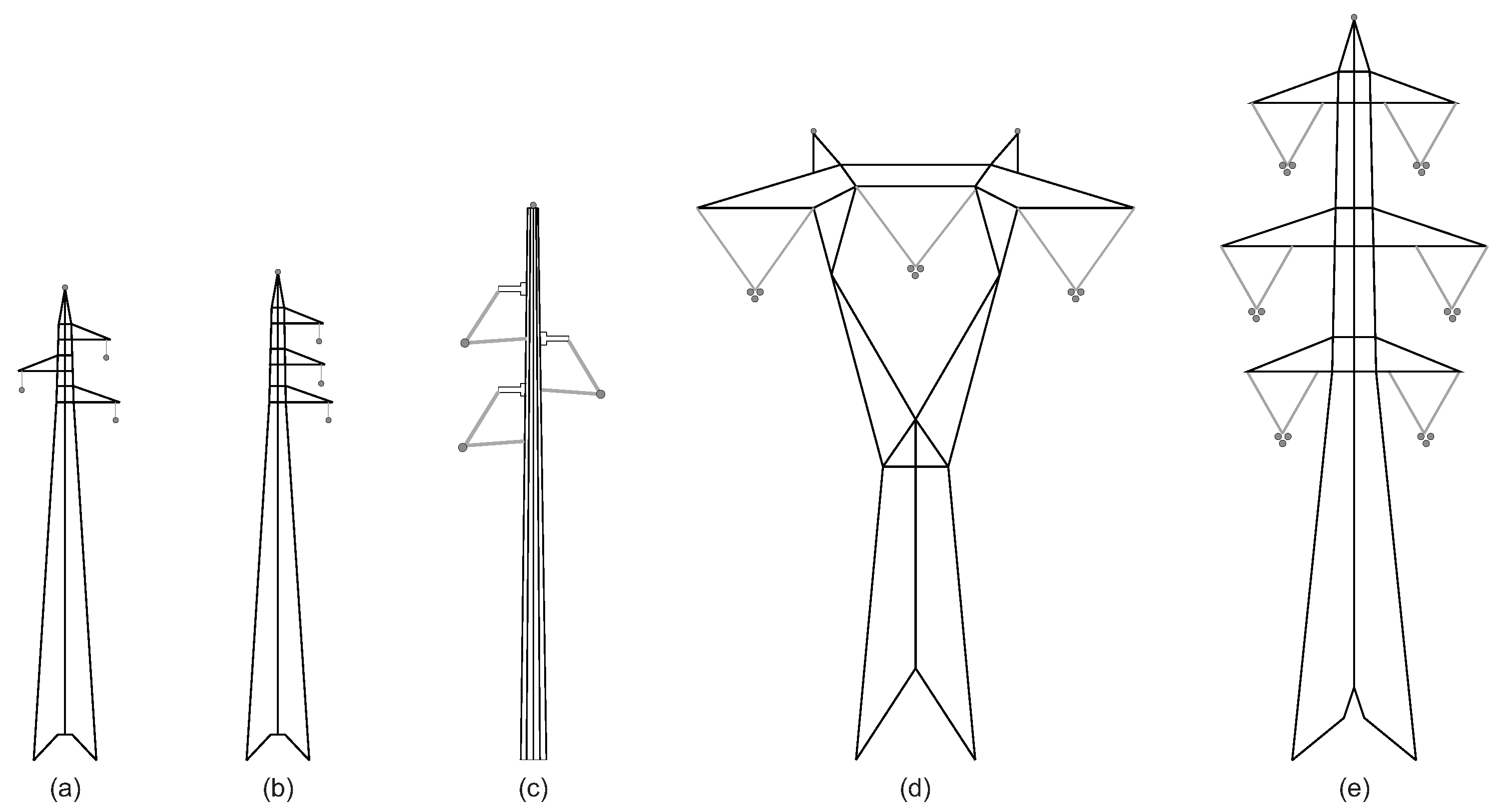
2. Towers for HV Applications and Common Conductors Arrangements
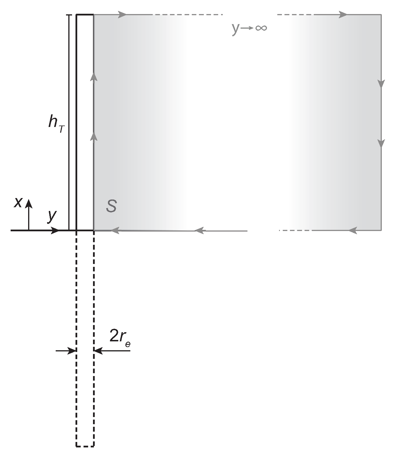
3. Definitions of Surge Impedance and Propagation Constant
Propagation Constant
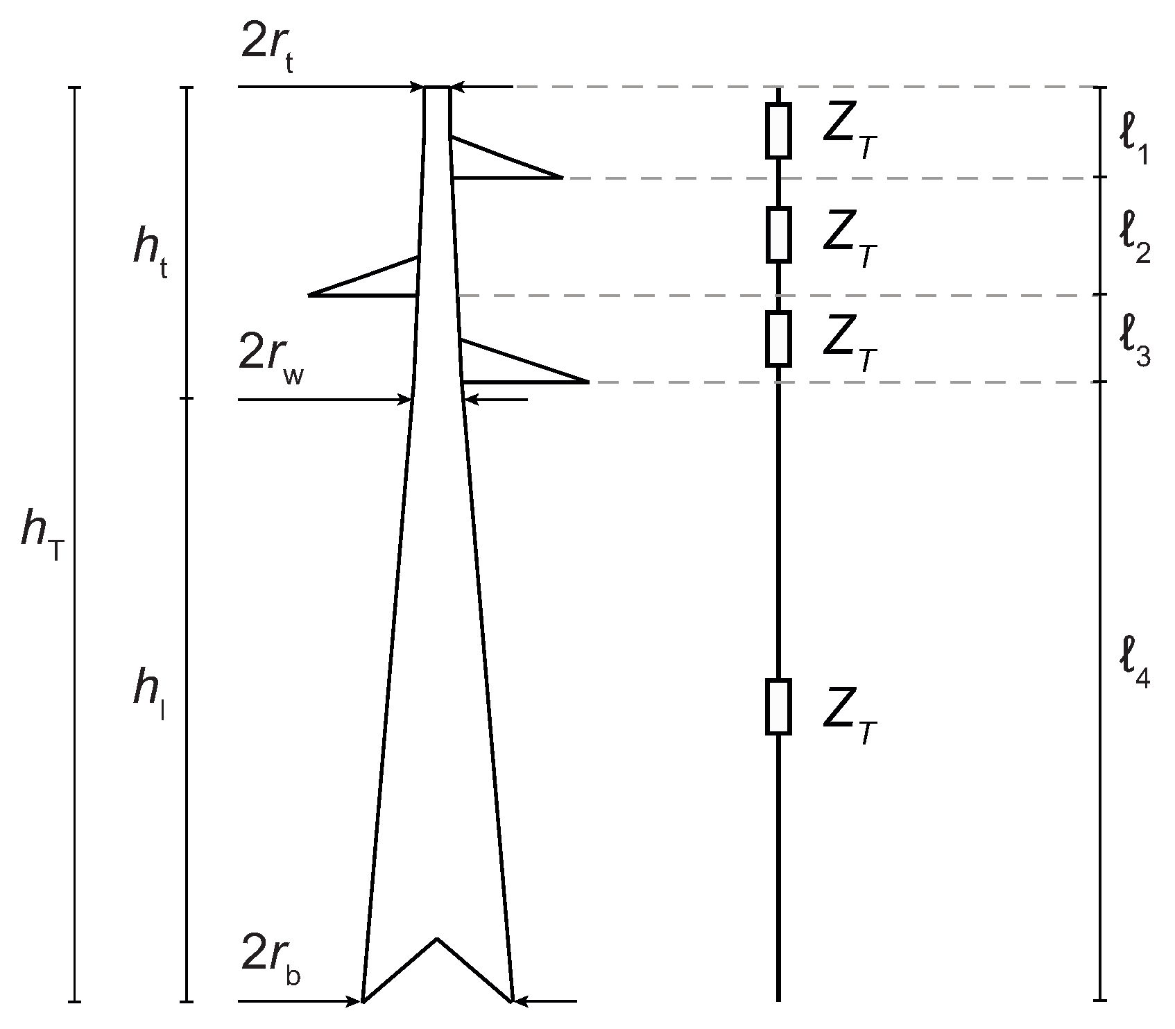
4. Tower Models
4.1. Lossless Uniform Transmission Line Models
4.1.1. Jordan Model
4.1.2. Wagner and Hileman Model
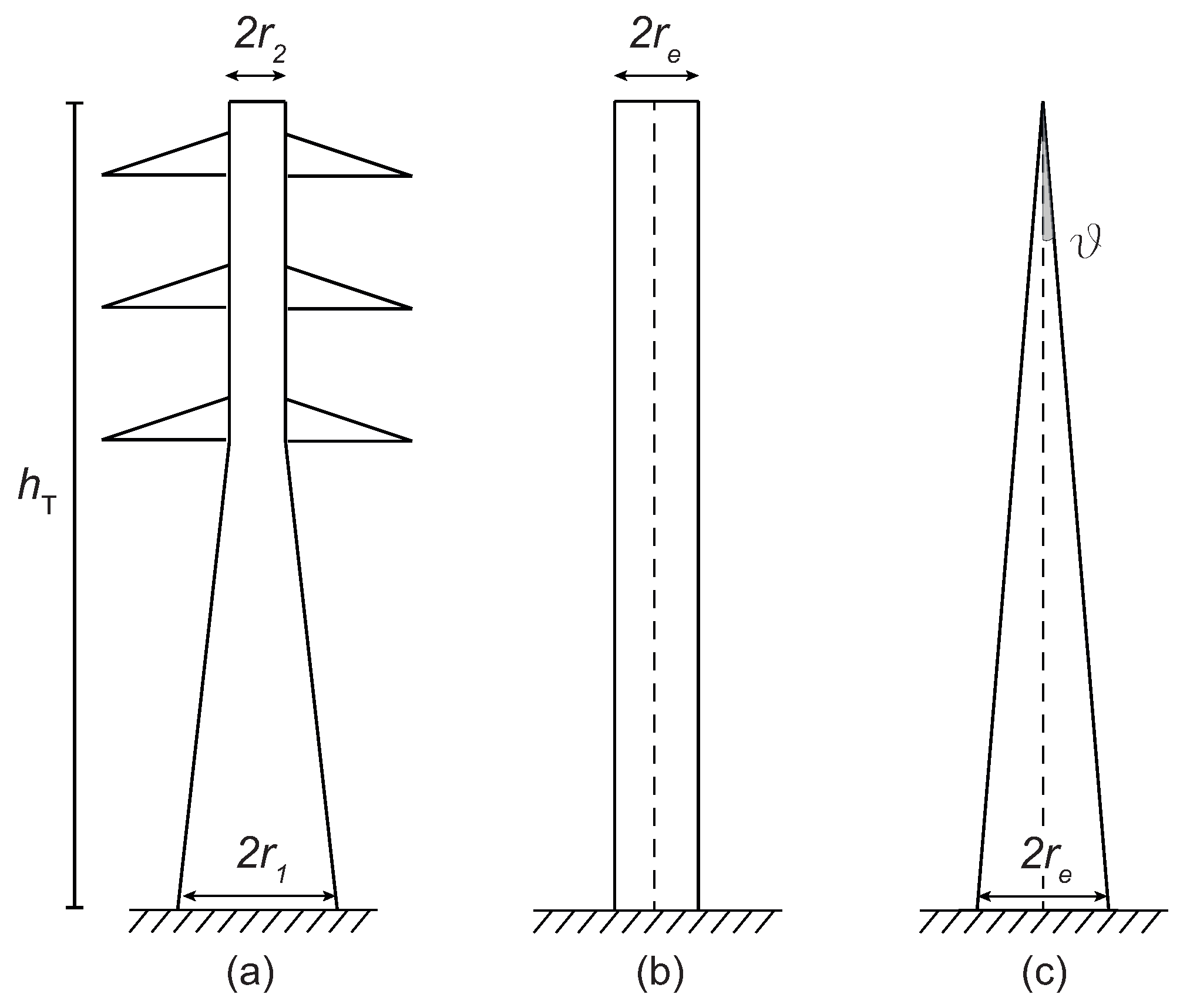
4.1.3. Sargent and Darveniza Model
4.1.4. Chisholm et al. Model
4.1.5. Remarks
4.2. Multiconductor Transmission Line Models
4.2.1. De Conti et al. Model
4.2.2. Hara and Yamamoto Model
4.2.3. Ametani et al. Model
4.3. Multistory Models
4.3.1. Ishii et al. Model
4.3.2. Baba et al. Model
4.3.3. Hashimoto et al. Model
4.3.4. Motoyama et al. Model
4.4. Non-Uniform Transmission Lines
4.4.1. Gutierrez et al. Model
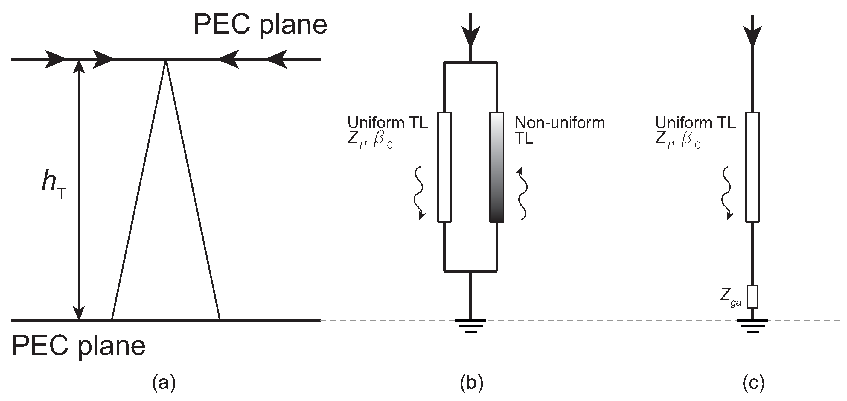
4.4.2. Saied et al. Model
4.4.3. Almeida and Correia De Barros Model
4.4.4. Other Models
5. Evaluation of the Tower Model Influence on Transients Studies
6. Conclusions and Final Remarks
- differences between downward and upward waves traveling along the tower;
- possible nonlinearities excited by the corona effect along the tower or by soil ionization;
- frequency-dependent behavior of the grounding grid at the tower base;
- non-TEM nature of the electromagnetic field along the tower.
Author Contributions
Funding
Informed Consent Statement
Data Availability Statement
Conflicts of Interest
References
- Hileman, A.R. Insulation Coordination For Power Systems; CRC Press: Boca Raton, FL, USA, 2018. [Google Scholar]
- IEC 60071-2022, TC 99; Insulation Co-Ordination and System Engineering of High Voltage Electrical Power Installations Above 1.0 kV AC and 1.5 kV DC. IEC: Geneva, Switzerland, 2022; pp. 1–901.
- IEEE Std C62.82.1-2010 (Revision of IEEE Std 1313.1-1996); IEEE Standard for Insulation Coordination–Definitions, Principles, and Rules. IEC: Geneva, Switzerland, 2011; pp. 1–22.
- IEEE Std 1313.2-1999; IEEE Guide for the Application of Insulation Coordination. IEEE: New York, NY, USA, 1999; pp. 1–68.
- Stracqualursi, E.; Araneo, R.; Celozzi, S. The Corona Phenomenon in Overhead Lines: Critical Overview of Most Common and Reliable Available Models. Energies 2021, 14, 6612. [Google Scholar] [CrossRef]
- Stracqualursi, E.; Araneo, R.; Andreotti, A. The impact of different corona models on FD algorithms for the solution of multiconductor transmission lines equations. High Voltage 2021, 6, 822–835. [Google Scholar] [CrossRef]
- Stracqualursi, E.; Araneo, R.; Faria, J.B.; Andreotti, A. Protection of distribution overhead power lines against direct lightning strokes by means of underbuilt ground wires. Electr. Power Syst. Res. 2022, 202, 107571. [Google Scholar] [CrossRef]
- Stracqualursi, E.; Araneo, R.; Faria, J.B.; Andreotti, A. Application of the Transfer Matrix Approach to Direct Lightning Studies of Overhead Power Lines with Underbuilt Shield Wires—Part I: Theory. IEEE Trans. Power Del. 2022, 37, 1226–1233. [Google Scholar] [CrossRef]
- Stracqualursi, E.; Araneo, R.; Faria, J.B.; Andreotti, A. Application of the Transfer Matrix Approach to Direct Lightning Studies of Overhead Power Lines with Underbuilt Shield Wires—Part II: Simulation Results. IEEE Trans. Power Del. 2022, 37, 1234–1241. [Google Scholar] [CrossRef]
- Araneo, R.; Andreotti, A.; Brandão Faria, J.; Celozzi, S.; Assante, D.; Verolino, L. Utilization of underbuilt shield wires to improve the lightning performance of overhead distribution lines hit by direct strokes. IEEE Trans. Power Del. 2020, 35, 1656–1666. [Google Scholar] [CrossRef]
- Andreotti, A.; Araneo, R.; Mahmood, F.; Pierno, A. An accurate approach for the evaluation of the performance of overhead distribution lines due to indirect lightning. Electr. Power Syst. Res. 2020, 186, 106411. [Google Scholar] [CrossRef]
- Andreotti, A.; Araneo, R.; Mahmood, F.; Piantini, A.; Rubinstein, M. An Analytical Approach to Assess the Influence of Shield Wires in Improving the Lightning Performance due to Indirect Strokes. IEEE Trans. Power Deliv. 2020, 36, 1491–1498. [Google Scholar] [CrossRef]
- Stracqualursi, E.; Araneo, R. Transient impedance of grounding grids with different soil models. In Proceedings of the 2021 IEEE International Conference on Environment and Electrical Engineering and 2021 IEEE Industrial and Commercial Power Systems Europe (EEEIC/I&CPS Europe), Bari, Italy, 8–11 June 2021; pp. 1–6. [Google Scholar]
- Chowdhuri, P.; Li, S.; Yan, P. Rigorous analysis of back-flashover outages caused by direct lightning strokes to overhead power lines. IEE Proc. Gener. Transm. Distrib. 2002, 149, 58–65. [Google Scholar] [CrossRef]
- Silveira, F.H.; Visacro, S.; De Conti, A.; Mesquita, C.R.d. Backflashovers of Transmission Lines Due to Subsequent Lightning Strokes. IEEE Trans. Electromagn. Compat. 2012, 54, 316–322. [Google Scholar] [CrossRef]
- Silveira, F.H.; Visacro, S. Lightning performance of transmission lines: Impact of current waveform and front-time on backflashover occurrence. IEEE Trans. Power Del. 2019, 34, 2145–2151. [Google Scholar] [CrossRef]
- Silveira, F.H.; Almeida, F.S.; Visacro, S.; Zago, G.M.P. Influence of the current front time representation on the assessment of backflashover occurrence of transmission lines by deterministic and probabilistic calculation approaches. Electr. Power Syst. Res. 2021, 197, 107299. [Google Scholar] [CrossRef]
- Sindeband, M.; Sporn, P. Lightning and Other Experience with 132-kV. Steel Tower Transmission Lines, and its Bearing on Tower-Line Design from the Continuity of Service Standpoint. Trans. Am. Inst. Electr. Eng. 1926, 45, 770–790. [Google Scholar] [CrossRef]
- Bewley, L. Critique of Ground Wire Theory. Trans. Am. Inst. Electr. Eng. 1931, 50, 1–18. [Google Scholar] [CrossRef]
- Fortescue, C.; Fielder, F. Counterpoise tests at Trafford. Electr. Eng. 1934, 53, 1116–1123. [Google Scholar] [CrossRef]
- Jordan, C.A. Lightning computation for transmission line with overhead ground wires. Gen. Electr. Rev. 1934, 37, 180–186. [Google Scholar]
- Silveira, F.H.; Visacro, S.; Souza, R.E. Lightning performance of transmission lines: Assessing the quality of traditional methodologies to determine backflashover rate of transmission lines taking as reference results provided by an advanced approach. Electr. Power Syst. Res. 2017, 153, 60–65. [Google Scholar] [CrossRef]
- Almeida, F.S.; Silveira, F.H.; De Conti, A.; Visacro, S. Influence of tower modeling on the assessment of backflashover occurrence on transmission lines due to first negative lightning strokes. Electr. Power Syst. Res. 2021, 197, 107307. [Google Scholar] [CrossRef]
- Datsios, Z.; Mikropoulos, P. Effect of tower modelling on the minimum backflashover current of overhead transmission lines. In Proceedings of the 19th International Symposium on High Voltage Engineering (ISH), Pilsen, Czech Republic, 23–28 August 2015. [Google Scholar]
- Mikropoulos, P.N.; Tsovilis, T.E.; Datsios, Z.G.; Mavrikakis, N.C. Effects of simulation models of overhead transmission line basic components on backflashover surges impinging on GIS substations. In Proceedings of the 45th IEEE International Universities Power Engineering Conference UPEC2010, Cardiff, UK, 31 August–3 September 2010; pp. 1–6. [Google Scholar]
- Savic, M.S.; Savic, A.M. Substation Lightning Performance Estimation Due to Strikes Into Connected Overhead Lines. IEEE Trans. Power Del. 2015, 30, 1752–1760. [Google Scholar] [CrossRef]
- Huang, L.; Zhou, L.; Wu, T.; Hu, C.; Zhang, D.; Wang, D.; Chen, S. A distributed modelling method of the transmission tower and transient response analysis of lightning wave process. IET Gener. Transm. Distrib. 2021, 15, 3017–3031. [Google Scholar] [CrossRef]
- Grcev, L.; Rachidi, F. On tower impedances for transient analysis. IEEE Trans. Power Del. 2004, 19, 1238–1244. [Google Scholar] [CrossRef]
- Salarieh, B.; De Silva, H.M.J.; Gole, A.M.; Ametani, A.; Kordi, B. An Electromagnetic Model for the Calculation of Tower Surge Impedance Based on Thin Wire Approximation. IEEE Trans. Power Del. 2021, 36, 1173–1182. [Google Scholar] [CrossRef]
- Ametani, A.; Triruttanapiruk, N.; Yamamoto, K.; Baba, Y.; Rachidi, F. Impedance and Admittance Formulas for a Multistair Model of Transmission Towers. IEEE Trans. Electromagn. Compat. 2020, 62, 2491–2502. [Google Scholar] [CrossRef]
- Yamanaka, A.; Nagaoka, N.; Baba, Y. Circuit model of vertical double-circuit transmission tower and line for lightning surge analysis considering TEM-mode formation. IEEE Trans. Power Del. 2020, 35, 2471–2480. [Google Scholar] [CrossRef]
- Thang, T.H.; Baba, Y.; Nagaoka, N.; Ametani, A.; Takami, J.; Okabe, S.; Rakov, V.A. A Simplified Model of Corona Discharge on Overhead Wire for FDTD Computations. IEEE Trans. Electromagn. Compat. 2012, 54, 585–593. [Google Scholar] [CrossRef]
- Saito, M.; Ishii, M.; Miki, M.; Tsuge, K. On the Evaluation of the Voltage Rise on Transmission Line Tower Struck by Lightning Using Electromagnetic and Circuit-Based Analyses. IEEE Trans. Power Del. 2021, 36, 627–638. [Google Scholar] [CrossRef]
- Cao, J.; Du, Y.; Ding, Y.; Li, B.; Qi, R.; Zhang, Y.; Li, Z. Lightning Surge Analysis of Transmission Line Towers With a Hybrid FDTD-PEEC Method. IEEE Trans. Power Del. 2022, 37, 1275–1284. [Google Scholar] [CrossRef]
- Salarieh, B.; De Silva, H.J.; Kordi, B. Electromagnetic transient modeling of grounding electrodes buried in frequency dependent soil with variable water content. Electr. Power Syst. Res. 2020, 189, 106595. [Google Scholar] [CrossRef]
- Silva, B.P.; Visacro, S.; Silveira, F.H. HEM-TD: New Time-Domain Electromagnetic Model for Calculating the Lightning Response of Electric Systems and Their Components. IEEE Trans. Power Deliv. 2022, 1–9. [Google Scholar] [CrossRef]
- Salarieh, B.; Kordi, B. Full-wave black-box transmission line tower model for the assessment of lightning backflashover. Electr. Power Syst. Res. 2021, 199, 107399. [Google Scholar] [CrossRef]
- Zhang, Y.; Li, L.; Han, Y.; Ruan, Y.; Yang, J.; Cai, H.; Liu, G.; Zhang, Y.; Jia, L.; Ma, Y. Flashover Performance Test with Lightning Impulse and Simulation Analysis of Different Insulators in a 110 kV Double-Circuit Transmission Tower. Energies 2018, 11, 659. [Google Scholar] [CrossRef] [Green Version]
- De Conti, A.; Visacro, S.; Soares, A.; Schroeder, M.A.O. Revision, extension, and validation of Jordan’s formula to calculate the surge impedance of vertical conductors. IEEE Trans. Electromagn. Compat. 2006, 48, 530–536. [Google Scholar] [CrossRef]
- Slyunyaev, N.N.; Mareev, E.A.; Rakov, V.A.; Golitsyn, G.S. Statistical Distributions of Lightning Peak Currents: Why Do They Appear to Be Lognormal? J. Geophys. Res. Atmos. 2018, 123, 5070–5089. [Google Scholar] [CrossRef]
- Takahashi, H. Confirmation of the Error of Jordan’s Formula on Tower Surge Impedance. IEEJ Trans. Power Energy 1994, 114, 112–113. [Google Scholar] [CrossRef] [Green Version]
- Wagner, C.F.; Hileman, A.R. A New Approach to the Calculation or the Lightning Perrormance or Transmission Lines III—A Simplified Method: Stroke to Tower. AIEE Trans. Power Appar. Syst. 1960, 79, 589–603. [Google Scholar] [CrossRef]
- Sargent, M.A.; Darveniza, M. Tower Surge Impedance. IEEE Trans. Power Appl. Syst. 1969, PAS-88, 680–687. [Google Scholar] [CrossRef]
- Chisholm, W.A.; Chow, Y.L.; Srivastava, K.D. Surge response of transmission towers. Can. Electr. Eng. J. 1982, 7, 34–36. [Google Scholar] [CrossRef]
- Chisholm, W.A.; Chow, Y.L.; Srivastava, K.D. Travel Time of Transmission Towers. IEEE Trans. Power Appl. Syst. 1985, PAS-104, 2922–2928. [Google Scholar] [CrossRef]
- Rondon, D.; Vargas, M.; Herrera, J.; Montana, J.; Torres, H.; Camargo, M.; Jimenez, D.; Delgadillo, A. Influence of grounding system modeling on transient analysis of transmission lines due to direct lightning strike. In Proceedings of the 2005 IEEE Russia Power Tech, St. Petersburg, Russia, 27–30 June 2005; pp. 1–6. [Google Scholar]
- Saied, M.M.; AlFuhaid, A.S.; El-Shandwily, M.E. s-domain analysis of electromagnetic transients on nonuniform lines. IEEE Trans. Power Del. 1990, 5, 2072–2083. [Google Scholar] [CrossRef]
- Oufi, E.; AlFuhaid, A.; Saied, M. Transient analysis of lossless single-phase nonuniform transmission lines. IEEE Trans. Power Del. 1994, 9, 1694–1700. [Google Scholar] [CrossRef]
- Almeida, M.; De Barros, M.C. Tower modelling for lightning surge analysis using Electro-Magnetic Transients Program. IEE Proc.-Gener. Transm. Distrib. 1994, 141, 637–639. [Google Scholar] [CrossRef]
- Barros, M.T.C.D.; Almeida, M.E. Computation of electromagnetic transients on nonuniform transmission lines. IEEE Trans. Power Del. 1996, 11, 1082–1091. [Google Scholar] [CrossRef]
- Hara, T.; Yamamoto, O.; Hayashi, M.; Uenosono, C. Empirical formulas for surge impedance for single and multiple vertical conductors. IEEJ Trans. Power Energy 1990, B-110, 129–136. [Google Scholar] [CrossRef] [Green Version]
- Ametani, A.; Kasai, Y.; Sawada, J.; Mochizuki, A.; Yamada, T. Frequency-dependent impedance of vertical conductors and a multiconductor tower model. IEE Proc. Gener. Transm. Distrib. 1994, 141, 339–345. [Google Scholar] [CrossRef]
- Moreno, P.; Naredo, J.L.; Bermúdez, J.L.; Paolone, M.; Nucci, C.A.; Rachidi, F. Nonuniform transmission tower model for lightning transient studies. IEEE Trans. Power Del. 2004, 19, 490–496. [Google Scholar]
- Gutierrez, J.; Moreno, P.; Guardado, L.; Naredo, J. Comparison of transmission tower models for evaluating lightning performance. In Proceedings of the 2003 IEEE Bologna Power Tech Conference, Bologna, Italy, 23–26 June 2003; Volume 4. [Google Scholar]
- Ishii, M.; Kawamura, T.; Kouno, T.; Ohsaki, E.; Shiokawa, K.; Murotani, K.; Higuchi, T. Multistory transmission tower model for lightning surge analysis. IEEE Trans. Power Del. 1991, 6, 1327–1335. [Google Scholar] [CrossRef]
- Baba, Y.; Ishii, M. Tower models for fast-front lightning currents. IEEJ Trans. Power Energy 2000, 120, 18–23. [Google Scholar] [CrossRef] [Green Version]
- Hashimoto, S.; Baba, Y.; Nagaoka, N.; Ametani, A.; Itamoto, N. An equivalent circuit of a transmission-line tower struck by lightning. In Proceedings of the 2010 30th IEEE International Conference on Lightning Protection (ICLP), Cagliari, Italy, 13–17 September 2010; pp. 1–6. [Google Scholar]
- Motoyama, H.; Shinjo, K.; Matsumoto, Y.; Itamoto, N. Observation and analysis of multiphase back flashover on the Okushishiku test transmission line caused by winter lightning. IEEE Trans. Power Del. 1998, 13, 1391–1398. [Google Scholar] [CrossRef]
- Yamada, T.; Mochizuki, A.; Sawada, J.; Zaima, E.; Kawamura, T.; Ametani, A.; Ishii, M.; Kato, S. Experimental evaluation of a UHV tower model for lightning surge analysis. IEEE Trans. Power Del. 1995, 10, 393–402. [Google Scholar] [CrossRef]
- Noda, T. A tower model for lightning overvoltage studies based on the result of an FDTD simulation. IEEJ Trans. Power Energy 2007, 127, 379–388. [Google Scholar] [CrossRef] [Green Version]
- Gatta, F.M.; Geri, A.; Lauria, S.; Maccioni, M. Generalized pi-circuit tower grounding model for direct lightning response simulation. Electr. Power Syst. Res. 2014, 116, 330–337. [Google Scholar] [CrossRef]
- Alemi, M.R.; Sheshyekani, K. Wide-Band Modeling of Tower-Footing Grounding Systems for the Evaluation of Lightning Performance of Transmission Lines. IEEE Trans. Electromagn. Compat. 2015, 57, 1627–1636. [Google Scholar] [CrossRef]
- Schroeder, M.A.O.; de Barros, M.T.C.; Lima, A.C.S.; Afonso, M.M.; Moura, R.A.R. Evaluation of the impact of different frequency dependent soil models on lightning overvoltages. Electr. Power Syst. Res. 2018, 159, 40–49. [Google Scholar] [CrossRef]
- Visacro, S.; Silveira, F.H. The Impact of the Frequency Dependence of Soil Parameters on the Lightning Performance of Transmission Lines. IEEE Trans. Electromagn. Compat. 2015, 57, 434–441. [Google Scholar] [CrossRef]
- Feng, Z.; Wen, X.; Tong, X.; Lu, H.; Lan, L.; Xing, P. Impulse Characteristics of Tower Grounding Devices Considering Soil Ionization by the Time-Domain Difference Method. IEEE Trans. Power Del. 2015, 30, 1906–1913. [Google Scholar] [CrossRef]
- Lings, R. EPRI AC Transmission Line Reference Book: 200 kV and Above, 3rd ed.; Electric Power Research Institute: Palo Alto, CA, USA, 2005. [Google Scholar]
- LaForest, J.J. Transmission Line Reference Book: 345 kV and Above; Electric Utility Systems Engineering Department: Schenectady, NY, USA, 1981. [Google Scholar]
- Menemenlis, C.; Chun, Z.T. Wave Propagation on Nonuniform Lines. IEEE Trans. Power Appl. Syst. 1982, PAS-101, 833–839. [Google Scholar] [CrossRef]
- CIGRE TB 549; Lightning Parameters for Engineering Applications. CIGRE: Paris, France, 2013; 118p.
- Javor, V.; Lundengård, K.M.; Rančić, M.P.; Silvestrov, S. Analytical representation of measured lightning currents and its application to electromagnetic field estimation. IEEE Trans. Electromagn. Compat. 2017, 60, 1415–1426. [Google Scholar] [CrossRef]
- Uman, M.A.; Krider, E.P. A review of natural lightning: Experimental data and modeling. IEEE Trans. Electromagn. Compat. 1982, EMC-24, 79–112. [Google Scholar] [CrossRef]
- Kawai, M. Studies of the surge response on a transmission line tower. IEEE Trans. Power Appl. Syst. 1964, 83, 30–34. [Google Scholar] [CrossRef]
- Breuer, G.; Schultz, A.; Schlomann, R.; Price, W. Field studies of the surge response of a 345-kV transmission tower and ground wire. Trans. Am. Inst. Electr. Eng. Part III Power Appar. Syst. 1958, 76, 1392–1396. [Google Scholar] [CrossRef]
- Motoyama, H.; Matsubara, H. Analytical and experimental study on surge response of transmission tower. IEEE Trans. Power Del. 2000, 15, 812–819. [Google Scholar] [CrossRef]
- Chisholm, W.A.; Chow, Y.; Srivastava, K.D. Lightning Surge Response Of Transmission Towers. IEEE Trans. Power Appl. Syst. 1983, PAS-102, 3232–3242. [Google Scholar] [CrossRef]
- Motoyama, H.; Kinoshita, Y.; Nonaka, K. Experimental study on lightning surge response of 500-kV transmission tower with overhead lines. IEEE Trans. Power Del. 2008, 23, 2488–2495. [Google Scholar] [CrossRef]
- Velasco, J.A.M. Power System Transients: Parameter Determination; CRC Press: Boca Raton, FL, USA, 2010. [Google Scholar]
- Lundholm, R.; Finn, R.B.; Price, W.S. Calculation of Transmission Line Lightning Voltages by Field Concepts. Trans. Am. Inst. Electr. Eng. Part III Power Appar. Syst. 1957, 76, 1271–1281. [Google Scholar] [CrossRef]
- Anderson, J.G.; Hagenguth, J.H. Magnetic Fields Around a Transmission Line Tower. Trans. Am. Inst. Electr. Eng. Part III Power Appar. Syst. 1958, 77, 1644–1649. [Google Scholar] [CrossRef]
- Rothwell, E.J.; Cloud, M.J. Electromagnetics; CRC Press: Boca Raton, FL, USA, 2018. [Google Scholar]
- Whitehead, J.T.; Chisholm, W.A.; Anderson, J.; Clayton, R.; Elahi, H.; Eriksson, A.; Grzybowski, S.; Hileman, A.; Janischewskyj, W.; Longo, V.; et al. Estimating lightning performance of transmission line 2–Updates to analytical models. IEEE Trans. Power Del. 1993, 8, 1254–1267. [Google Scholar]
- Baba, Y.; Rakov, V.A. On the interpretation of ground reflections observed in small-scale experiments simulating lightning strikes to towers. IEEE Trans. Electromagn. Compat. 2005, 47, 533–542. [Google Scholar] [CrossRef]
- Bermudez, J.L.; Gutierrez, J.; Chisholm, W.; Rachidi, F.; Paolone, M.; Moreno, P. A reduced-scale model to evaluate the response of tall towers hit by lightning. In Proceedings of the SICEL’2001, Bogotà, Colombia, 2001. [Google Scholar]
- Hara, T.; Yamamoto, O. Modelling of a transmission tower for lightning-surge analysis. IEE Proc. Gener. Transm. Distrib. 1996, 143, 283–289. [Google Scholar] [CrossRef] [Green Version]
- Deri, A.; Tevan, G.; Semlyen, A.; Castanheira, A. The Complex Ground Return Plane a Simplified Model for Homogeneous and Multi-Layer Earth Return. IEEE Trans. Power Appl. Syst. 1981, 100, 3686–3693. [Google Scholar] [CrossRef]
- Ueda, T.; Ito, T.; Watanabe, H.; Funabashi, T.; Ametani, A. A comparison between two tower models for lightning surge analysis of 77 kV system. In Proceedings of the PowerCon 2000, 2000 IEEE International Conference on Power System Technology. Proceedings (Cat. No. 00EX409), Perth, WA, Australia, 4–7 December 2000; Volume 1, pp. 433–437. [Google Scholar]
- Ishii, M.; Baba, Y. Numerical electromagnetic field analysis of tower surge response. IEEE Trans. Power Del. 1997, 12, 483–488. [Google Scholar] [CrossRef]
- Baha, Y.; Ishii, M. Numerical electromagnetic field analysis on lightning surge response of tower with shield wire. IEEE Trans. Power Del. 2000, 15, 1010–1015. [Google Scholar] [CrossRef]
- Baba, Y.; Ishii, M. Numerical electromagnetic field analysis on measuring methods of tower surge impedance. IEEE Trans. Power Del. 1999, 14, 630–635. [Google Scholar] [CrossRef]
- Motoyama, H.; Kinoshita, Y.; Nonaka, K.; Baba, Y. Experimental and Analytical Studies on Lightning Surge Response of 500-kV Transmission Tower. IEEE Trans. Power Del. 2009, 24, 2232–2239. [Google Scholar] [CrossRef]
- Paul, C.R. Analysis of Multiconductor Transmission Lines; John Wiley and Sons: Hoboken, NJ, USA, 2008. [Google Scholar]
- Guo, X.; Fu, Y.; Yu, J.; Xu, Z. A non-uniform transmission line model of the ±1100 kV UHV tower. Energies 2019, 12, 445. [Google Scholar] [CrossRef] [Green Version]
- Yamanaka, A. Lightning Surge Analysis of Transmission Lines Using Circuit Models Considering Electromagnetic Phenomena. Ph.D. Thesis, Doshisha University, Kyoto, Japan, 2021. [Google Scholar]
- Yamanaka, A.; Nagaoka, N.; Baba, Y. Circuit Model of an Overhead Transmission Line Considering the TEM-Mode Formation Delay. IEEJ Trans. Electr. Electron. Eng. 2021, 16, 888–895. [Google Scholar] [CrossRef]
- Gatta, F.M.; Geri, A.; Lauria, S.; Maccioni, M.; Palone, F. Lightning Performance Evaluation of Italian 150 kV Sub-Transmission Lines. Energies 2020, 13, 2142. [Google Scholar] [CrossRef]
- Datsios, Z.G.; Stracqualursi, E.; Araneo, R.; Mikropoulos, P.N.; Tsovilis, T.E. Estimation of the Minimum Backflashover Current and Backflashover Rate of a 150 kV Overhead Transmission Line: Frequency and Current-Dependent Effects of Grounding Systems. In Proceedings of the 2022 IEEE International Conference on Environment and Electrical Engineering and 2022 IEEE Industrial and Commercial Power Systems Europe (EEEIC/I&CPS Europe), Prague, Czech Republic, 2022. submitted. [Google Scholar]
- Conti, A.D.; Visacro, S. Analytical Representation of Single- and Double-Peaked Lightning Current Waveforms. IEEE Trans. Electromagn. Compat. 2007, 49, 448–451. [Google Scholar] [CrossRef]
- Gamerota, W.R.; Elismé, J.O.; Uman, M.A.; Rakov, V.A. Current Waveforms for Lightning Simulation. IEEE Trans. Electromagn. Compat. 2012, 54, 880–888. [Google Scholar] [CrossRef]


| Authors | Ref. | Experimental Arrangement | Height | |
|---|---|---|---|---|
| Breuer et al. | [73] | HV tower, vertical conductors | 51 44 | 0.95–0.96 |
| Ishii et al. | [55] | HV tower | 62.8 | ≃1 |
| Kawai et al. | [72] | HV tower | 26–214 | 0.7–0.88 |
| Motoyama et al. | [74] | Reduced-scale model HV tower UHV tower | 3 48.2 120 | 0.8–0.87 |
| Chisholm et al. | [45] | Reduced-scale smooth cone | 0.4 | ≃1 |
| Chisholm et al. | [75] | HV towers | 25.5–57.0 | 0.96–1 |
| Motoyama et al. | [76] | HV tower | 89.5–94.5 | 0.85–0.9 |
| Noda | [60] | HV tower | 77 |
| Model | Type | Main Features | Equivalent | Soil Effect |
|---|---|---|---|---|
| Jordan [21,39,41] | Lossless uniform TL | Based on magnetostatics principles and low-frequency approximations. | Cylindrical | × |
| Wagner and Hileman [42] | Lossless uniform TL | Derived in the time domain by loop-voltage method and Kirchhoff’s current law. The characteristic impedance is assumed equal to the value attained by the transient surge impedance at . | Cylindrical | × |
| Sargent and Darveniza [43] | Lossless uniform TL | Analysis developed in the time domain. Characteristic impedance computed as the value attained at by the ratio of the tower top voltage (integral of the electric field, neglecting the effect of the scalar electric potential) over the injected current. | Cylindrical Conical | × |
| Chisholm et al. [44,45] | Lossless uniform TL | Accounting for horizontal direction of current injection at the tower top. Derived by application of theory of biconical TLs. | Cylindrical Conical | × |
| De Conti et al. [39] | Lossless MTL | MTL model based on magnetostatics principles and per unit length inductances computation. | Cylindrical | × |
| Hara and Yamamoto [51] | Lossless TL | Cascade of parallel lossless TLs (with empirical characteristic impedances) accounting for the legs and bracing. The four main legs of the tower are reduced to a simple TL through an equivalent radius. Additional lossless, horizontal TLs account for the arms. | Cylindrical | × |
| Ametani et al. [52] | MTL | Computation of a potential coefficient matrix for each tower section accounting for current images with respect to a reference plane at complex depth. The tower is modeled by a cascade of multiconductor (or single-conductor with an equivalent radius) TLs. | Cylindrical | ✓ |
| Ishii et al. [55] Baba et al. [56] | Multistory model | Cascade of lossless TLs and damping resistive-inductive elements. Values of the characteristic impedances are derived empirically. | - | × |
| Hashimoto et al. [57] | Multistory model | Cascade of TLs and damping resistive-inductive elements, with an additional capacitance-to-ground at the tower top. Values of the characteristic impedances and lumped elements are derived to reproduce available experimental data for the system consisting in a tower equipped with power-line conductors. | - | × |
| Model | Type | Main Features | Equivalent | Soil Effect |
|---|---|---|---|---|
| Motoyama et al. [58] | Multistory model | Cascade of TLs and damping resistive-inductive elements. Values of the characteristic impedances are derived empirically. | - | × |
| Gutierrez et al. [53] | Non-uniform TL | Non-uniform MTL (or single conductor equivalent) with characteristic impedances given by the ratio of the voltage (computed as the integral of the electric field in the polar direction produced by a bipolar antenna with vertex lying on a reference plane at complex depth) and the source current. | Cylindrical | ✓ |
| Saied et al. [47] | Lossless non-uniform TL | Cylindrical exponential TL model, with progressive-dependent characteristic impedance (starting from assumed values at relevant heights). | Cylindrical | × |
| Almeida and Correia de Barros [49] | Non-uniform TL | Progressive-dependent characteristic impedance (starting from assumed values at the tower top and base). Propagation assessed by means of FDTD methods and possible inclusion of frequency-independent per unit length losses. | Cylindrical | × |
| Model | Story 1 | Story 2 | Story 3 | Story 4 |
|---|---|---|---|---|
| Ishii et al. [55] | | | | |
| Baba et al. [56] | | , | , | , , |
| Motoyama et al. [58] | | | | |
| Yamada et al. [59] | | | | |
| Model | Story 1 m | Story 2 m | Story 3 m | Story 4 m |
|---|---|---|---|---|
| Ishii et al. [55] | H | H | H | H |
| Baba et al. [56] | H | H | H H | |
| Motoyama et al. [58] | H | H | H | H |
| Yamada et al. [59] | H | H | H | H |
| Tower (a) | Tower (b) | ||
|---|---|---|---|
| [m] | 30.2 | 47.4 | |
| [m] | 2.0 | 3.95 | |
| [m] | 0.55 | 1.4 | |
| [m] | 0.4 | 2.0 | |
| [m] | 3.25 | 5.3 | |
| [m] | 2.0 | 9.2 | |
| [m] | 2.0 | 8 | |
| [m] | 22.95 | 24.9 | |
| [m] | 0.25 | 0.5 | |
| [cm] | 6.0 | 9.0 |
| Type | ||||||||
|---|---|---|---|---|---|---|---|---|
| [m] | [m] | [m] | [m] | [mm] | [m] | - | [] | |
| MT2 | 1.0 | 1.0 | 0.8 | 2.0 | 14.0 | 150 | 20 | 15.3 |
| MT4 | 12.0 | 1.0 | 1.0 | 3.95 | 14.0 | 600 | 20 | 18.7 |
Publisher’s Note: MDPI stays neutral with regard to jurisdictional claims in published maps and institutional affiliations. |
© 2022 by the authors. Licensee MDPI, Basel, Switzerland. This article is an open access article distributed under the terms and conditions of the Creative Commons Attribution (CC BY) license (https://creativecommons.org/licenses/by/4.0/).
Share and Cite
Stracqualursi, E.; Pelliccione, G.; Celozzi, S.; Araneo, R. Tower Models for Power Systems Transients: A Review. Energies 2022, 15, 4893. https://doi.org/10.3390/en15134893
Stracqualursi E, Pelliccione G, Celozzi S, Araneo R. Tower Models for Power Systems Transients: A Review. Energies. 2022; 15(13):4893. https://doi.org/10.3390/en15134893
Chicago/Turabian StyleStracqualursi, Erika, Giuseppe Pelliccione, Salvatore Celozzi, and Rodolfo Araneo. 2022. "Tower Models for Power Systems Transients: A Review" Energies 15, no. 13: 4893. https://doi.org/10.3390/en15134893
APA StyleStracqualursi, E., Pelliccione, G., Celozzi, S., & Araneo, R. (2022). Tower Models for Power Systems Transients: A Review. Energies, 15(13), 4893. https://doi.org/10.3390/en15134893