Approximation of Fractional Order PI^λD^μ-Controller Transfer Function Using Chain Fractions

Abstract

The approximation of a fractional order PI^λD^μ-controller transfer function using a chain fraction theory is considered. Analytical expressions for the approximation of $s^{\pm \alpha }$ components of the transfer functions of PI^λD^μ-controllers were obtained through the application of the chain fraction theory. Graphs of transition functions and frequency characteristics of D^μ (α = μ = 0.5) and I^λ (α = λ = −0.5) parts for five different decomposition orders were obtained and analyzed. The results showed the possibility of applying the approximation of the PI^λD^μ-controller transfer function by the method of chain fractions with different valuesof λ and μ. For comparison, the transfer functions with the same order polynomials, obtained by the methods of Oustaloup transformation and chain fractions, were approximated for α = ±0.5. The analysis proved the advantages of using the chain fraction method to approximate the transfer function of the PI^λD^μ-controller. The performed approximation opens up the possibility of developing engineering methods for the technical implementation of PI^λD^μ-controllers. The accuracy of the same order transfer function approximation is higher when the method of chain fractions is used. It has been established that the adequacy of the frequency characteristics of the transfer functions obtained by the chain fraction method also depends on the approximation order.

1. Introduction

The use of proportional–integral–differential (PI^λD^μ) fractional order controllers in electromechanical systems (EMSs) improves the quality of transition processes [1] and increases their marginal stability [2] compared to similar systems using classical (integer order) controllers. With the increasing demand for adjustable average current (AC) drives, researchers are working on the wider use of fractional controllers PI^λD^μ with transfer functions (TFs), shownin (1).

The implementation of arbitrary controllers, including integer order PID-controllers, has been thoroughly worked out and is well known. At the same time, the implementation of fractional order controllers requires further studies and research.

One way of solving the problem of the technical implementation of fractional order controllers is by the use of the Oustaloup transformation (approximation) [3]. Due to this approximation, fractional order TFs are represented by integer order expressions, whose frequency characteristics correspond with a certain accuracy to similar characteristics of fractional order controllers. In this case, the problem of the technical implementation of the fractional controllers comes down to the construction of the controllers of orders of integers, which are usually regarded as controllers with proportional, differentiating, and integrating properties expressed as the following transmittance:

$$W_c\left(s\right)=K_p+\frac{1}{T_i{s}^{\lambda }}+T_d{s}^{\mu }.$$

(1)

The problem of implementing PI^λD^μ fractional order controllers in microcontrollers was partly solved in [4], where an original approach for the implementation of a digital differential–integral fractional order controller for electromechanical systems using first- and second-order Oustaloup transformation was proposed. Unfortunately, increasing the accuracy of the frequency characteristics of the approximated TFs (approximation accuracy) leads to a significant increase in the orders of the numerator and denominator polynomials of the obtained integer TFs. Studies on the controller model based on the microcontrollers Atmel ATMega2560 and Atmel ARM ATSAM3 × 8E showed that a satisfactory approximation accuracy can be obtained by applying the second-order Oustaloup transformation. Such approximation resulted in obtaining integer order TFs with fifth-order polynomials in the numerator and denominator. The application of the fifth-order Oustaloup transformation significantly increases the approximation accuracy, but in this case, the order of the numerator and denominator polynomials equals 11. Technical implementations of such equivalent integer order controllers is much more complicated.

Thus, the implementation of fractional order PI^λD^μ-controllers by approximating their fractional TFs and the study of their accuracy and speed in automated EMSs presents a topical problem, which requires a solution.

The aim of this workis to approximate the transfer functions of a fractional order PI^λD^μ-controller using the theory of chain fractions and comparative analysis of different ways of approximation of their fractional TFs, thus, paving the way for the development of engineering methods for PI^λD^μ-controller technical implementations.

The achievement of this goal requires solving the following tasks:

-

to obtain analytical expressions for the approximation of the $s^{\pm \alpha }$ components of PI^λD^μ-controller transfer functions through the application of the chain fraction theory;

-

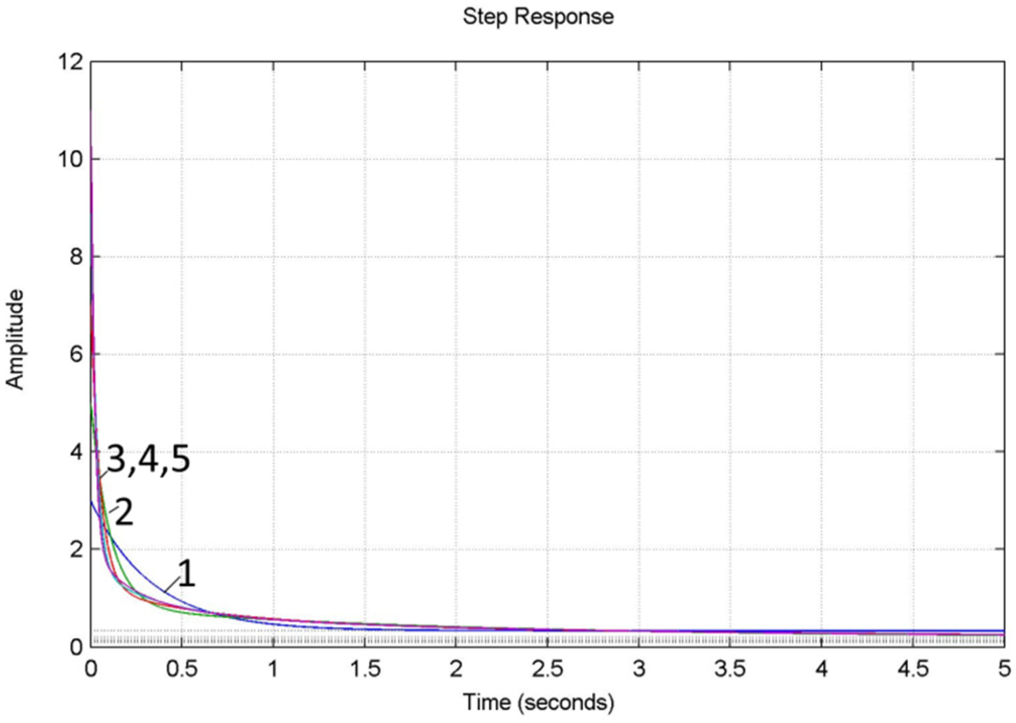
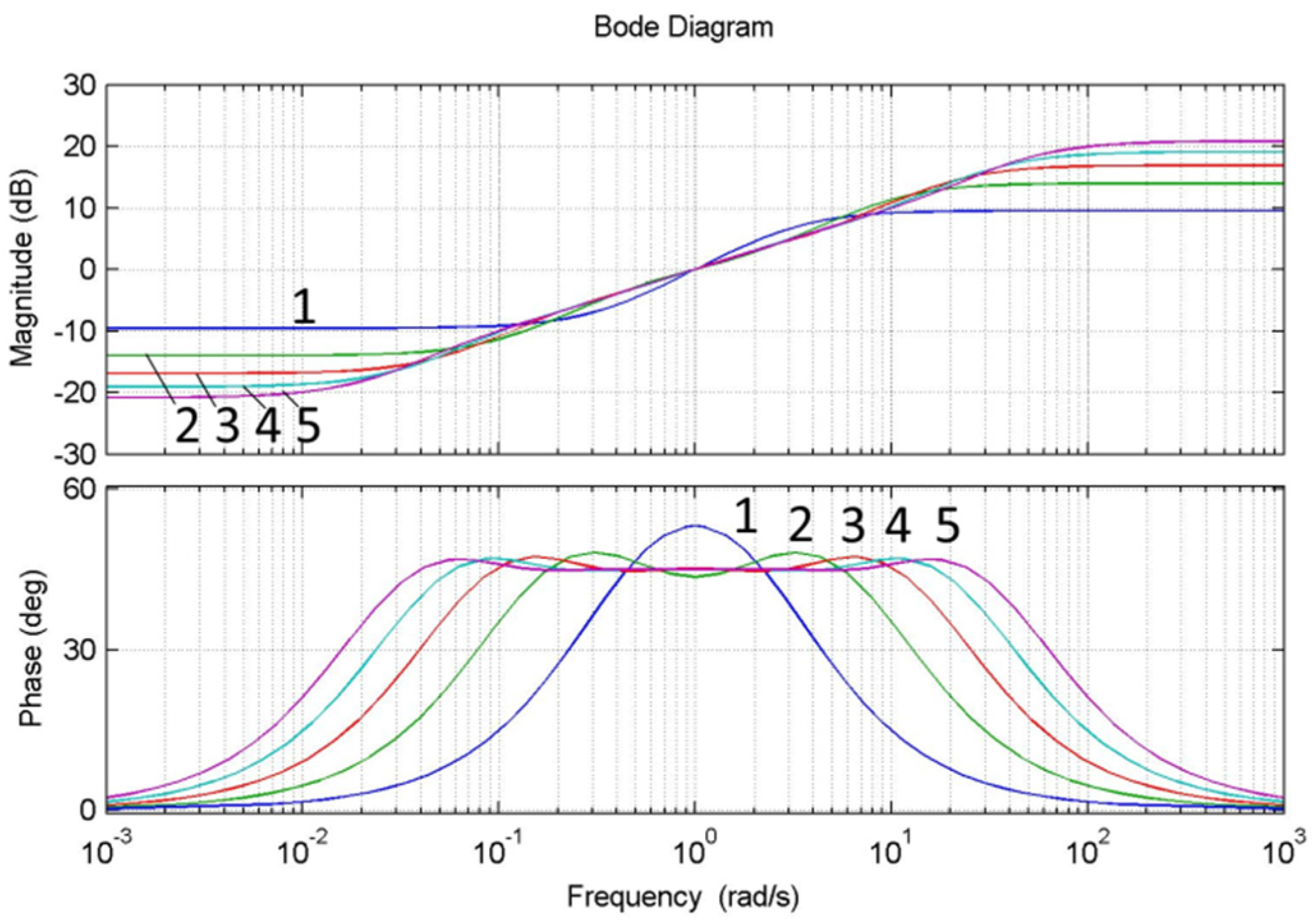
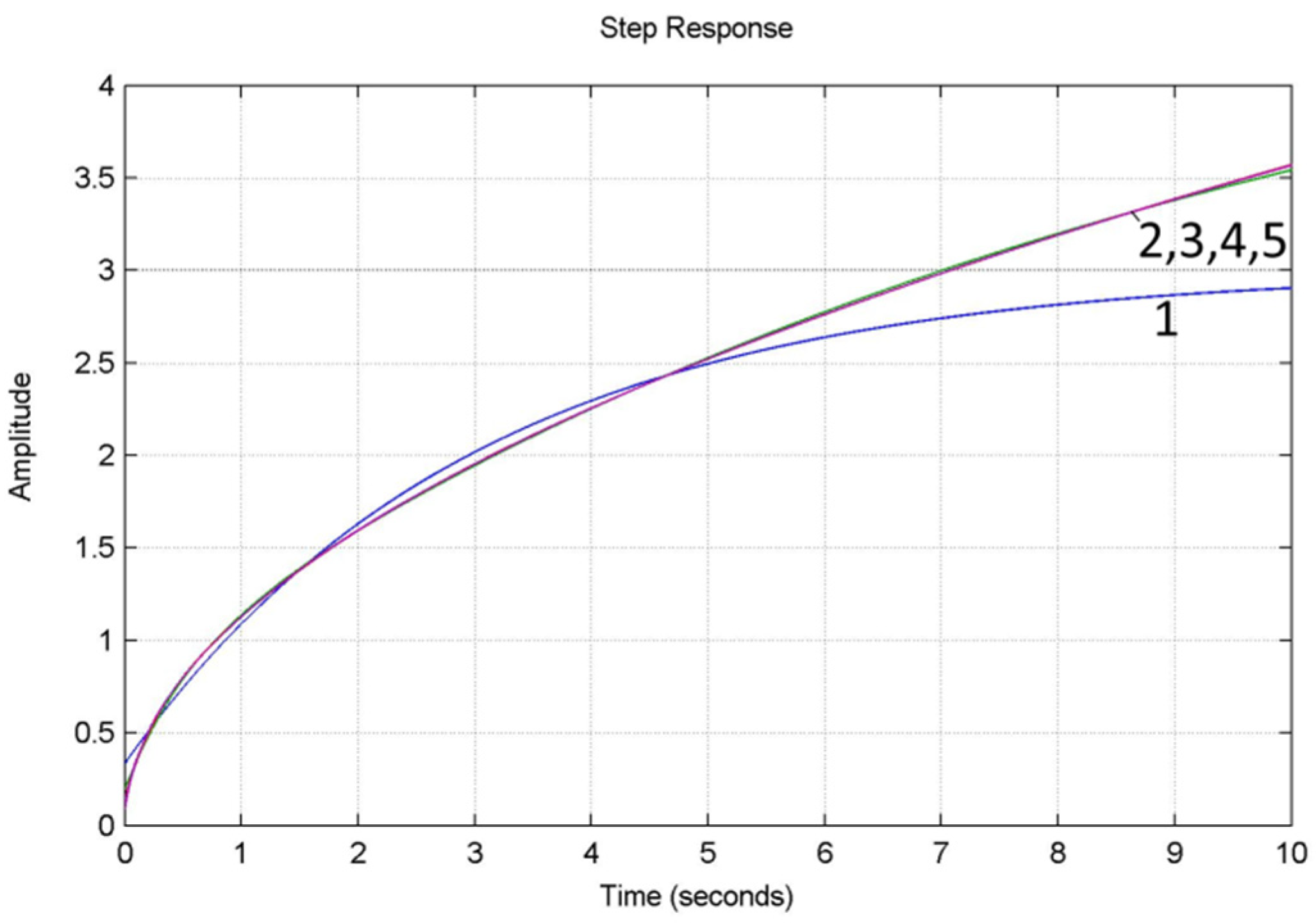
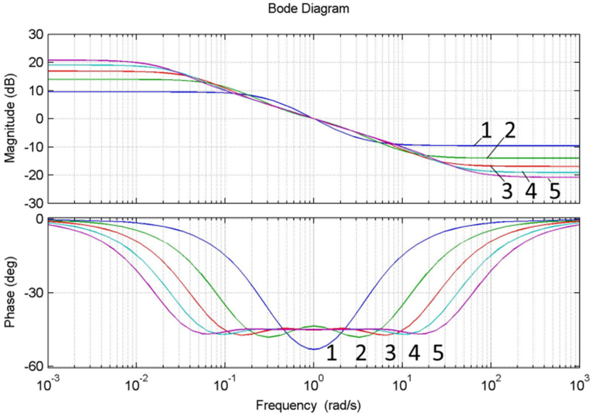
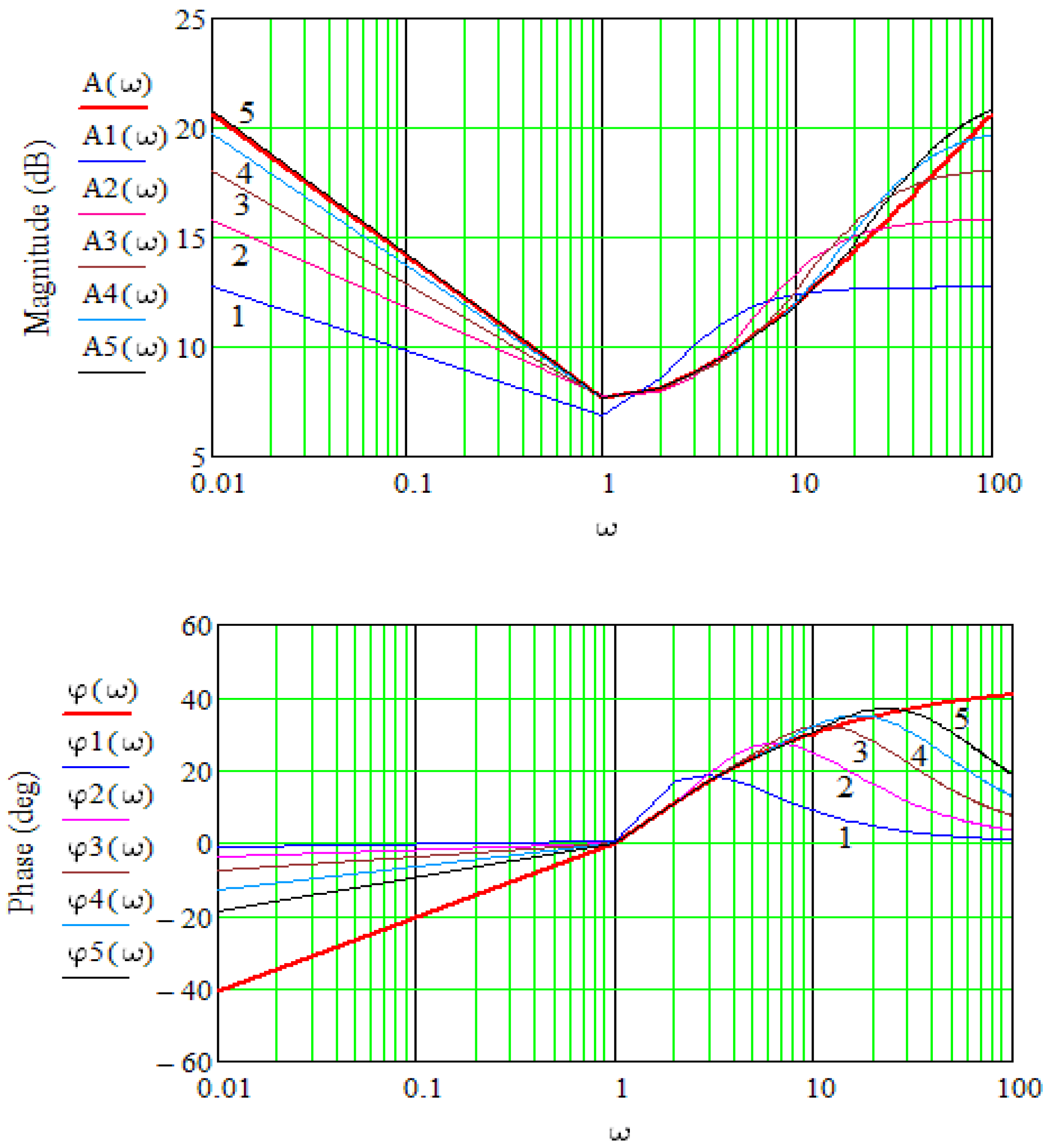
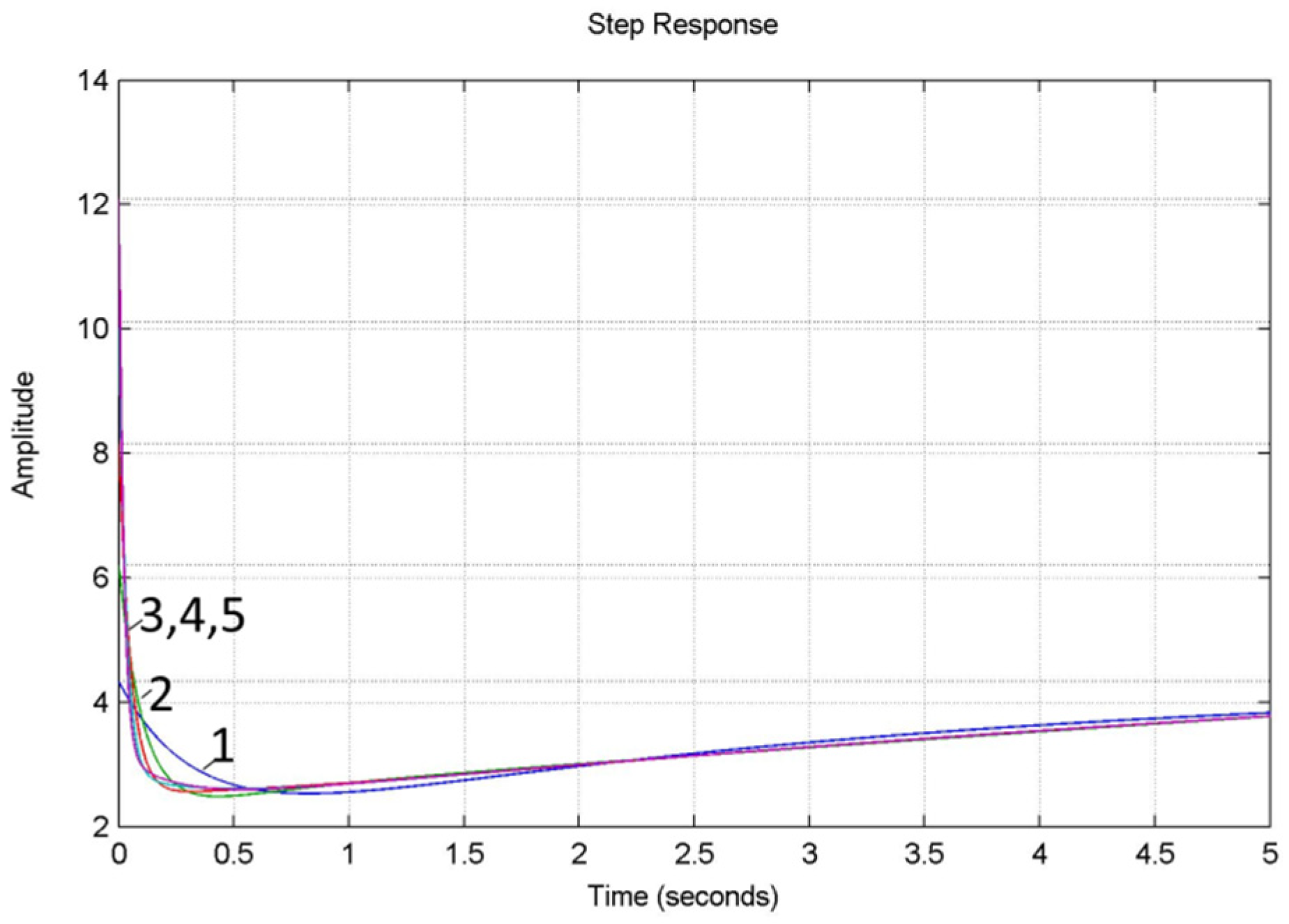
to analyze the accuracy of the approximation of fractional order PI^λD^μ-controller TFs by the method of chain fractions by analyzing the transition functions and frequency characteristics of the units D^μ(α = μ = 0.5) and I^λ (α = λ = −0.5) for five different orders of decomposition by the method of chain fractions;

-

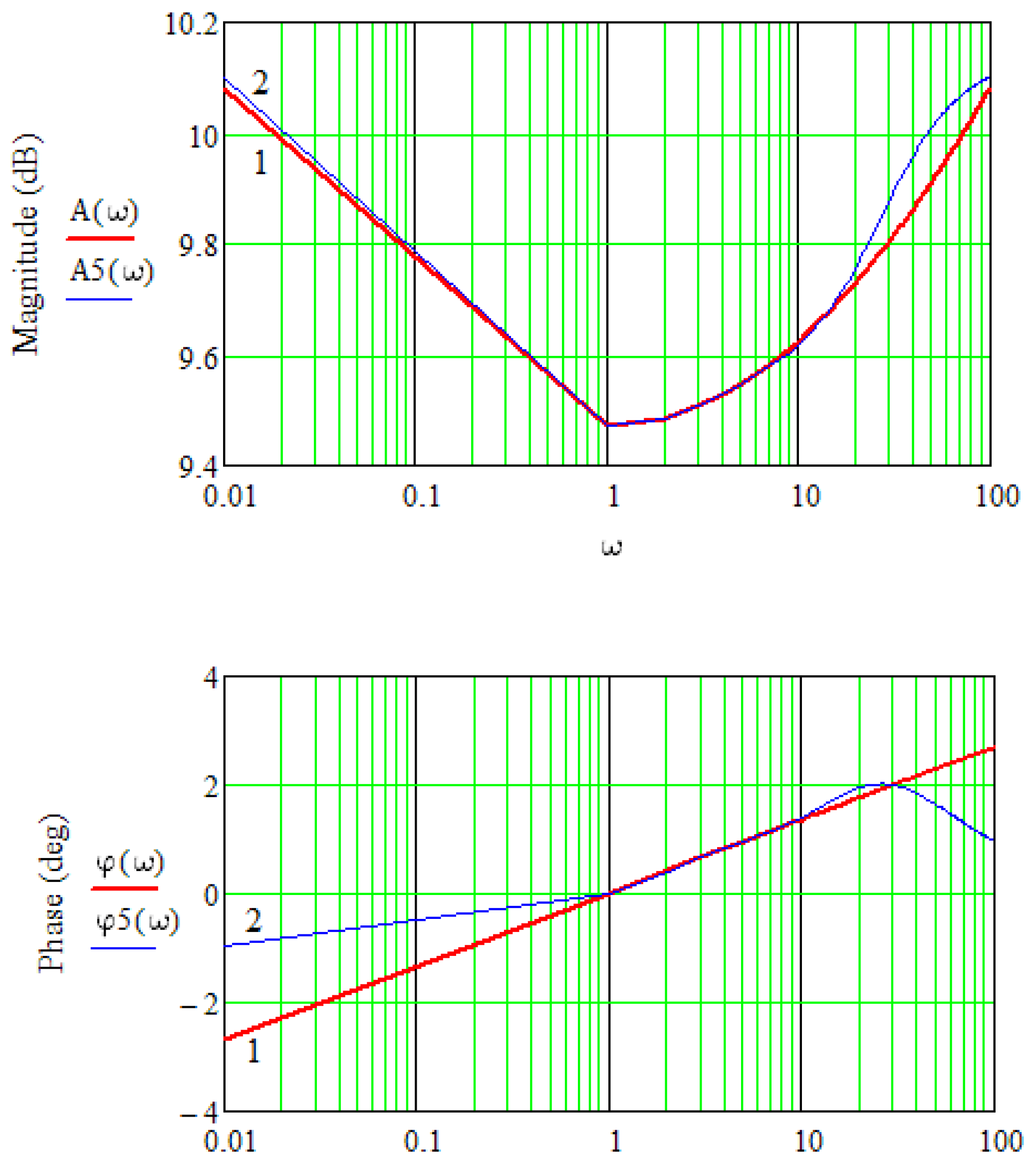
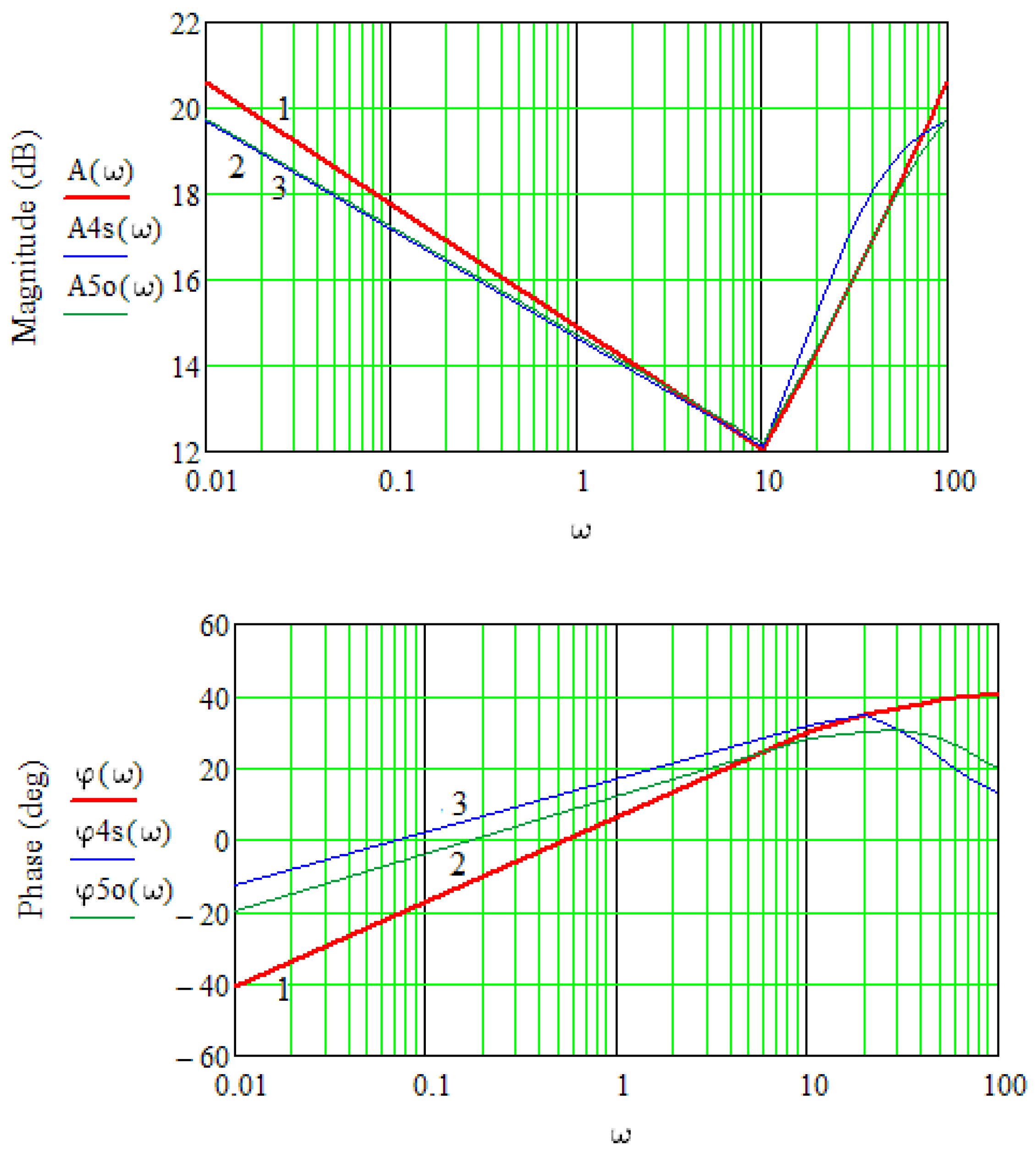
to compare the approximated TFs with polynomials of the same order obtained by the methods of Oustaloup and chain fractions for α = ±0.5 and to establish the advantages of using the method of chain fractions to approximate the TFs of the PI^λD^μ-controllers.

2. Application of the Oustaloup Transformation for Approximations of Fractional Order TFs

The Oustaloup transformation provides an approximation of the fractional order operator $s^{\pm \alpha }$ using transfer functions of the integer order in a given frequency range [${\omega }_l,{\omega }_h$], where there is a lower and upper limit of the frequency range, respectively.

$$s^{\alpha }={\left(\frac{{\omega }_u}{{\omega }_h}\right)}^{\alpha }{\displaystyle \prod }_{k=-N}^{k=N}\frac{1+s/{{\omega }^{\prime }}_k}{1+s/{\omega }_k},$$

(2)

where ${\omega }_u=\sqrt{{\omega }_l{\omega }_h}$, N is the approximation order and ${{\omega }^{\prime }}_k$, ${\omega }_k$ are the zeros and poles of the equivalent integer order TFs, respectively.

The calculation of the zeros and poles of the integer order approximating the TFs is made in accordance with the following expressions:

$${{\omega }^{\prime }}_k={\omega }_l{\left(\frac{{\omega }_h}{{\omega }_l}\right)}^{\left(k+N+0.5-0.5\cdot \alpha \right)/\left(2N+1\right)}$$

(3)

$${\omega }_k={\omega }_l{\left(\frac{{\omega }_h}{{\omega }_l}\right)}^{\left(k+N+0.5+0.5\cdot \alpha \right)/\left(2N+1\right)}$$

(4)

The coefficient of the integer 2N + 1 order approximating the TFs is as follows:

$$k_{\prod }={\left(\frac{{\omega }_u}{{\omega }_h}\right)}^{\alpha },$$

and its orderin approximating the TFs is n = 2N + 1.

Approximating TFs can be written as the ratio of n-order polynomials as follows:

$$W\left(s\right)=k_{\prod }\frac{b_n{s}^n+b_{n-1}{s}^{n-1}+\dots +b_{1}s+b_0}{a_n{s}^n+a_{n-1}{s}^{n-1}+\dots +a_{1}s+a_0}=\frac{P\left(s\right)}{Q\left(s\right)}.$$

(5)

Below, there are exemplified appropriate integer order transfer function expressions obtained by applying the Oustaloup transformation (2) with n = 1, 2 with regard to fractional order differential and integral units, which are adjusted to the following form (5):

(1)

integral fractional unit $W\left(s\right)=s^{-0.5}$

N = 1

$$s^{-0.5}=\frac{0.1s^3+4.867s^2+10.49s+1}{s^3+10.49s^2+4.867s+0.1};$$

(6)

N = 2

$$s^{-0.5}=\frac{0.1s^5+7.497s^4+76.85s^3+121.8s^2+29.85s+1}{s^5+29.85s^4+121.8s^3+76.85s^2+7.497s+0.1};$$

(7)

(2)

differential fractional unit $W\left(s\right)=s^{0.5}$

N = 1

$$s^{0.5}=\frac{10s^3+104.9s^2+48.67s+1}{s^3+48.67s^2+104.9s+10};$$

(8)

N = 2

$$s^{0.5}=\frac{10s^5+298.5s^4+1218s^3+768.5s^2+74.97s+1}{s^5+74.97s^4+768.5s^3+1218s^2+298.5s+10}$$

(9)

3. Application of Chain Fractions for Approximation ofthe Fractional Order Operator $s^{\mp \alpha }$

Let us consider the possibility of applying the theory of chain fractions [5,6,7,8,9] to the approximate $s^{\pm \alpha }$ TF components of PI^λD^μ-controllers and their subsequent technical implementation. According to this theory [5,10,11,12,13,14], any power function can be extended to a chain fraction. In this case, for a binomial of arbitrary degree α, where the Laplace operator does not yet act as a variable, we can write the following expression:

$${\left(1+x\right)}^{\alpha }=\frac{1}{1-}\frac{x\alpha }{1+}\frac{\left(1+\alpha \right)x}{2+}\frac{\left(1-\alpha \right)x}{3+}\frac{\left(2+\alpha \right)x}{2+}\frac{\left(2-\alpha \right)x}{5+---}.$$

(10)

For simplicity of the analysis, we limit ourselves to the number of elements of the chain fraction in order to obtain the highest order of the approximated TF polynomials equal to one. Then, we obtain the following:

$${\left(1+x\right)}^{\alpha }=\frac{1}{1-\alpha \cdot \frac{x}{1+\left(1+\alpha \right)\cdot \frac{x}{2}}}=\frac{x+\alpha \cdot x+2}{x-\alpha \cdot x+2}.$$

(11)

Let us replace the above-mentioned Expression (11) by using the Laplace operator as a variable $x=s-1$ as follows:

$${\left(s\right)}^{\alpha }=\frac{s-\alpha +\alpha \cdot s+1}{s+\alpha -\alpha \cdot s+1}$$

Thus, if α = 0.5, we obtain the following:

$${\left(s\right)}^{0.5}=\frac{3s+1}{s+3}.$$

(12)

Accordingly, if α = −0.5, we obtain the following:

$${\left(s\right)}^{-0.5}=\frac{s+3}{3s+1}.$$

(13)

The obtained results are much simpler than the results obtained on the basis of the Oustaloup transformation.

For higher orders of TFs from n = 2 to n = 5, under the condition that 0 < α < 1, we obtain the following:

If n = 2, we obtain the following:

$$\begin{array}{l}{\left(1+x\right)}^{\alpha }=\frac{1}{1-\alpha \cdot \frac{x}{1+\left(1+\alpha \right)\cdot \frac{x}{2+\left(1-\alpha \right)\frac{x}{3+\left(2+\alpha \right)\cdot \frac{x}{2}}}}}=\\ =\frac{{\alpha }^2{x}^2+3\alpha x^2+6\alpha x+2x^2+12x+12}{{\alpha }^2{x}^2-3\alpha x^2-6\alpha x+2x^2+12x+12}.\end{array}$$

(14)

Having replaced $x=s-1$, Expression (14) looks as follows:

$${\left(s\right)}^{\alpha }=\frac{{\alpha }^2{s}^2+3\alpha s^2+2s^2-2{\alpha }^{2}s+8s+{\alpha }^2-3\alpha +2}{{\alpha }^2{s}^2-3\alpha s^2+2s^2-2{\alpha }^{2}s+8s+{\alpha }^2+3\alpha +2}.$$

Thus, if α = 0.5, we obtain the following: it is corect

$${\left(s\right)}^{0.5}=\frac{5s^2+10s+1}{s^2+10s+5}.$$

(15)

Accordingly, if α = −0.5, we obtain the following:

$${\left(s\right)}^{-0.5}=\frac{s^2+10s+5}{5s^2+10s+1}.$$

(16)

The obtained results are simpler than the results obtained on the basis of the Oustaloup transformation (n = 1).

In the same way, TFs from n = 3 to n = 5 are calculated as follows. If n = 3, we obtain the following:

$$\begin{array}{c}{\left(1+x\right)}^{\alpha }=\frac{1}{1-\alpha \cdot \frac{x}{1+\left(1+\alpha \right)\cdot \frac{x}{2+\left(1-\alpha \right)\frac{x}{3+\left(2+\alpha \right)\cdot \frac{x}{2+\left(2-\alpha \right)\cdot \frac{x}{5+\left(3+\alpha \right)\cdot \frac{x}{2}}}}}}}\\ =\frac{{\alpha }^3{x}^3+6{\alpha }^2{x}^3+12{\alpha }^2{x}^2+11\alpha x^3+60\alpha x^2+60\alpha x+}{{\alpha }^3{x}^3-6{\alpha }^2{x}^3-12{\alpha }^2{x}^2+11\alpha x^3+60\alpha x^2+60\alpha x-}\frac{6x^3+72x^2+180x+120}{6x^3-72x^2-180x-120}.\end{array}$$

(17)

Having replaced $x=s-1$, Expression (17) looks as follows:

$$\begin{array}{c}{\left(s\right)}^{\alpha }=\frac{{\alpha }^3{s}^3+6{\alpha }^2{s}^3+11a{s}^3+6s^3-3{\alpha }^3{s}^2-6{\alpha }^2{s}^2+27\alpha s^2+}{6{\alpha }^2{s}^3-{\alpha }^3{s}^3-11a{s}^3+6s^3+3{\alpha }^3{s}^2-6{\alpha }^2{s}^2-27\alpha s^2+}\\ \frac{+54s^2+3{\alpha }^{3}s-6{\alpha }^{2}s-27\alpha s+54s-{\alpha }^3+6{\alpha }^2-11\alpha +6}{+54s^2-3{\alpha }^{3}s-6{\alpha }^{2}s+27\alpha s+54s+{\alpha }^3+6{\alpha }^2+11\alpha +6},\end{array}$$

If n = 4, we obtain the following:

$$\begin{array}{l}{\left(1+x\right)}^{\alpha }=\\ \hspace{1em}\hspace{1em}\hspace{1em}=\frac{1}{1-\alpha \cdot \frac{x}{1+\left(1+\alpha \right)\cdot \frac{x}{2+\left(1-\alpha \right)\frac{x}{3+\left(2+\alpha \right)\cdot \frac{x}{2+\left(2-\alpha \right)\cdot \frac{x}{5+\left(3+\alpha \right)\cdot \frac{x}{2+\left(3-\alpha \right)\cdot \frac{x}{7+\left(4+\alpha \right)\cdot \frac{x}{2}}}}}}}}}=\\ =\frac{{\alpha }^4{x}^4+10{\alpha }^3{x}^4+20{\alpha }^3{x}^3+35{\alpha }^2{x}^4+180{\alpha }^2{x}^3+}{{\alpha }^4{x}^4-10{\alpha }^3{x}^4-20{\alpha }^3{x}^3+35{\alpha }^2{x}^4+180{\alpha }^2{x}^3+}\\ \frac{+180{\alpha }^2{x}^2+50\alpha x^4+520\alpha x^3+1260\alpha x^2+840\alpha x+24x^4+}{+180{\alpha }^2{x}^2-50\alpha x^4-520\alpha x^3-1260\alpha x^2-840\alpha x+24x^4+}\\ \frac{+480x^3+2160x^2+3360x+1680}{+480x^3+2160x^2+3360x+1680}\end{array}$$

(18)

Having replaced $x=s-1$, Expression (18) looks as follows:

$$\begin{array}{l}{\left(s\right)}^{\alpha }\\ =\frac{{\alpha }^4{s}^4+10{\alpha }^3{s}^4+35{\alpha }^2{s}^4+50\mathsf{\alpha }{s}^4+24s^4-4{\alpha }^4{s}^3-20{\alpha }^3{s}^3+40{\alpha }^2{s}^3+}{{\alpha }^4{s}^4-10{\alpha }^3{s}^4+35{\alpha }^2{s}^4-50\mathsf{\alpha }{s}^4+24s^4-4{\alpha }^4{s}^3+20{\alpha }^3{s}^3+40{\alpha }^2{s}^3-}\\ \frac{+320\alpha s^3+384s^3+6{\alpha }^4{s}^2-150{\alpha }^2{s}^2+864s^2-4{\alpha }^{4}s+20{\alpha }^{3}s+40{\alpha }^{2}s-}{-320\alpha s^3+384s^3+6{\alpha }^4{s}^2-150{\alpha }^2{s}^2+864s^2-4{\alpha }^{4}s-20{\alpha }^{3}s+40{\alpha }^{2}s+}\\ \hspace{1em}\frac{-320\alpha s+384s+{\alpha }^4-10{\alpha }^3+35{\alpha }^2-50\alpha +24}{+320\alpha s+384s+{\alpha }^4+10{\alpha }^3+35{\alpha }^2+50\alpha +24}\end{array}$$

If n = 5, we obtain the following:

$$\begin{array}{l}\hspace{1em}\hspace{1em}\hspace{1em}\hspace{1em}\hspace{1em}\hspace{1em}\hspace{1em}\hspace{1em}\hspace{1em}{\left(1+x\right)}^{\alpha }=\\ =\frac{1}{1-\alpha \cdot \frac{x}{1+\left(1+\alpha \right)\cdot \frac{x}{2+\left(1-\alpha \right)\frac{x}{3+\left(2+\alpha \right)\cdot \frac{x}{2+\left(2-\alpha \right)\cdot \frac{x}{5+\left(3+\alpha \right)\cdot \frac{x}{2+\left(3-\alpha \right)\cdot \frac{x}{7+\left(4+\alpha \right)\cdot \frac{x}{2+\left(4-\alpha \right)\cdot \frac{x}{9+\left(5+\alpha \right)\cdot \frac{x}{2}}}}}}}}}}}\\ =\frac{{\alpha }^5{x}^5+15{\alpha }^4{x}^5+30{\alpha }^4{x}^4+85{\alpha }^3{x}^5+420{\alpha }^3{x}^4+}{{\alpha }^5{x}^5-15{\alpha }^4{x}^5-30{\alpha }^4{x}^4+85{\alpha }^3{x}^5+420{\alpha }^3{x}^4+}\\ \frac{+420{\alpha }^3{x}^3+225{\alpha }^2{x}^5+2130{\alpha }^2{x}^4+5040{\alpha }^2{x}^3+3360{\alpha }^2{x}^2+}{+420{\alpha }^3{x}^3-225{\alpha }^2{x}^5-2130{\alpha }^2{x}^4-5040{\alpha }^2{x}^3-3360{\alpha }^2{x}^2+}\\ \frac{+274\alpha x^5+4620{\alpha }^1{x}^4+19740{\alpha }^1{x}^3+30240{\alpha }^1{x}^2+15120{\alpha }^1{x}^1+}{+274\alpha x^5+4620{\alpha }^1{x}^4+19740{\alpha }^1{x}^3+30240{\alpha }^1{x}^2+15120{\alpha }^1{x}^1-}\\ \frac{+120x^5+3600x^4+25200x^3+67200x^2+75600x^1+30240}{-120x^5-3600x^4-25200x^3-67200x^2-75600x^1-30240}\end{array}$$

(19)

Having replaced $x=s-1$, Expression (19) looks as follows:

$$\begin{array}{c}{\left(s\right)}^{\alpha }=\frac{{\alpha }^5{s}^5+15{\alpha }^4{s}^5+85{\alpha }^3{s}^5+225{\alpha }^2{s}^5+274\alpha s^5+120s^5-5{\alpha }^5{s}^4-}{15{\alpha }^4{s}^5-{\alpha }^5{s}^5-85{\alpha }^3{s}^5+225{\alpha }^2{s}^5-274\alpha s^5+120s^5+5{\alpha }^5{s}^4-}\\ \frac{-45{\alpha }^4{s}^4-5{\alpha }^3{s}^4+1005{\alpha }^2{s}^4+3250\alpha s^4+3000s^4+10{\alpha }^5{s}^3+30{\alpha }^4{s}^3-}{-45{\alpha }^4{s}^4+5{\alpha }^3{s}^4+1005{\alpha }^2{s}^4-3250\alpha s^4+3000s^4-10{\alpha }^5{s}^3+30{\alpha }^4{s}^3+}\\ \frac{-410{\alpha }^3{s}^3-1230{\alpha }^2{s}^3+4000\alpha s^3+12000s^3-10{\alpha }^5{s}^2+30{\alpha }^4{s}^2+410{\alpha }^3{s}^2-}{+410{\alpha }^3{s}^3-1230{\alpha }^2{s}^3-4000\alpha s^3+12000s^3+10{\alpha }^5{s}^2+30{\alpha }^4{s}^2-410{\alpha }^3{s}^2-}\\ \frac{-1230{\alpha }^2{s}^2-4000{\alpha }^1{s}^2+12000s^2+5{\alpha }^5{s}^1-45{\alpha }^4{s}^1+5{\alpha }^3{s}^1+1005{\alpha }^2{s}^1-}{-1230{\alpha }^2{s}^2+4000{\alpha }^1{s}^2+12000s^2-5{\alpha }^5{s}^1-45{\alpha }^4{s}^1-5{\alpha }^3{s}^1+1005{\alpha }^2{s}^1+}\\ \frac{-3250{\alpha }^1{s}^1+3000s^1-s^5+15s^4-85s^3+225s^2-274s+120}{+3250{\alpha }^1{s}^1+3000s^1+s^5+15s^4+85s^3+225s^2+274s+120}\end{array}$$

So, for example, if $\alpha =0.5$ we obtain the following:

n = 3:

$${\left(s\right)}^{0.5}=\frac{7s^3+35s^2+21s+1}{s^3+21s^2+35s+7};$$

(20)

n = 4:

$${\left(s\right)}^{0.5}=\frac{9s^4+84s^3+126s^2+36s+1}{s^4+36s^3+126s^2+84s+9};$$

(21)

n = 5:

$${\left(s\right)}^{0.5}=\frac{11s^5+165s^4+462s^3+330s^2+55s+1}{s^5+55s^4+330s^3+462s^2+165s+11}.$$

(22)

Accordingly, if $\alpha =-0.5$, we obtain the following:

n = 3:

$${\left(s\right)}^{-0.5}=\frac{s^3+21s^2+35s+7}{7s^3+35s^2+21s+1};$$

(23)

n = 4:

$${\left(s\right)}^{-0.5}=\frac{s^4+36s^3+126s^2+84s+9}{9s^4+84s^3+126s^2+36s+1};$$

(24)

n = 5:

$${\left(s\right)}^{-0.5}=\frac{s^5+55s^4+330s^3+462s^2+165s+11}{11s^5+165s^4+462s^3+330s^2+55s+1}.$$

(25)

Figure 1 shows the graphs of the transition functions of theD^μ parts (α = μ = 0.5), which are described by the TFs (12), (15), (20)–(22). Figure 2 demonstrates the frequency characteristics (Bode diagrams) of these TFs.

Similarly, the graphs of the transition functions of theI^λ parts (α = λ = −0.5), which are described by the TFs (13), (16), (23)–(25) (Figure 3), and the frequency characteristics of these TFs (Figure 4) were obtained.

Using the approximations of theI^λ and D^μ parts, as components of the fractional order controllers, we will approximate the PI^λD^μ-controllers with different λ and μ values of their TFs. For example, if α = ±0.5, then (1) turns into the following:

$$W\left(\omega \right)=1+\frac{1}{{\left(j\omega \right)}^{0.5}}+{\left(j\omega \right)}^{0.5}$$

(26)

For five different decomposition orders of the PI^λD^μ-controller (26), the frequency characteristics of such controller were obtained by the method of chain fractions (Figure 5). Here are the corresponding frequency characteristics (red graphs), which are calculated for the fractional TFs using the Mathcad application package. We consider these graphs as reference.

It follows from the obtained graphs that the position of the frequency characteristics in relation to the reference characteristics for frequencies at most 1rad/s significantly depends on the order of approximations. The difference between the frequency and the reference characteristics starts to considerably decrease from the fifth order of approximation. Thus, in this case, the standard deviation σ for the amplitude–frequency characteristic is σ₁ = 0.0596 and for the phase–frequency characteristic is σ₂ = 6.316.

If the frequency exceeds 1 rad/s, then for each order of approximation there is a frequency range, for which the lowest value of σ is provided. Thus, if n = 1, then the smallest value σ₁ = 1087 for the amplitude–frequency characteristic remains in the frequency range between 1rad/s and 10rad/s. With respect to the phase–frequency characteristics, the lowest value σ₂ = 3.85 remains in the frequency range between 1 rad/s and 4 rad/s. If we apply the approximation order n = 5, then the same values of σ can be provided in the frequency range between 1 rad/s and 100 rad/s for the amplitude–frequency characteristic and between 1 and 40 rad/s for the phase–frequency characteristic.

Therefore, it is recommended to choose the order of approximation based on the analysis of the development of the expected frequency effects of the system.

For clarity of the controller operation, Figure 6 shows its transition processes for the part described by Expression (26).

Due to the greater informativeness of the frequency characteristics, we will further analyze these characteristics.

Similarly to the case of α = ±0.5, the frequency characteristics for the TF were obtained when α = ± 0.1, as follows:

$$W\left(\omega \right)=1+\frac{1}{{\left(j\omega \right)}^{0.1}}+{\left(j\omega \right)}^{0.1}.$$

(27)

These graphs are shown in Figure 7. Similarly, the studies were performed to change α in the range from ±0.1 to ±0.9 in various combinations.

For all investigated systems, the same conclusions are made for obtaining the specified accuracy of the frequency characteristics in the appropriate frequency range, as those made for the case of α = ±0.5.

The obtained results showed the possibility of applying the TF approximation of the PI^λD^μ-controller by the method of chain fractions with different values for λ and μ.

In order to compare the methods of Oustaloup and chain fractions, we analyzed the frequency characteristics approximated from the condition n = 5 for the method of Oustaloup and n = 4 for the method of chain fractions if α = ±0.5 is inherent in the TF.

The chain fraction method is as follows:

$$\begin{array}{c}W4cf\left(\omega \right)=1+\frac{{\left(j\omega \right)}^4+36{\left(j\omega \right)}^3+126{\left(j\omega \right)}^2+84\left(j\omega \right)+9}{9{\left(j\omega \right)}^4+84{\left(j\omega \right)}^3+126{\left(j\omega \right)}^2+36\left(j\omega \right)+1}+\\ +\frac{9{\left(j\omega \right)}^4+84{\left(j\omega \right)}^3+126{\left(j\omega \right)}^2+36\left(j\omega \right)+1}{{\left(j\omega \right)}^4+36{\left(j\omega \right)}^3+126{\left(j\omega \right)}^2+84\left(j\omega \right)+9}.\end{array}$$

The Oustaloup method is as follows:

$$\begin{array}{l}W5o\left(\omega \right)\\ =1+\frac{0.1{\left(j\omega \right)}^5+7.497{\left(j\omega \right)}^4+76.85{\left(j\omega \right)}^3+121.8{\left(j\omega \right)}^2+29.85\left(j\omega \right)+1}{1{\left(j\omega \right)}^5+29.85{\left(j\omega \right)}^4+121.8{\left(j\omega \right)}^3+76.85{\left(j\omega \right)}^2+7.497\left(j\omega \right)+0.1}+\end{array}$$

$$\hspace{1em}\hspace{1em}+\frac{10{\left(j\omega \right)}^5+298.5{\left(j\omega \right)}^4+1218{\left(j\omega \right)}^3+768.5{\left(j\omega \right)}^2+74.97\left(j\omega \right)+1}{{\left(j\omega \right)}^5+74.97{\left(j\omega \right)}^4+768.5{\left(j\omega \right)}^3+1218{\left(j\omega \right)}^2+298.5\left(j\omega \right)+10}.$$

The frequency characteristics for these two cases are shown in Figure 8.

It follows from the obtained graphs that σ₁ ≈ 9.09, σ₂ = 14.13 in almost the whole investigated frequency range for the method of chain fractions and that σ₁ ≈ 9.42, σ₂ = 14.31 in this frequency range for the Oustaloup method.

The analysis of the obtained results showed almost the same accuracy of approximation of the TF PI^λD^μ-controllers by both methods. It should be noted that this result is achieved by the method of chain fractions of the lower order than the order of the Oustaloup method. This simplifies the implementation of the PI^λD^μ-controller.

4. Conclusions

• Analytical expressions based on the application of the chain fraction theory to approximate the components of the transfer functions of PI^λD^μ-controllers $s^{\pm \alpha }$ have been obtained.
• The accuracy of the approximation of the fractional transfer function by the method of chain fractions has been researched by analyzing the transition functions and frequency characteristics of the units D^μ and I^λ for five different orders of decomposition by the method of chain fractions.
• The comparison of the transfer functions, approximated by different order polynomials, has been conducted. As a result, the possibility of obtaining the same approximation accuracy has been established under the condition of using the method of chain fractions of the lower order. Using this approximation method simplifies the implementation of PI^λD^μ.
• The analysis proved the possibility of using the method of chain fractions to approximate the transfer function of PI^λD^μ-controllers. The accuracy of the same order transfer function approximation is higher when the method of chain fractions is used. Based on the analysis of the system’s performance of the expected frequency effects, it is necessary to choose the appropriate approximation order to ensure the specified accuracy of the approximation.

References

1. Kopchak, B.; Marushchak, Y.; Kushnir, A. Devising a procedure for the synthesis of electromechanical systems with cascade-enabled fractional-order controllers and their study. East.-Eur. J. Enterp. Technol. Inf. Technol. Ind. Control. Syst. 2019, 5, 65–71. [Google Scholar] [CrossRef] [Green Version]
2. Lozynskyy, O.; Mazur, D.; Marushchak, Y.; Kwiatkowski, B.; Lozynskyy, A.; Kwater, T.; Kopchak, B.; Hawro, P.; Kasha, L.; Pękala, R.; et al. Formation of characteristic polynomials on the basis of fractional powers j of dynamic systems and stability problems of such systems. Energies 2021, 14, 7374. [Google Scholar] [CrossRef]
3. Oustaloup, A.; Levron, F.; Nanot, F.; Mathieu, B. Frequency band complex non-integer differentiator: Characterization and synthesis. IEEE Trans. Circuits Syst. I Fundam. Theory Appl. 2000, 47, 25–40. [Google Scholar] [CrossRef]
4. Kopchak, B. Development of fractional order differential-integral controller by using Oustaloup transformation. In Proceedings of the 2016 XII International Conference on Perspective Technologies and Methods in MEMS Design (MEMSTECH), Lviv, Ukraine, 20–24 April 2016; pp. 62–65. [Google Scholar] [CrossRef]
5. Khovanskii, A.N. The Application of Continued Fractions and Their Generalizations to Problems in Approximation Theory; P. Noordhoff: Groningen, The Netherlands, 1963. [Google Scholar]
6. Krishna, B.T.; Reddy, K.V.V.S. Active and passive realization of fractance device of order ½. Act. Passiv. Electron. Compon. 2008, 2008, 369421. [Google Scholar] [CrossRef] [Green Version]
7. Kumar, R.; Perumalla, S.; Vista, J.; Ranjan, A. Realization of single and double cole tissue models using higher order approximation. In Proceedings of the 1st International Conference on Electronics, Materials Engineering and Nano-Technology (IEMENTech), Science City, Kolkata, India, 28–29 April 2017; pp. 1–4. [Google Scholar]
8. Pu, Y.; Yuan, X.; Liao, K. Structuring analog fractance circuit for 1/2 order fractional calculus. In Proceedings of the 6th International Conference on ASIC (ASICON’05), Shanghai, China, 24–27 October 2005; Volume 2, pp. 1136–1139. [Google Scholar]
9. Press, W.H.; Teukolsky, S.A.; Vetterling, W.T.; Flannery, B.P. Section 5.2. Evaluation of Continued Fractions. In Numerical Recipes: The Art of Scientific Computing, 3rd ed.; Cambridge University Press: New York, NY, USA, 2007. [Google Scholar]
10. Cuyt, A.; Brevik Petersen, V.; Verdonk, B.; Waadeland, H.; Jones, W.B. Handbook of Continued Fractions for Special Functions; Springer: Berlin/Heidelberg, Germany, 2008. [Google Scholar]
11. Rockett, A.M.; Szüsz, P. Continued Fractions; World Scientific Press: Singapore, 1992. [Google Scholar]
12. Scheinerman, E.; Pickett, T.; Coleman, A. Another Continued Fraction for π. Am. Math. Mon. 2008, 115, 930–933. [Google Scholar]
13. Collins, D.C. Continued Fractions. MIT Undergrad. J. Math. 1999, 1, 11–20. [Google Scholar]
14. Martin, R.M. Electronic Structure: Basic Theory and Practical Methods; Cambridge University Press: Cambridge, UK, 2004; p. 557. [Google Scholar]
Figure 1. Transition processes of parts (12)—1, (15)—2, (20)—3, (21)—4, (22)—5.
Energies 15 04902 g001
Figure 2. Frequency characteristics of parts (12)—1, (15)—2, (20)—3, (21)—4, (22)—5.
Energies 15 04902 g002
Figure 3. Transition processes of parts (13)—1, (16)—2, (23)—3, (24)—4, (25)—5.
Energies 15 04902 g003
Figure 4. Frequency characteristics of parts (13)—1, (16)—2, (23)—3, (24)—4, (25)—5.
Energies 15 04902 g004
Figure 5. Reference frequency characteristics and frequency characteristics for five approximation orders, if α = ±0.5.
Energies 15 04902 g005
Figure 6. Transition processes of the PIλDμ-controllers (26) for n = 1, 2, …, 5.
Energies 15 04902 g006
Figure 7. Reference frequency characteristics 1 and frequency characteristics for the fifth approximation order if α = ±0.1; 2 for n = 5.
Energies 15 04902 g007
Figure 8. Reference frequency characteristics 1 and frequency characteristics for the TF, approximated by the methods of Oustaloup 2 and chain fractions 3.
Energies 15 04902 g008
Publisher’s Note: MDPI stays neutral with regard to jurisdictional claims in published maps and institutional affiliations.