Article

Application of Selected Machine Learning Techniques for Identification of Basic Classes of Partial Discharges Occurring in Paper-Oil Insulation Measured by Acoustic Emission Technique

1
Institute of Electric Power Engineering and Renewable Energy, Opole University of Technology, 45-758 Opole, Poland
2
Department of Computer Science and Automatics, University of Bielsko-Biala, 43-309 Bielsko-Biala, Poland
3
Walbrzych Special Economic Zone, Invest-Park, 58-306 Walbrzych, Poland
*
Author to whom correspondence should be addressed.
Energies 2022, 15(14), 5013; https://doi.org/10.3390/en15145013
Submission received: 14 May 2022 / Revised: 21 June 2022 / Accepted: 6 July 2022 / Published: 8 July 2022
(This article belongs to the Special Issue Advances in Oil Power Transformers)

Abstract

:
The paper reports the results of a comparative assessment concerned with the effectiveness of identifying the basic forms of partial discharges (PD) measured by the acoustic emission technique (AE), carried out by application of selected machine learning methods. As part of the re-search, the identification involved AE signals registered in laboratory conditions for eight basic classes of PDs that occur in paper-oil insulation systems of high-voltage power equipment. On the basis of acoustic signals emitted by PDs and by application of the frequency descriptor that took the form of a signal power density spectrum (PSD), the assessment involved the possibility of identifying individual types of PD by the analyzed classification algorithms. As part of the research, the results obtained with the use of five independent classification mechanisms were analyzed, namely: k-Nearest Neighbors method (kNN), Naive Bayes Classification, Support Vector Machine (SVM), Random Forests and Probabilistic Neural Network (PNN). The best results were achieved using the SVM classification tuned with polynomial core, which obtained 100% accuracy. Similar results were achieved with the kNN classifier. Random Forests and Naïve Bayes obtained high accuracy over 97%. Throughout the study, identification algorithms with the highest effectiveness in identifying specific forms of PD were established.

1. Introduction

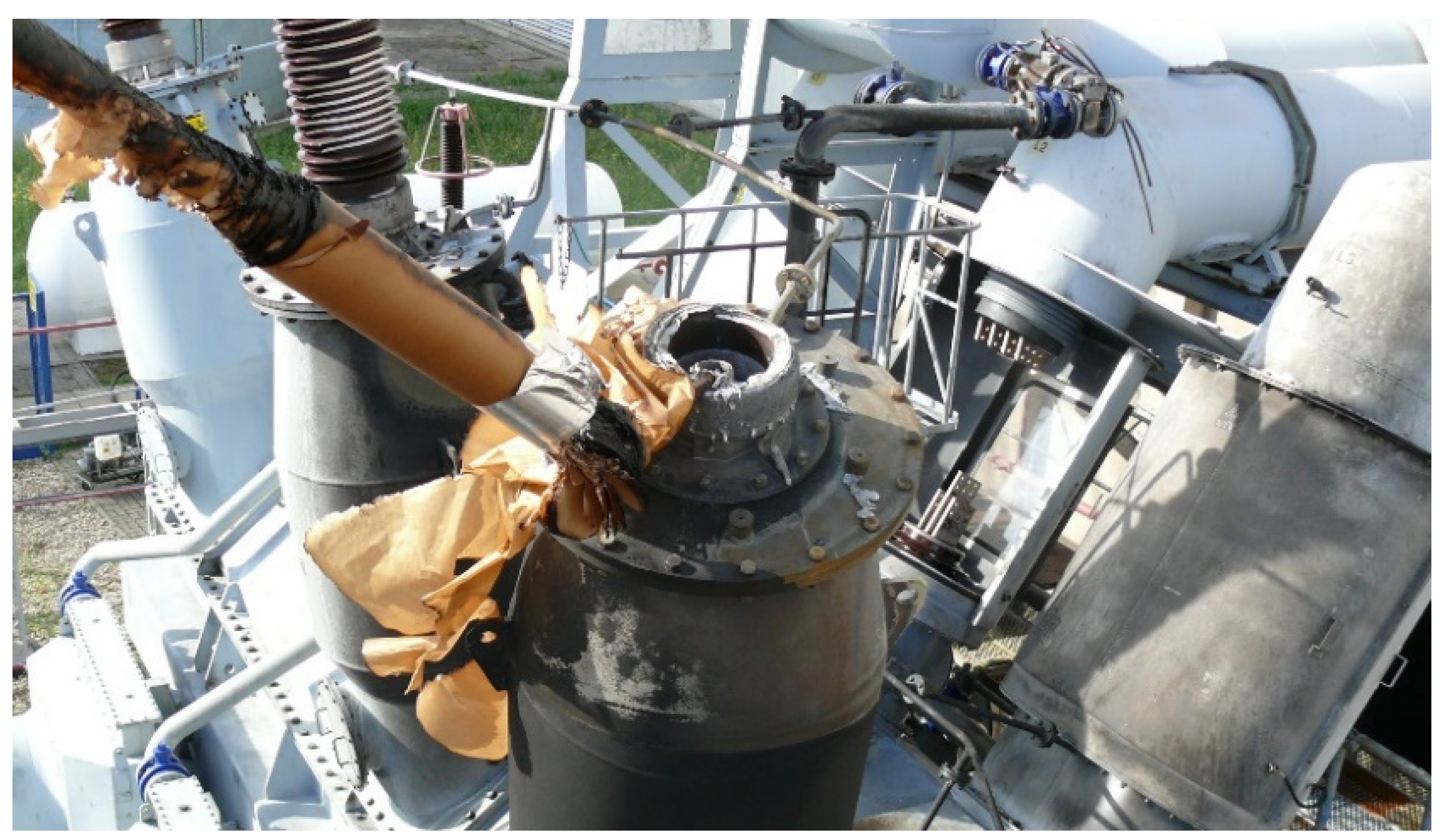
Some of the main causes for the failure of high voltage electrical devices operating in the power system are related to faults that occur in their internal insulation systems. Such faults can be attributed not only to the natural aging processes of the insulation, but also to the occurrence of other phenomena in the transmission and distribution system, including: overvoltages of atmospheric origin, switching overvoltages, dynamic load variations, short circuits accompanied by a high temperature rise as well as considerable electro-dynamic interactions. The local deterioration of the electrical properties of the insulation system, which may be due to the above-mentioned factors, is usually accompanied by partial discharges (PD), whose uncontrolled development leads to complete degradation of the insulation and, consequently, to irreversible fault to a given power facility (Figure 1 and Figure 2).
The elements that assume a critical role for the operation of the power system include power transformers, the investment cost of which is equal to as much as 20% in relation to the total value of all transmission and distribution facilities operated at the power stations. Emergency shutdown of a transformer, most commonly associated with the failure to its insulation system, may lead to significant economic losses, which in extreme conditions may exceed the value of a new transformer by several times. Such expenses result not only from the cost of the potential repair, but also from financial losses due to the failure to supply the contracted volumes of electricity to consumers [1,2,3].
The current state-of-the-art techniques applicable for assessing the technical condition of high-voltage electrical devices increasingly utilize acoustic emission techniques (AE) with the purpose of detecting and measuring the PDs developing inside the insulation system. The main advantage of this method is related to the fact that measurements of parameters characterizing the AE signals generated by PD can be executed directly on power facilities during normal operation. Due to the dynamic development of diagnostic equipment, the main problem with the development of the EA technique is the adequate analysis and interpretation of the resulting data. Correct measurement methodology is not a big threat anymore. The issues discussed in the article concern one of the aspects of the analysis of recorded AE signals, namely the adequate and effective recognition of the so-called patterns of basic forms of PDs.
The AE signals generated by electric discharges can be related to the basic forms of PD [4,5,6] presented in the literature, which in turn are identified with the type of defect and, consequently, with the degree of failure of the paper-oil insulation. The adequately conducted processes of identifying AE signals recorded on the basis of PD can be used as a diagnostic tool. First, the defect of a given insulation system can be identified. Second, it allows for a preliminary assessment of the technical condition of the monitored insulation system of the specific equipment.
PD is defined in the literature [7,8,9] as the current passing through an insulation locally, while its intensity is not sufficient to immediately and directly lose the insulating properties of an insulating material. PD can occur both in a certain area of the insulation system and at a specific point in it. It is worth noting that the occurrence of PD in an insulation system does not result in an immediate breakdown of the insulation. Only its long-term persistence results in a gradual degradation of the system and the formation of a complete discharge that contributes to a loss of insulation properties. For many years, the Department of Electric Power and Renewable Energy at the Opole University of Technology has been conducting scientific research work on the use of the AE method in the diagnostics of insulation systems of high voltage devices. In the course of the conducted scientific research, among others, Own classification of PD includes eight basic classes (also called basic forms of PD), and their classification has been linked to specific types of defects in paper-oil insulation systems:
  • Class 1—partial discharges in the needle–needle system. These discharges may correspond to the PD caused by failure to the insulation of two adjacent turns of the transformer windings.
  • Class 2—partial discharges in the needle–needle system accompanied by freely displaced gas bubbles. Such PD can occur in the oil-paper insulation of the adjacent transformer windings and resulst from the fault or deterioration of the insulation system in oil with high gas mass ratio (due to the developed aging process of dielectrics).
  • Class 3—discharges in the plate–needle system. These discharges may correspond to PD occurring between the faulty part of the transformer winding insulation and grounded flat parts, such as core, yoke, tank or magnetic screens.
  • Class 4—discharges in the surface system of two flat and curved electrodes comprising a paper-oil insulation. PD modeling discharges occurring in the so-called triple point, i.e., at the interface of the live conductors of the transformer winding and the paper dielectric impregnated with electro-insulating oil, one in which the core has a smooth and even surface. This is the most common type of PD.
  • Class 5—discharges in a surface system with one flat electrode, the other multi-needle electrode, between which there is a paper-oil insulation. Discharges that may represent PDs develop at the interface of copper conductors and the paper-oil insulation system (the so-called triple point), in the case where an irregularity occurs in the winding surface (places where a joint occurs between individual winding elements, e.g., in wire splices).
  • Class 6—discharges in the multi-needle–plate in oil system. Discharges that may correspond to PDA occurring between the multi-point insulation failure of the transformer winding and grounded flat parts such as core, yoke, tank or magnetic screens.
  • Class 7—discharges in the multi-needle–plate in oil system with freely displaced gas bubbles. The PD modeling discharges between the fragment of the transformer winding comprises faults as a result of the degradation of the layers of impregnated cable paper (instead of one PD generation point, there may be several or a dozen of them within a small distance), and the grounded elements such as core, yoke, tank or magnetic screens.
  • Class 8—discharges in a multi-needle–plate system with freely displaced solid particles with non-specific potential. Such discharges can represent PDs that occur in transformers with a long service life, during which aging processes of paper insulation take place, combined with the separation of cellulose fibers [4,7,8,10].
A database of AE signals comprising several hundred plots developed in the time domain constitutes the basis for the scientific research carried out in order to verify the suitability of selected machine learning methods for identifying the basic forms of PD, the results of which are presented in this paper. These plots have been identified to fit into the eight classes mentioned above. The EA signals that make up the subject base were generated and recorded in laboratory conditions with the use of systems modeling the basic forms of PD. Detailed characteristics of the generation conditions of individual PD forms and the metrological conditions of measurements of AE signals are presented, among others, in a series of publications [4,7,8,10,11,12].
The issues of scientific research undertaken for this article constitute the focus of research concerned with effective and efficient identification of single-source PD forms that may occur in paper-oil insulation systems of high-voltage devices, e.g., in high-power transformers. Currently, the identification of basic PD forms on the basis of acoustic signals measured with the AE method has been repeatedly performed based on the results of the analysis: frequency, time-frequency and statistical correlations, mainly by means of a comparison of the graphical and numerical representation of selected AE signal descriptors. This resulted in a significantly longer duration of processing time involving the measurement data, and the results obtained on this basis could not be comprehensively interpreted in an absolute manner.
Moreover, the methodology that has been applied to date made it impossible to estimate the effectiveness of identifying each of the measured types of PD. The paper contains a proposition of the use of selected machine learning mechanisms with the purpose of identifying basic forms of PD (named above as classes), which will significantly accelerate the currently utilized computational procedures and can contribute to the improvement in the efficiency of their identification. The application of the proposed signal processing methods will also serve to eliminate the human factor related to the subjective interpretation of the results obtained during the analyses, and, as a consequence, it may significantly unify and efficiently standardize the methodology of assessing the condition of the insulation system. The performed scientific research, the results of which are presented in this article, constitute the next stage of research aimed at designing and implementing a diagnostic system serving for the correct assessment of the insulation condition of power equipment based on on-line measurements of signals generated by PDs using AE.

2. Characteristics of Selected Machine Learning Methods

The article contains a proposition designed to automate the process of identifying basic PD types that may occur in the paper-oil insulation system of power transformers by application of machine learning algorithms (ML). The use of such algorithms offers the possibility of establishing complex relations and finding principles using data mining techniques. Machine learning is derived from statistics, which can also be regarded as the art of extracting knowledge from data. In particular, such methods as linear regression and Bayesian statistics, which have been utilized for over 200 years, are still found in the spotlight nowadays. Machine learning is usually subdivided according to the types of problems that need to be solved. The rough division is as follows:
  • supervised learning
  • unsupervised learning
  • reinforcement learning
In the case of supervised learning [13], a training set with valid target values is provided. In the simplest cases, we have to deal with the closed question with answers in the form of yes/no, and the problem is then called a binary classification. In unsupervised learning [14], there is a tendency to establish relations in some data without knowing their primary (correct) classification. Reinforced learning [15] is commonly applied in situations where an intelligent agent, such as an autonomous car, needs to operate in an environment where feedback regarding the right or wrong alternatives is available with some delay. It is also used in games where the result can only be determined at the end of the game. The most common classification algorithms include: the k-Nearest Neighbors method [16], Naive Bayes Classification [13], Support Vector Machine [17,18], Random Forests [19], Bagging methods [20] as well as various types of neural networks [21,22,23,24,25].
A classifier represents an algorithm applicable for determining the decision class of objects by their values based on attributes in the conditional form. Classifiers can be described by logical formulae, decision trees or mathematical formulae. Many decision problems can be described as a problem of classification. Decision Support System (DSS) is a computer system that provides tools that can be utilized for solving classification problems. The main requirements that are set for this system include: quick decision-making capacity, scalability, efficiency, rationality and the ability to cooperate with an expert (consulting, adaptation and negotiation). Pre-processing is often used to simplify the model and improve its accuracy in order to optimize and reduce the number of input attributes [14]. The common methods applied for measuring associations include the analysis of principal components [26,27,28,29] as well as the analysis of canonical correlations [30,31].
In knowledge engineering, support-vector machines (SVMs) are supervised learning methods with related learning algorithms that resolve data for classification and regression analysis problems. A range of various kernels (HyperTangent, Polynomial and RBF) are supported. The SVM learner supports multiple class problems as well (by computing the hyperplane between each class and the others), but it is worth noting that this will increase the processing time. The SVM learning algorithm used is described by Keerthi et al. [32] and Platt [33]. The k-Nearest Neighbors classifier can be applied to select an adequate value of k based on cross-validation. This algorithm can also use instance-based learning (IBL) that generates classification predictions applying unique instances (distance weighting). This issue was proposed by Aha et al. [34]. The IBL methods could learn any problem that can be described as a finite union of closed hypercurves of finite size in the instance space. Each instance is preferred from any constant and constrained continuous distribution. A probabilistic neural network (PNN) is a feed-forward neural network, which is widely used in pattern recognition and classification problems. The first layer of this neural network calculates the distance from the input vector to the training input vectors, when an input data is entered. This stage creates a vector where its elements indicate the differences between the input and the training input. The next layer totals the weight for each class of inputs, then creates its net output on the form of a vector of probabilities. In the next step, a fully-complete transfer function on the second layer’s output selects the maximum value of these probabilities, and returns a true (positive identification) for that class and a false (negative identification) for non-targeted classes.
The ML algorithms described above find application in independent datasets. In the case under consideration, the measured time series contains the sound pressure values derived from a specific time interval, which is characterized by considerable sequential connections [14,35] and should be considered as a characteristic of time. This task can be performed through sequence classification, which takes into account series of time series [14,36]. There are a lot of machine learning models and algorithms that can accomplish these jobs, for example: the Markov models [37], sliding window methods [38], Kalman filtering [39], conditional random fields [40], recurrent neural networks [41], deep feedforward neural networks [23], Welch method and Maximum Entropy Markov Models [42,43]. The Welch method [44] serves as a tool for the determination of the estimated spectral power density of the signal. This was presented by research [44,45,46]. The main advantage of this method is to minimize the effect of external noise by averaging and smoothing the momentary spectrum. Furthermore, this algorithm can be used to recognize frequencies which may contain convenient information for classification reasons [46]. Therefore, in the proposed model at the pre-processing stage, the Welch method with the described feature discrimination method and varied ML algorithms were used.

3. Methodology

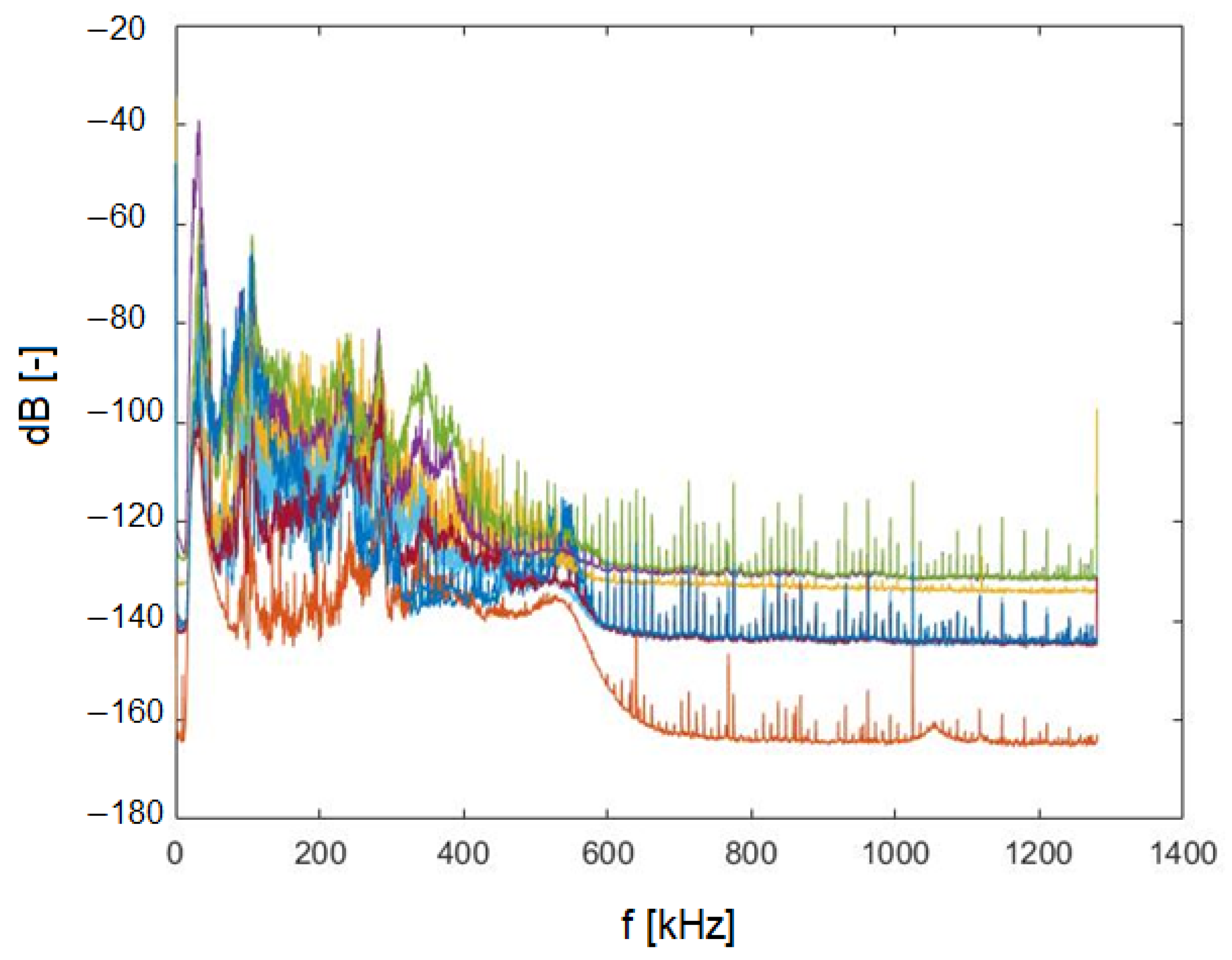
The data that was derived within individual classes were analyzed in the initial phase. Figure 3 shows the frequency analysis graph for all classes using the Welch method [45] with the window width equal to 213. The band of dominant frequencies is in the range of 5–600 kHz, in which characteristic ranges can be distinguished for each of the individual classes. The first is in the 5–100 kHz band, where the spectrum waveform reaches the maximum value for each class. In the 600–1300 kHz frequency range, the spectrum is practically flat; however, there are three local resonant peaks in the range of the following frequencies: 800 kHz, 1000 kHz and 1300 kHz. Due to the use of the preliminary filtering, the transformation results for individual classes are significantly different from each other and can be subjected to subsequent classification.
A preliminary study was carried out to determine the effectiveness of the classification for a given window width on the basis of classifiers with standard parameters [47]. The results of the analysis are summarized in Table 1.
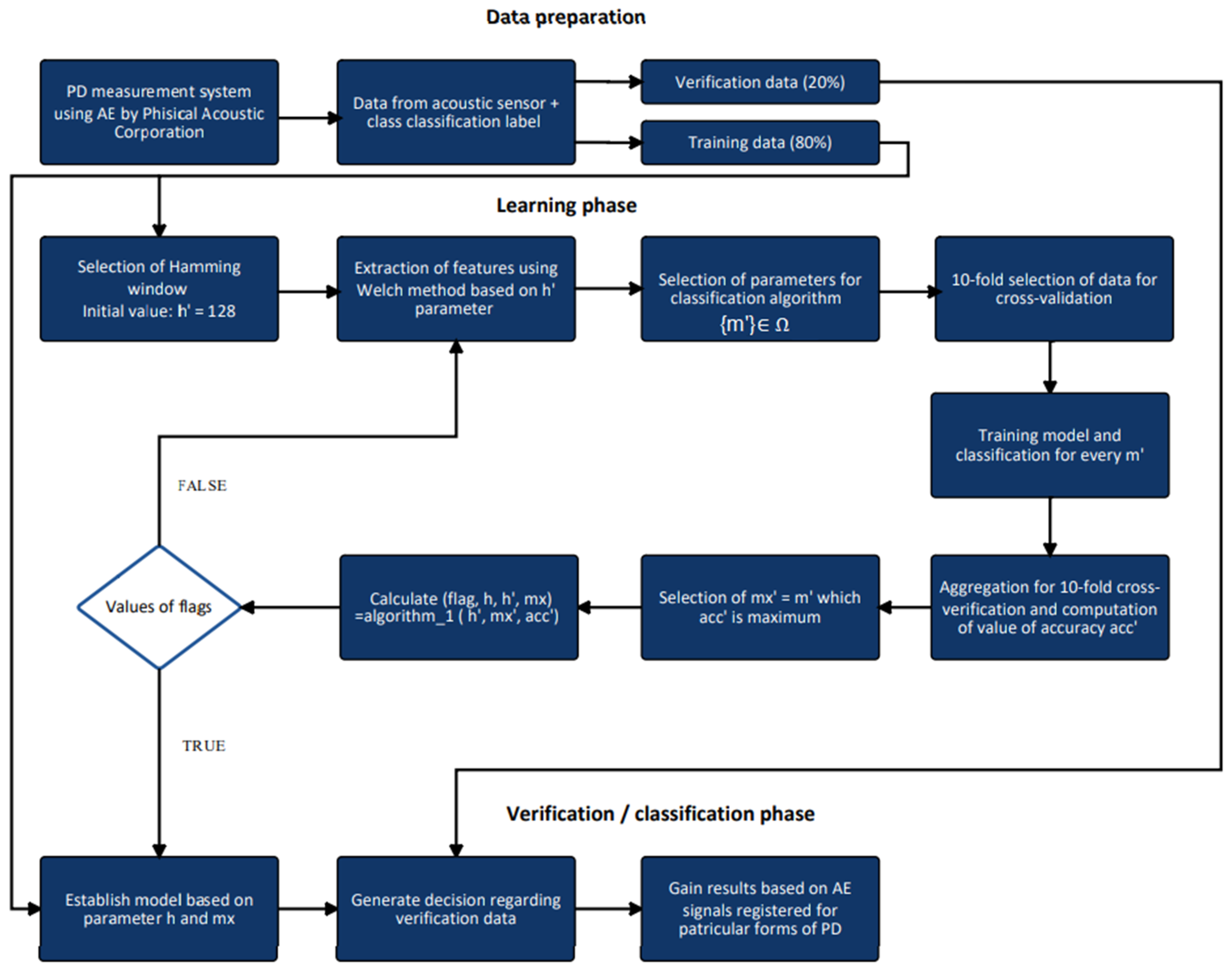
The application of three various types of core parts was investigated as part of the current research; however, the linear and radial core turned out to be ineffective, and the accuracy was below 50%, therefore further research focused on the polynomial core. However, preliminary studies have shown that the data is susceptible to classification and it is possible to obtain a high level of classification of particular forms of PD at the initial stage. On the basis of the preliminary analysis, a method based on the frequency analysis and classifiers were proposed, which will make it possible to obtain a high level of classification, taking into account the computational complexity by reducing the number of input features. An algorithm of the proposed approach is presented in Figure 4.
In the first stage, sound signals are registered with a sensor dedicated for this purpose. These datasets are presented as time series X = [x1, x2,…, xn], where n is the number of samples. In the next step, the time series X was transformed into a frequency domain vector, using the Welch method to reduce the size of the sample. The initial value of the Hamming window has been set at h′ = 128 on the basis of preliminary data. Subsequently, the analysis involved the impact of the Hamming window value on the classification result depending on the type of classifier that was utilized. The parameters of the tuned model { m }   Ω differs depending on the type of the classifier and it can contain from zero to multiple parameters. Each loop searches for optimal parameters set for one Hamming window width only. The parameters are selected by an exhaustive search in a parallel process. It is important that the classifier is tuned to fit for one Hamming window width. The obtained accuracy of the classification (acc′) is used to optimize the parameters and is a function that is maximized. This accuracy is defined as:
a c c = T P + T N T P + T N + F P + F N ,
where TP is true positive (correct classification), TN is true negative (correct rejection), FP is false negative (error type I) and FN is false negative (error type II).
Following the reception of optimization result of the mx parameter (described below), a decision is made whether a further tuning of the parameters is needed or it can be terminated in accordance with the procedure specified below (Algorithm 1):
Algorithm 1
1. Get current values of acc′, mx′, h′.
2. IF first algorithm iteration:
  a. direction = 1; step = 0; op = 0
  b. acc = acc′, mx = mx′, h = h′, h′ = h′*2;
  c. IF acc == 100 THEN direction = 3 and goto 5.
  d. flag = FALSE and goto point 6.
3. IF direction == 1 THEN
  a. IF acc′ > acc THEN FLAG = FALSE, step = 0, h = h′, h′ = h′*2, acc = acc′,
  mx = mx′, op = 1
  b. IF acc′ == acc THEN FLAG = FALSE , step++, h′ = h′*2,
  c. IF acc′ < acc THEN FLAG = FALSE and direction = 3,
  d. IF step == 2 THEN direction = 3,
4. IF direction == 2 THEN
  a. IF acc′ >= acc THEN FLAG = FALSE, h = h′, h′ = h′/2, acc = acc′, mx = mx′,
  b. ELSE FLAG = TRUE
5. IF direction == 3 THEN
  a. IF op ==1 THEN FLAG = TRUE and goto point 6
  b. ELSE h′ = h/2, direction = 2;
6. Return flag and h′.
The proposed algorithm constitutes a derivative of the hill climbing [48] strategy. The modification allows the searching of optimal model parameters to speed up when the classifier model accuracy is close to or equal to 100%. The algorithm in the first phase maximizes model accuracy (direction equals 1) and, in the second phase, optimizes Hamming window width (direction equals 2) to reduce size of input data for the classifier model. Additionally, it verifies Hamming window length two steps ahead to make the solution more robust.
By default, in hill climbing, a random start combination is created and the direct neighbors are evaluated (respecting the given intervals and step sizes). The best combination among the neighbors is the start point for the next iteration. If no neighbor improves the objective function the loop terminates. The algorithm for the first iteration (step 2) preserves the parameters and enlarges the Hamming window and continues loops (flag = FALSE). In the first phase of the algorithm (direction == 1 for point 3), the Hamming window is increased as long as the accuracy increases (3a), and two steps ahead are verified to see if its value does not increase further (3b). The algorithm terminates when the detection accuracy drops or does not increase within two steps. Before it is complete, a case is verified to see if the accuracy could not be increased from the initial phase (steps 5 and 2). If the value in the first step assumed the maximum, there is a need to verify whether it is possible to obtain the same result by use of a smaller window. Ultimately, after the algorithm is terminated, parameters are established to fulfil the condition in which case the accuracy is the highest and the window is minimized as much as possible in order to reduce computational complexity.
The machine learning model M was derived on the basis of the mx parameters of a given model and a set of features, the number of which is determined by the Hamming window (h). A number of ML algorithms were tested to verify their applicability for this purpose. These include the k-nearest neighbors (KNN) algorithm, decision trees, multi-layer perceptron network (MLP), classical support vector machines (SVM) and the Bayes approach. The KNN method classifies a new data vector by looking at the k data vectors closest to it in the feature domain. In the proposed method, the Euclidean distance and the number of the nearest neighbors were chosen as the parameter mx ∈ Ω, mx = [k], k∈ [3, …, 12]. In the case of probabilistic classifiers, there is a possibility of using the ones that identify a naive Bayesian family on the basis of the Bayes theorem with the assumption of independence between features, and, therefore, no parameters are required. The aim of using SVM machines and non-probabilistic approach is to identify the hyperplanes that separate the search classes. In this study, the SVM kernel was used, which finds a hyperplane that is represented by a polynomial function of the input features. In the case of the core, the following parameters are trained: power value, bias and gamma parameter (mx ∈ Ω, mx = [p, b, g], p, b, g = [0.4, 0.5, …, 1.6]). In the case of the random forest (RF) method, where many trees are trained instead of training one tree, the number of trees was determined as the parameter mx ∈ Ω, mx = [t], t ∈ [1, …, 12]. On the basis of preliminary studies, the maximum number of trees was set at 12. Above this level, no improvement in accuracy was established. The PNN was selected to be representative of the artificial neural network. It turned out to be adequate for the classification tasks. In this case, the following parameters were taken into account: theta minus and theta plus (mx ∈ Ω, mx = [tm, tp], tm = [0.1, 0.2, …, 0.6], tp = [0.2, 0.3, …, 1.2], tm < tp).

4. Results and Discussion

The tuning of the methods for specific algorithms was conducted in accordance with the procedure presented in Figure 4. A tuning example was presented for the kNN method. According to the algorithm, the tuning was started for h′ = 128 (Table 2). The underlined results show the initial (reference) values obtained on the basis of preliminary tests. The results in bold are the elements for which the optimal accuracy was achieved, selected by Algorithm 1.
Throughout the third step for h′ = 512, the accuracy of the model was established at a level of 99.6%. Despite the increasing of the window width by two times, a further increase in the accuracy was not gained.
Similar tuning was performed for the SVM model where the tuning required the use of as many as three parameters. These steps are presented in Table 3.
The model assumed its maximum value already in the first step. Therefore, in the second part of the algorithm, the window width was reduced. Shrinking the window for the next iteration decreased accuracy so the algorithm was terminated. In the same manner, the algorithm was fine tuned for the other classifiers. The algorithm verification results for the final model are presented in Table 4.
The results of the classification demonstrate that for both the kNN and SVM models that applied tuning by application of the proposed algorithm offer 100% efficiency for detection for all eight classes. It has been observed that the SVM model behaved more stable during the tuning, as presented in Table 4. In the case of the kNN model, it is equally effective; however, four times more data is required to gain a solution. It can be concluded that the tuned polynomial planes are most suitable to the analyzed data. In the case of the other classifiers, a high efficiency of 97.8% and 97.2% was obtained for the Bayesian classifier and the decision trees (RF), respectively. The effectiveness of inference is presented in Table 5 and Table 6.
The results demonstrate that classes 1, 2 and 7 are recognized by both classifiers without any problems. The biggest problems can be identified in the use of classes from 4 to 6. These can be attributable to the greater similarity of these classes among each other. Similar results can be noticed for the PNN classifier, the results of which are presented in Table 7.
The PNN classifier identifies classes 1, 2 and 7 class the highest sensitivity; however in case of nine examples they were falsely classified as class 1. In contrast, in class 6, nine values were classified as false negative. The future improvement for this classifier involves an increase of this two-class distinction.

5. Conclusions

The proposed method using the acoustic emission signals allows researchers to obtain data which are prone to proposed machine learning methods. This is the next step in the development of automated non-invasive methods of diagnostics of power devices based on acoustic emission methods for the assessment of the technical condition of high-voltage insulation systems of power devices in terms of detection, location and identification of partial discharges. Despite the classical approach, the data characteristics achieve a level of high accuracy; thus, in this paper the focus was to find the minimal and optimal hamming window that will produce reliable classification. In experiments, the optimal window of 128 for the SVM algorithm and 512 in case of the kNN algorithm were selected.
The proposed approach allows researchers to decrease the number of samples by decreasing the Hamming window. The results show that a window of length 1024 was sufficient in most cases. The best results were achieved using SVM classified tuned with polynomial core, and obtained 100% accuracy. Similar results were achieved with the kNN classifier; however, a four times greater window was required. Finally, random forest and naïve bayes obtained high accuracy over 97%. It is worth noting that the Bayes classifier does not need parameters to tune. Finally, the PNN network obtained an average result of 92%. This classifier is not recommended due to a long training and tuning process.
Raymond et al. [49] reached similar conclusions in their publication, choosing the SVM classifier as one of the best for this task. The manuscript also describes the PNN method as the next solution in the classification of PD. In turn, Barrios et al. [50] have focused on the use of deep learning (DL) methods for the automated identification of PD. The main conclusions have demonstrated that Deep Neural Networks (DNN) have better accuracy than typical ML methods, providing more efficient automated identification techniques. However, the processing stage and classifying time is longer and more complex.
Due to the simplicity of our approach and the low complexity of the trained model, it can be applied in real-time systems, which means that the process of identifying, classifying and associating the registered PDs with a given type of defect can be performed immediately, which in turn enables “on-line” diagnostic measurements to be performed to assess the condition of the tested insulation.

Author Contributions

Conceptualization, T.B. and S.B.; Methodology, P.K., D.J. and M.B.; Software, M.B., D.J. and T.B.; Validation, S.B. and P.K.; Formal Analysis, T.B. and S.B.; Investigation, S.B., P.K., D.J., M.B. and T.B.; Writing—Original Draft Preparation, S.B., M.B. and D.J.; Writing—Review and Editing, P.K., D.J., T.B., M.B. and S.B. All authors have read and agreed to the published version of the manuscript.

Funding

This research received no external funding.

Informed Consent Statement

Informed consent was obtained from all subjects involved in the study.

Conflicts of Interest

The authors declare no conflict of interest.

References

  1. Mirzaei, H.; Akbari, A.; Gockenbach, E.; Miralikhani, K. Advancing new techniques for UHF PD detection and localization in the power transformers in the factory tests. IEEE Trans. Dielectr. Electr. Insul. 2015, 22, 448–455. [Google Scholar]
  2. Murugan, R.; Ramasamy, R. Failure analysis of power transformer for effective maintenance planning in electric utilities. Eng. Fail. Anal. 2015, 55, 182–192. [Google Scholar] [CrossRef]
  3. Takahashi, R.H.C.; Diniz, H.E.P.; Carrano, E.G.; Campelo, F.; Batista, L.S. Multicriteria transformer asset management with maintenance and planning perspectives. IET Gener. Transm. Distrib. 2016, 10, 2087–2097. [Google Scholar]
  4. Boczar, T.; Cichon, A.; Borucki, S. Diagnostic expert system of transformer insulation systems using the acoustic emission method. IEEE Trans. Dielectr. Electr. Insul. 2015, 21, 854–865. [Google Scholar] [CrossRef]
  5. Fuhr, J. Procedure for identification and localization of dangerous partial discharges sources in power transformers. IEEE Trans. Dielectr. Electr. Insul. 2005, 12, 1005–1014. [Google Scholar] [CrossRef]
  6. Rubio-Serrano, J.; Rojas-Moreno, M.V.; Posada, J.; Martienez-Tarifa, J.M.; Robles, G.; Garcia-Souto, J.A. Electro-acoustic detection, identification and location of PD sources in oil-paper insulation systems. IEEE Trans. Dielectr. Electr. Insul. 2012, 19, 1569–1578. [Google Scholar] [CrossRef]
  7. Boczar, T. Identification of a specific type of PD form acoustics emission frequency spectra. IEEE Trans. Dielectr. Electr. Insul. 2001, 8, 598–606. [Google Scholar] [CrossRef]
  8. Borucki, S.; Łuczak, J.; Zmarzły, D. Using Clustering Methods for the Identification of Acoustic Emission Signals Generated by the Selected Form of Partial Discharge in Oil-Papier Insulation. Arch. Acoust. 2018, 43, 207–215. [Google Scholar]
  9. Castro Heredia, L.C.; Rodrigo Mor, A. Density-based clustering methods for unsupervised separation of partial discharge sources. Int. J. Electr. Power Energy Syst. 2019, 107, 224–230. [Google Scholar]
  10. Boczar, T.; Borucki, S.; Cichoń, A.; Zmarzły, D. Application Possibilities of Artificial Neural Networks for Recognizing Partial Discharges Measured by the Acoustic Emission Method. IEEE Trans. Dielectr. Electr. Insul. 2009, 16, 214–223. [Google Scholar] [CrossRef]
  11. Boczar, T.; Borucki, S.; Cichoń, A.; Lorenc, M. Recognizing partial discharge forms measured by the acoustic emission method using the spectrum power density as a parameter of the artificial neuron network. Mol. Quantum Acoust. Annu. J. 2005, 26, 35–44. [Google Scholar]
  12. Kurtasz, P.; Boczar, T. The application of the optimized multicomparative algorithm for classifying acoustic signals, generated by partial discharges, cataloged in the modified database. Meas. Autom. Robot. 2010, 12, 73–79. [Google Scholar]
  13. Barber Bayesian, D. Reasoning and Machine Learning; Cambridge University Press: Cambridge, UK, 2012. [Google Scholar]
  14. Mahdavinejad, M.S.; Rezvan, M.; Barekatain, M.; Adibi, P.; Barnaghi, P.; Sheth, A.P. Machine learning for internet of things data analysis: A survey. Digit. Commun. Netw. 2018, 4, 161–175. [Google Scholar] [CrossRef]
  15. Murphy, K.P. Machine Learning: A Probabilistic Perspective; MIT Press: Cambridge, MA, USA, 2012. [Google Scholar]
  16. Cunningham, P.; Delany, S.J. K-nearest neighbour classifiers. Mult. Classif. Syst. 2007, 34, 1–17. [Google Scholar]
  17. Cortes, C.; Vapnik, V. Support-vector networks. Mach. Learn. 1995, 20, 273–297. [Google Scholar] [CrossRef]
  18. Scholkopf, B.; Smola, A.J. Learning with Kernels: Support Vector Machines, Regularization, Optimization, and Beyond; MIT Press: Cambridge, MA, USA, 2001. [Google Scholar]
  19. Breiman, L. Random forests. Mach. Learn. 2001, 45, 5–32. [Google Scholar]
  20. Breiman, L. Bagging predictors. Mach. Learn. 1996, 24, 123–140. [Google Scholar] [CrossRef] [Green Version]
  21. He, K.; Zhang, X.; Ren, S.; Sun, J. Deep Residual Learning for Image Recognition. In Proceedings of the IEEE Conference on Computer Vision and Pattern Recognition, Las Vegas, NV, USA, 27–30 June 2016; pp. 770–778. [Google Scholar]
  22. Eberhart, R.C. Neural Network PC Tools: A Practical Guide; Academic Press: Cambridge, MA, USA, 2014. [Google Scholar]
  23. Glorot, X.; Bengio, Y. Understanding the difficulty of training deep feedforward neural networks. In Proceedings of the 13th International Conference Artificial Intelligence and Statistics (AISTATS), Sardinia, Italy, 13–15 May 2010; pp. 249–256. [Google Scholar]
  24. Ziółkowski, J.; Oszczypała, M.; Małachowski, J.; Szkutnik-Rogoż, J. Use of Artificial Neural Networks to Predict Fuel Consumption on the Basis of Technical Parameters of Vehicles. Energies 2021, 14, 2639. [Google Scholar] [CrossRef]
  25. LeCun, Y.; Bengio, Y.; Hinton, G. Deep learning. Nature 2015, 521, 436–444. [Google Scholar] [CrossRef]
  26. Abdi, H.; Williams, L.J. Principal component analysis. Wiley Interdiscip. Rev. Comput. Stat. 2010, 2, 433–459. [Google Scholar] [CrossRef]
  27. Bro, R.; Smilde, A.K. Principal component analysis. Anal. Methods 2014, 6, 2812–2831. [Google Scholar] [CrossRef] [Green Version]
  28. Hotelling, H. Analysis of a complex of statistical variables into principal components. J. Educ. Psychol. 1933, 24, 417. [Google Scholar] [CrossRef]
  29. Jollie, I. Principal Component Analysis; Wiley Online Library: Hoboken, NJ, USA, 2002. [Google Scholar]
  30. Bach, F.R.; Jordan, M.I. Kernel independent component analysis. J. Mach. Learn. Res. 2002, 3, 1–48. [Google Scholar]
  31. Hotelling, H. Relations between two sets of variates. Biometrika 1936, 28, 321–377. [Google Scholar] [CrossRef]
  32. Keerthi, S.S.; Shevade, S.K.; Bhattacharyya, C.; Murthy, K.R.K. Improvements to Platt’s SMO Algorithm for SVM Classifier Design. Neural Comput. 2001, 13, 637–649. [Google Scholar] [CrossRef]
  33. Platt, C. Sequential Minimal Optimization: A Fast Algorithm for Training Suppor Vector Machines. In Advances in Kernel Methods-Support Vector Learning; MIT Press: Cambridge, MA, USA, 1999; pp. 185–208. [Google Scholar]
  34. Aha, D.W.; Kibler, D.; Albert, M.K. Instance-based learning algorithms. Mach. Learn. 1991, 6, 37–66. [Google Scholar] [CrossRef] [Green Version]
  35. De Lautour, O.R.; Omenzetter, P. Damage classification and estimation in experimental structures using time series analysis and pattern recognition. Mech. Syst. Signal Process. 2010, 24, 1556–1569. [Google Scholar] [CrossRef] [Green Version]
  36. Zhang, H. The optimality of naive bayes. AA 2004, 1, 3. [Google Scholar]
  37. Rabiner, L.R. A tutorial on hidden markov models and selected applications in speech recognition. Proc. IEEE 1989, 77, 257–286. [Google Scholar] [CrossRef] [Green Version]
  38. Sejnowski, T.J.; Rosenberg, C.R. Parallel networks that learn to pronounce english text. Complex Syst. 1987, 1, 145–168. [Google Scholar]
  39. Kalman, R.E.; Bucy, R.S. New results in linear filtering and prediction theory. J. Basic Eng. 1961, 83, 95–108. [Google Scholar]
  40. Laerty, J.; McCallum, A.; Pereira, F. Conditional random fields: Probabilistic models for segmenting and labeling sequence data. In Proceedings of the Eighteenth International Conference on Machine Learning, ICML, Williamstown, MA, USA, 28 June–1 July 2001; Volume 1, pp. 282–289. [Google Scholar]
  41. Williams, R.J.; Zipser, D. A learning algorithm for continually running fully recurrent neural networks. Neural Comput. 1989, 1, 270–280. [Google Scholar] [CrossRef]
  42. Baltrušaitis, T.; Ahuja, C.; Morency, L. Multimodal Machine Learning: A Survey and Taxonomy. IEEE Trans. Pattern Anal. Mach. Intell. 2018, 41, 423–443. [Google Scholar] [CrossRef] [Green Version]
  43. McCallum, A.; Freitag, D.; Pereira, F. Maximum Entropy Markov Models for Information Extraction and Segmentation. In Proceedings of the 17th International Conference on Machine Learning, ICML, Stanford, CA, USA, 29 June–2 July 2000; Volume 17, pp. 591–598. [Google Scholar]
  44. Welch, P. The use of fast Fourier transform for the estimation of power spectra: A method based on time averaging over short, modified periodograms. IEEE Trans. Audio Electr. 1967, 15, 70–73. [Google Scholar] [CrossRef] [Green Version]
  45. Jancarczyk, D.; Bernaś, M.; Boczar, T. Classification of Low Frequency Signals Emitted by Power Transformers Using Sensors and Machine Learning Methods. Sensors 2019, 19, 4909. [Google Scholar] [CrossRef] [PubMed] [Green Version]
  46. Jancarczyk, D.; Bernaś, M.; Boczar, T. Distribution Transformer Parameters Detection Based on Low-Frequency Noise, Machine Learning Methods, and Evolutionary Algorithm. Sensors 2020, 20, 4332. [Google Scholar] [CrossRef]
  47. Berthold, M.R.; Cebron, N.; Dill, F.; Gabriel, T.R.; Tobias, K.; Meinl, T.; Ohl, P.; Sieb, C.; Thiel, K.; Wiswedel, B. KNIME: The Konstanz Information Miner. In Data Analysis, Machine Learning and Applications. Studies in Classification, Data Analysis, and Knowledge Organization; Preisach, C., Burkhardt, H., Schmidt-Thieme, L., Decker, R., Eds.; Springer: Berlin/Heidelberg, Germany, 2008. [Google Scholar]
  48. Selman, B.; Gomes, C.P. Hill-climbing search. In Encyclopedia of Cognitive Science; John Wiley: Hoboken, NJ, USA, 2006. [Google Scholar]
  49. Raymond, W.J.K.; Illias, H.A.; Bakar, A.H.A.; Mokhlis, H. Partial discharge classifications: Review of recent progress. Measurement 2015, 68, 164–181. [Google Scholar] [CrossRef] [Green Version]
  50. Barrios, S.; Buldain, D.; Comech, M.P.; Gilbert, I.; Orue, I. Partial Discharge Classification Using Deep Learning Methods—Survey of Recent Progress. Energies 2019, 12, 2485. [Google Scholar] [CrossRef] [Green Version]
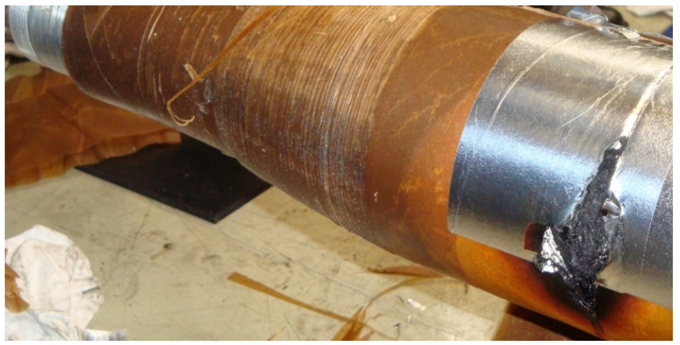
Figure 1. Example of a failure in the paper-oil insulation system of a 220 kV insulator bushing due to uncontrolled development of surface PD.
Energies 15 05013 g001
Figure 2. Example of a catastrophic failure of a transformer due to an explosion of an insulator bushing caused by internal PD.
Energies 15 05013 g002
Figure 3. Example of collective frequency analysis of AE signals registered for particular analyzed classes of PDs.
Energies 15 05013 g003
Figure 4. Block diagram of proposed algorithm applied for classification of AE signals depending on PD forms.
Energies 15 05013 g004
Table 1. Initial analysis of the spectrum of the recorded AE signals from PD executed for different widths of the Hamming window for various classifiers and ten-fold cross-validation.
Accuracy [%]
Hamming
Window
KNNSVMRandom TreesBayesPNN
819299.399.997.398.291.4
409699.399.997.798.191.5
204899.299.998.698.291.3
102499.199.998.998.291.4
51299.199.997.497.891.4
25698.999.998.797.791.8
12898.810098.397.789.7
6498.499.997.29687.9
3297.699.897.494.884.4
1696.19896.693.879
891.190.29389.872
490.479.390.187.363.3
288.760.587.986.459.8
170.230.964.370.267.3
Table 2. Subsequent steps of algorithm applied in search of an optimum parameter for method to select kNN.
k (Accuracy)
It.h′3456789101112
112899.299.39998.998.598.597.398.397.997.6
2256999999.29999.298.398.598.398.398.2
351299.699.499.39999.298.398.298.398.398.1
410249999.298.998.998.698.998.998.698.698.6
5204899.499.599.399.298.798.998.898.898.598.5
Table 3. Optimization of parameters in the case of SVM model.
SVM
It.h′PBgAcc
1a1281.20.60.6100
1b12811.40.6100
2a640.60.60.699.9
2b640.610.699.9
2c6410.60.899.9
Table 4. Classification of PD classes using the proposed model.
ML MethodML Method ParametersTrainingAccuracyCohen Cappa
kNNh = 512, k = 399.7%100%100%
naive Bayesh = 102498.2%97.8%97.5%
MLPh = 256,
tm = 0.2, tp = 0.4
91.4%92.2%91.1%
RFh = 128, t = 1298.4%97.2%96.8%
SVMh = 128, p = 1.2, b = 0.6, g = 0.6100%100%100%
KNN: k-Nearest Neighbors; naïve Bayes: Naive Bayes Classification; MLP: Multiple Layer Perceptron Network; RF: Random Forests; SVM: Support Vector Machine.
Table 5. Results of classification of eight investigated classes of PDs that applied Bayes classifier.
ClassTrue
Positive
False
Positive
True
Negative
False
Negative
RecallAccuracySensitivitySpecificityf-Measure
1220157196%100%96%100%98%
22301570100%100%100%100%100%
32301570100%100%100%100%100%
4211157195%95%95%99%95%
5202157195%91%95%99%93%
6182158290%90%90%99%90%
7223153292%88%92%98%90%
8230156196%100%96%100%98%
Table 6. Results of classification of eight investigated classes of PDs that applied Random Forest classifier.
ClassTrue
Positive
False
Positive
True
Negative
False
Negative
RecallAccuracySensitivitySpecificityf-Measure
1220157196%100%96%100%98%
22301570100%100%100%100%100%
32301570100%100%100%100%100%
42221560100%92%100%99%96%
5190159290%100%90%100%95%
6190160195%100%95%100%97%
72421540100%92%100%99%96%
82401560100%100%100%100%100%
Table 7. Results of classification of eight investigated classes of PDs using PNN classifier.
ClassTrue
Positive
False
Positive
True
Negative
False
Negative
RecallAccuracySensitivitySpecificityf-Measure
1221156196%96%96%99%96%
22391480100%72%100%94%84%
32311560100%96%100%99%98%
4211157195%95%95%99%95%
5201158195%95%95%99%95%
6181159290%95%90%99%92%
7150156963%100%63%100%77%
82401560100%100%100%100%100%
Publisher’s Note: MDPI stays neutral with regard to jurisdictional claims in published maps and institutional affiliations.