Article

Combining Deep Learning and the Heat Flux Method for In-Situ Thermal-Transmittance Measurement Improvement

by
Sanjin Gumbarević
1,*,
Bojan Milovanović
2,
Bojana Dalbelo Bašić
3 and
Mergim Gaši
2
1
Ericsson Nikola Tesla, Krapinska 45, 10000 Zagreb, Croatia
2
Faculty of Civil Engineering, University of Zagreb, 10000 Zagreb, Croatia
3
Faculty of Electrical Engineering and Computing, University of Zagreb, 10000 Zagreb, Croatia
*
Author to whom correspondence should be addressed.
Energies 2022, 15(14), 5029; https://doi.org/10.3390/en15145029
Submission received: 11 May 2022 / Revised: 1 July 2022 / Accepted: 6 July 2022 / Published: 9 July 2022
(This article belongs to the Special Issue Optimization and Innovation of Nearly Zero-Energy Buildings)

Abstract

:
Transmission losses through the building envelope account for a large proportion of building energy balance. One of the most important parameters for determining transmission losses is thermal transmittance. Although thermal transmittance does not take into account dynamic parameters, it is traditionally the most commonly used estimation of transmission losses due to its simplicity and efficiency. It is challenging to estimate the thermal transmittance of an existing building element because thermal properties are commonly unknown or not all the layers that make up the element can be found due to technical-drawing information loss. In such cases, experimental methods are essential, the most common of which is the heat-flux method (HFM). One of the main drawbacks of the HFM is the long measurement duration. This research presents the application of deep learning on HFM results by applying long-short term memory units on temperature difference and measured heat flux. This deep-learning regression problem predicts heat flux after the applied model is properly trained on temperature-difference input, which is backpropagated by measured heat flux. The paper shows the performance of the developed procedure on real-size walls under the simulated environmental conditions, while the possibility of practical application is shown in pilot in-situ measurements.

1. Introduction

The majority of buildings that exist today are expected to still exist in the next 50 years [1,2]. Thus, it is clear that a large number of buildings will require extensive energy retrofits to achieve required energy-efficiency levels [3]. This is one of the main reasons why the construction industry is seen as a sector where energy-saving measures can be implemented to reduce environmental impacts [4,5]. Even though the primary goal of the environmental performance of buildings is related to greenhouse-gas emissions, the thermal performance of a building must still be considered as a key factor, as improving the energy efficiency of a building will reduce greenhouse-gas emissions [6,7,8]. Energy goals should not take precedence over occupant well-being. Therefore, it is important to design building envelopes to achieve both goals. For this reason, design solutions for both new and retrofitted buildings must follow a holistic vision of the building sector, where professionals are confronted with a contrast between reality and historical traditions, and environmental and cultural considerations, while applying new concepts of sustainability, biocompatibility, energy conservation and the use of renewable resources [9,10,11]. This is even more important when it comes to the retrofit of historic buildings [12,13]. When it comes to improving the thermal performance of the building envelope, the most common method is to limit the thermal transmittance (U-value) of the envelope element [14,15,16]. The U-value is defined as the reciprocal of the total thermal resistance of the element, which is the thermal resistance per unit temperature, i.e., the U-value is a measure of how much heat flows through an element per unit temperature [17]. Estimating transmission losses of the envelope elements of existing buildings is challenging due to the potential degradation of thermal properties, the effects of heterogeneity in the elements, and the effects of moisture [18,19,20]. In the case of such an assessment for existing buildings, one of four experimental in-situ methods should be used to determine the U-value: the heat-flux method (HFM), the thermometric method, the HFM with hot box, or quantitative infrared thermography [17,20,21].There are two main reasons why it is important to estimate the U-value as close to reality as possible—we can decide on measures that lead to poor energy efficiency (optimistic U-value estimation) and those that lead to unnecessary measures, which are usually quite expensive (pessimistic U-value estimation). Of the listed methods, only the HFM method is a standardized method according to ISO 9869-1 [22] for the in-situ determination of the U-value, and is widely used not only for engineering purposes but also in academic research [20,23], as shown in Figure 1.
HFM uses a sensor to measure heat flux and two thermocouples to measure indoor and outdoor air temperature. The U-value is calculated using one of two proposed standardized post-processing methods based on the two observed temperatures and a heat flux: from the average of the recorded values (mean value method) or using the transformations in the heat-conduction equation (dynamic method). For the results of the in-situ test to be meaningful, the test must be performed when the element is under conditions of a high-intensity temperature gradient [24,25], i.e., the analyzed element must be between temperature differences that result in a non-zero heat flux [26]. This is especially important for well-insulated elements, since such elements resist heat flow. Therefore, a stronger temperature gradient must be applied to register a relevant heat flux. If the element is not under condition of a high-intensity temperature gradient, there is a high probability that a significant deviation from the predicted U-value (with deviations greater than 80% [27]) will occur. This condition must be met by three of the four listed in-situ U-value methods, all except HFM with hot box [20]. When the described condition is met, then the maximum deviation in the U-value is usually limited to a maximum value of about 20% relative difference with respect to the theoretical U-value [28,29], this U-value is calculated using the standard ISO 6946 [30]. In addition to the above, in order to obtain reliable results, it is important that the boundary conditions in the indoor spaces are kept as steady as possible to the constant temperature [31]. Furthermore, the reliability of the results is affected by stochastically determined outdoor conditions (rain, sun) and large temperature variations [32].
When all these unfavorable conditions occur, measurement is prolonged because they affect the stability criteria of the standard [22], so the duration of the test can be prolonged to more than 2 weeks [20,31,32]. The extension of the measurement duration is mainly influenced by the decrease in the temperature gradient and the oscillation of the indoor temperature [33]. Since the outdoor boundary condition is the outdoor air temperature and the indoor boundary condition is a constant temperature affected by occupants, the measurement duration can be shortened by parallelization. We can measure more than one element at a time with multiple HFM devices, but this way is financially and operationally inefficient [34]. On the other hand, there are examples in the literature of shortening the measurement time by applying artificial-intelligence (AI) models to the results to predict the resulting U-value based on in-situ methods [35,36,37,38,39].
Although the history of AI dates back to the early beginnings of computer science, it came into focus in the last decade due to significant improvements in computer hardware and the development of new algorithms [40,41]. Machine learning (ML), as a subfield of AI, is increasingly applied to sensor results [42], where these results serve either as input data for prediction or for classification of the observed phenomenon. These results can also serve as a data set on which the ML model learns. For example, it is possible to create an ML model based on data obtained by numerical analysis of the solution to the heat equation. In this way, the ML model was created in [39], which achieved a relative difference for the predicted thermal resistance (reciprocal of thermal transmittance) of less than 10% compared to the thermal resistance obtained using the standardized HFM test. This methodology was tested on four types of walls under controlled environmental conditions. Similarly, the ML model can be developed by using a set of boundary conditions and thermal properties as input, so that the model predicts the thermal transmittance by backpropagation and compares the output of the model with the measured value based on the thermometric measurement. In this way, a maximum difference from the expected value of about 20% can be obtained [35]. On the other hand, the HFM results can also be used as a data set for training the ML model, which predicts the heat flux on a set of unseen data after a satisfactory prediction has been achieved. These predicted heat-flux time series are then used to determine the U-value. The models from [37,38] have two input parameters—outdoor and indoor air temperature—and the resulting heat flux is predicted. In this case, differences from 0.78% to 8.73% can be obtained with respect to HFM measurements. However, the article [37] does not show how the typology and architecture of the neural network was determined, and the application was developed only for one wall.
This paper investigates whether deep learning can be applied to HFM results to shorten the usage of the HFM sensor in determining the U-value by HFM in-situ measurement. The paper also shows an analysis of conditions such as registration of a low-temperature gradient or near-zero heat flux. The HFM method was chosen because it is the most commonly used, as can be seen in Figure 1. In addition to this section, the paper consists of four other sections. In the Section 2, Materials and Methods, the knowledge behind HFM and deep learning is analyzed in detail and the research design is presented. Section 3, Results, shows the application of deep-learning models to a heat-flux prediction regression problem, and Section 4, Discussion, analyzes these results in detail. Finally, Section 5, Conclusion, presents the general findings from this research.

2. Materials and Methods

The research methodology follows simple steps of data collection according to the standard ISO 9869-1 [22], formation of deep-learning regression model, analysis of prediction results and comparison with theoretical U-value defined according to the standard ISO 6946 [30]. This section consists of four subsections that define all the knowledge needed to understand the experimental setup and the methods used for the research. Section 2.1 explains the way to calculate the theoretical U-value as well as the theoretical background of the U-value, while Section 2.2 shows the knowledge and procedures for the in-situ HFM test. Since this paper shows the application of deep-learning HFM results, Section 2.3 presents the general knowledge needed to understand the background of the developed models. At the end of the section (Section 2.4), the experimental setup is presented and the methodology of the research is described in detail.

2.1. Theoretical U-Value

When we consider a one-dimensional heat flux through a single-layer element, the heat flux at steady state can be defined by a combination of the solution of the heat-flux equation and Fourier’s law of heat conduction:
q = λ T i n t e r i o n r T e x t e r i o r d i . e . , q = T i n t e r i o r T e x t e r i o r R ,
where q is the heat flow rate in W / m 2 , λ is the thermal conductivity in W / ( m K ) , d is the thickness of the element in m, R = d / λ is the thermal resistance in m 2 K/W, and T e x t e r i o r and T i n t e r i o r are the temperatures of the exterior and interior environment in °C or K, respectively. If we have more than one layer in an element, then the thermal resistance of an element can be calculated in the following way:
R = i = 1 n d i λ i .
For the total thermal resistance ( R T ) for a heat flow from the internal environment through an element to the external environment, we need to add the thermal resistance of the internal surface ( R s i ) and the thermal resistance of the external surface ( R s e ) to the expression (2) so that it is defined as R T = R s i + R + R s e . R s i and R s e can be defined by Table 1 of the standard ISO 6946 [30]. The U-value is defined as the reciprocal of the total thermal resistance ( U = 1 / R T ), so the heat flow rate is defined as follows:
q = U ( T i n t T e x t ) .
Since the expression (3) defines the heat-flux estimate in a simple way, the U-value has recently become the most common method for classifying building elements when considering their thermal performance. When comparing with the numerically solved heat equation for the same element, overestimates and underestimates of heat flux occur because steady-state conditions never exist in reality [43]. Policy measures often limit the U-values of building elements, but when we solve a problem of great importance, it is better to analyze the problem with numerical methods, since dynamic parameters such as heat storage are included in the analysis, so that we can, for example, optimize the thickness of the insulation layer so that we have a larger U-value but better energy efficiency when considered all year round [44]. All results are compared with the U-value defined in this subsection, since the analyzed specimens from the experimental research have known layers and it is common in the literature ([23,27,33,45,46,47]) to compare the analyzed solution with the theoretical U-value defined in this way.

2.2. Heat-Flux Method

Since the thermal transmittance (U-value) is the rate of heat flow at steady state divided by the area and by the temperature difference of an element at the boundary between two environments, it is difficult to determine it in situ, since these conditions never occur. This difficulty can be overcome by assuming that the averages of the temperatures and the heat flux give a good estimate of the steady state. This assumption is valid if the following conditions are met, according to ISO 9869-1 [22]:
  • The heat transfer coefficients and thermal properties of the materials are constant under actual ambient conditions during the test.
  • The heat storage effect is negligible. This usually results in long measurement periods.
The main instrument for measuring heat flux according to ISO 9869-1 is the heat flux sensor. It is essentially a transducer that provides an electrical signal directly related to the heat flux transmitted through the sensor. The sensor is a thermally resistant plate connected to the data logger in such a way that it can be easily moved. It must have low thermal resistance to ensure that it does not have a large effect on the heat flux, and high sensitivity so that it can register a sufficient signal value at low heat-flux rates. When installing the sensor on the measuring element, it is recommended that no material be used between the element and the sensor, because even though this is theoretically permissible; in reality, it will result in relative differences by more than 20% when comparing the measured U-value with the expected [45]. In addition to the heat-flux sensor, the device for standardized U-value measurement contains two temperature sensors for measuring outdoor and indoor temperatures. These are transducers that register an electrical signal that is a monotonic function of temperature [22]. The minimum test duration is 72 h, but may be extended beyond 7 days due to the effects of adverse conditions (e.g., fluctuations in indoor and/or outdoor temperatures).
The standard suggests two methods for analyzing the data—the average method and the dynamic method. Since the average method is the most commonly used, it is chosen for this study to formulate conclusions in a way that can be compared to the literature. The average method assumes that the transmittance can be determined by dividing the sum of the total heat flux ( j = 1 n q j ) by the sum of the temperature differences [22]:
U = j = 1 n q j j = 1 n T i j T e j .
When using the average method, there are a number of acceptance criteria that ensure the convergence of the U-value to an asymptotic value, which are listed in the Table 1. In addition to the minimum test duration of 72 h, two other conditions must be met. The U-value at the end of the test must not differ by more than ±5% from the value 24 h before the end. In addition, the U-value at the end of the first period P (from start to P), defined by the expression (5):
P = i n t ( 2 / 3 D T ) ,
must not differ by more than ±5% from the last period P (from end—P to end). D T in expression (5) is the duration of the test in days and i n t () specifies a function to extract the integer of the calculated float number.

2.3. Long Short-Term Memory Units Deep-Learning Model

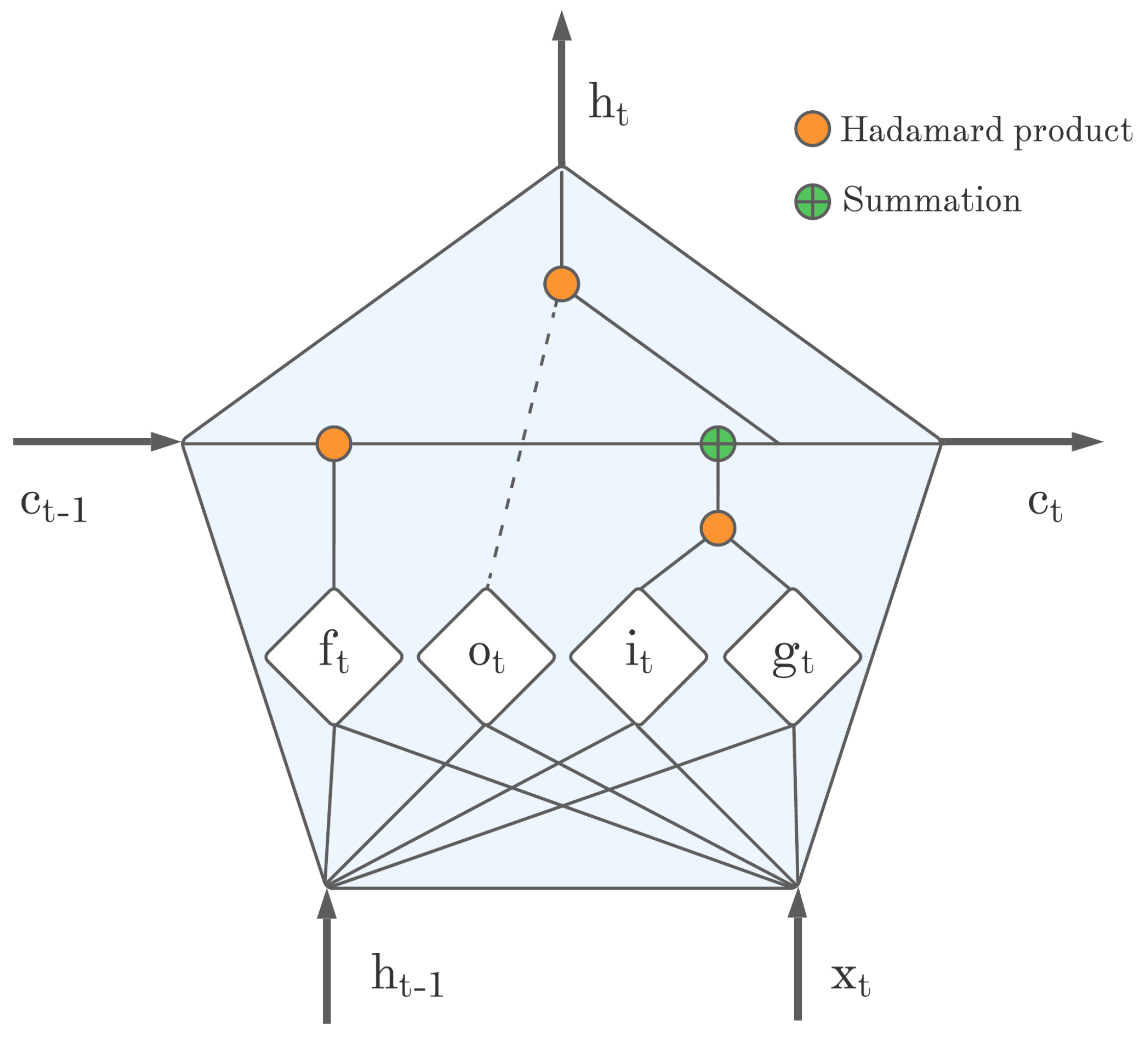
To reduce the time required to use the heat-flux sensor, this paper presents a way to predict the sensor output based on the same input data using deep learning. Deep learning is a subfield of machine learning in artificial intelligence that uses multiple layers of data processing operations [48]. In this research, long short-term memory (LSTM), a kind of recurrent neural network (RNN), was used. LSTMs as a subset of RNNs have cycles feeding the connected activation units [49,50,51], which carry information from layer to layer, including the information from the previous time step. The architecture of the LSTM unit is shown in Figure 2. The inclusion of the previous timestamp information in the decision of the LSTM unit is the reason why this kind of RNN architecture works well in time-series prediction or other regression problems for sequential data (e.g., natural-language processing), and, thus, is used in this research.
As shown in Figure 2, the LSTM unit has six operations [52], defined in a following way:
i t = σ W i i x t + b i i + W h i h t 1 + b h i ,
f t = σ W i f x t + b i f + W h f h t 1 + b h f ,
g t = t a n h W i g x t + b i g + W h g h t 1 + b h g ,
o t = σ W i o x t + b i o + W h o h t 1 + b i o ,
c t = f t c t 1 + i t g t ,
h t = o t t a n h c t ,
where x t is the input data in a time t, h t 1 and is an output from time t 1 . f t , i t , g t are forget gate, input gate, and cell gate, respectively, defined by the expressions (6). c t 1 is cell state from the time t 1 and c t is cell state for the current time t. o t is the output gate defined by the expression in (6), and, finally, h t is the hidden state (output of the LSTM unit) at time t. Analyzing Figure 2 and the expressions (6), it becomes clear why the LSTM architecture is well-suited for modeling sequential problems. The reason lies in the combination of the input of the current time t with the cell state and the hidden state from the previous time t 1 . Thus, the information for the new output is formed not only by applying neural network operations to the input data, but also by the information (relations) from the past.
If the model has more than one layer of stacked LSTM units, then the input x t i of the next layer i is a hidden state h t i 1 , which is an output of the previous layer. When we train a model defined in this way, the last hidden state h t n of the n-th layer is compared to the true value and a cost function is formed (usually a mean square error function). Then, backpropagation is used to adjust the model parameters so that the final output is as close as possible to the desired result. The cost function is minimized using a gradient descent optimization method with respect to the specified model parameters. In this research, we used Adam [53,54], an efficient stohastic optimization algorithm, for gradient descent optimization. The efficiency of the model performance can also be improved by dividing the training data into batches. In this way, we updated the model parameters several times in a training epoch so that less memory was consumed while the final result is not affected [55,56]. The biggest challenge in building a high-quality deep-learning model is avoiding overfitting. This is because deep learning has a large number of parameters that are backpropagated for the desired outcome, so it is possible for the model to perform well on training data but poorly on test data. Regularization techniques are used to generalize the model. The most common of these is the dropout, in which we neglect a strictly defined set of parameters at each parameter update. In this process, units are temporarily removed from the network, and the selection of units to be removed is random. Each unit has a fixed retention probability, p, independent of the other units. The main advantage of this method is the ease of implementation and improvement in model performance, while the main disadvantage is the increase in training time [57]. Two other regularization techniques are also used to overcome the overfitting problem: L1 and L2 regularization. They are defined as constraints implemented in the loss function. L1 regularization constraint uses the L1 norm that forces the model parameters to become zero, while L2 regularization uses the L2 norm that forces the model parameters towards zero [58,59,60]. In this way, we neglect the effects of data inputs that are far from the rest of the data in their environment.

2.4. Experimental Setup and Research Design

In order to implement the procedure based on deep learning, the first step in this research is to collect measurement data. Therefore, the in-situ measurement was performed according to the knowledge described in Section 2.2, i.e., following standard ISO 9869-1 [22]. The measurements were performed in a laboratory on wall specimens in true scale under laboratory environmental conditions on one side and simulated conditions on the other side. For the simulation, a climate chamber was used to simulate three types of conditions (winter, summer, and transitional, i.e., spring/fall). The climate chamber was equipped with an air conditioning unit that can simulate these conditions. All operations and program settings were defined with the PC operational unit placed alongside the chamber. Three types of walls were tested: specimen 1 (S1) was a concrete wall, specimen 2 (S2) was a concrete wall with mineral wool insulation facing the climate chamber, and specimen 3 (S3) was a concrete wall with extruded polystyrene (EPS) insulation facing the laboratory. The HFM sensors were placed on the laboratory side, as shown in Figure 3, and the measurement site was protected from the influence of sunlight entering through the windows. Table 2 shows information about each specimen with calculated thermal resistances and U-values according to ISO 6946 [30] based on thermal conductivity values derived from Croatian technical regulation [61].
The results of HFM measurement were analyzed using the average method defined by expression (4). Since the duration of the measurement must be at least 72 h, the deep-learning model was applied so that the training period did not exceed 72 h, to define the maximum period in which the HFM sensor must be used. After 72 h, the deep-learning model predicted the heat flux if the acceptance criteria from Table 1 were met. The HFM measurement was continued after 72 h to compare the resulting U-value from the HFM measurement ( U H F M ) with the U-value from the heat flux predicted by the deep-learning model ( U D L ). Both values were compared with the theoretical U-value according to ISO 6946 ( U I S O ) [30], so that the results of this research can be compared with related papers [23,27,33,45,46,47]. This research methodology is clearly presented in Figure 4.
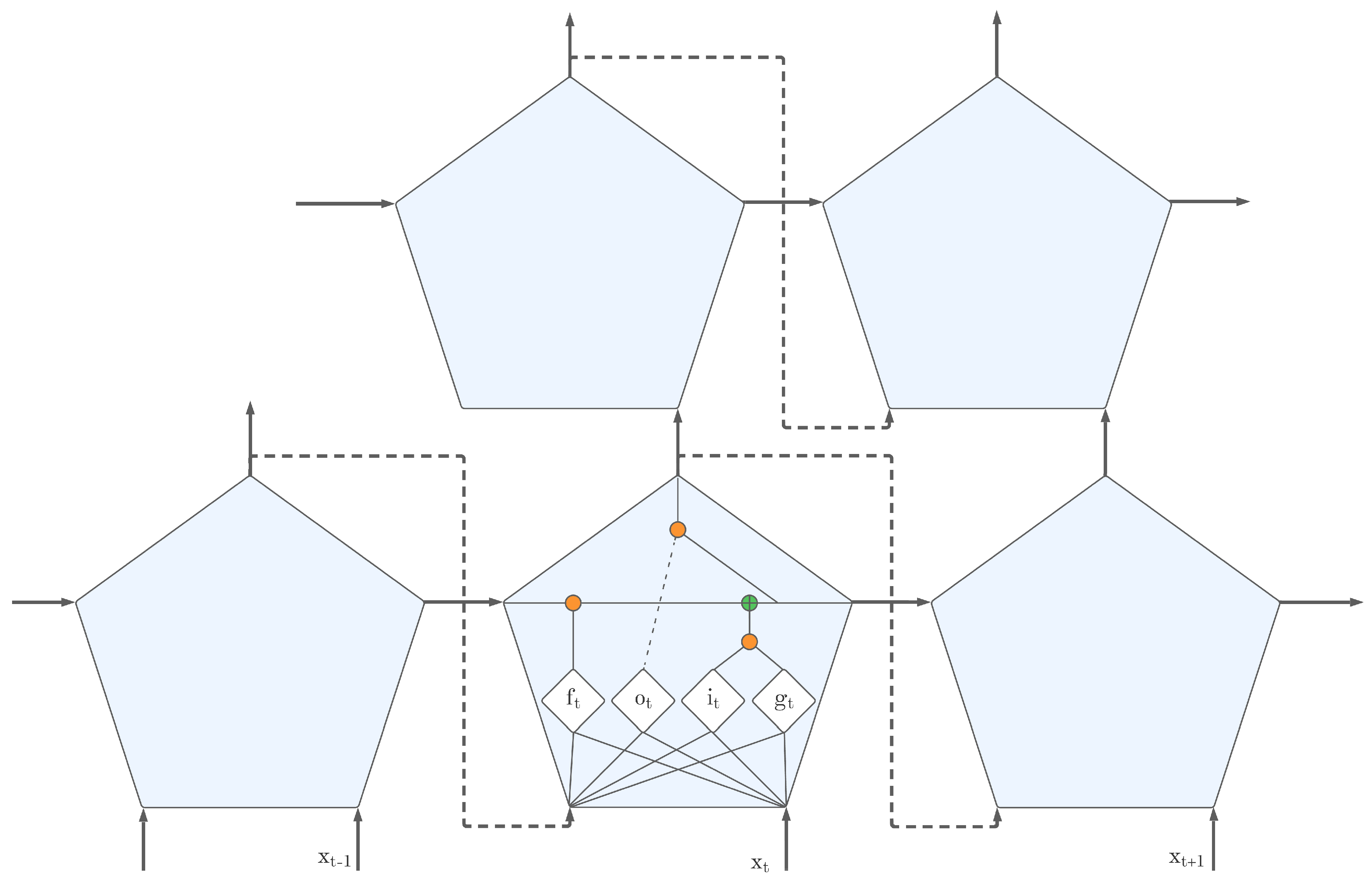
For each measurement, a deep-learning model was built based on the recurrent LSTM architecture. Each model consists of a fully connected multilayer set of LSTM units, where the final output is the desired outcome that is backpropagated by the loss function formed between this value and the heat-flux rate registered in the observed time step. The architectural scheme with more than one LSTM layer connected in a chain is shown in Figure 5. The model parameters were updated after a particular batch was passed. Regularization techniques were included with dropout and L2-regularization. The loss function used for backpropagation was the mean square error (MSE), while the root mean square error (RMSE) was used for the analysis of the prediction results because it is in the same units as the observed heat-flux rate, so the deviation between two time series across epochs is quite straightforward. In addition, the comparison between U D L and U H F M with U I S O was observed by the relative difference in dependance of U I S O at the end of the measurement as well as across the time series. Two acceptance limits were set (10%, which is characterized as very good prediction, and 20% which is characterized as good prediction). These limits were set in accordance with the literature, where we found that the authors were satisfied with the given results.
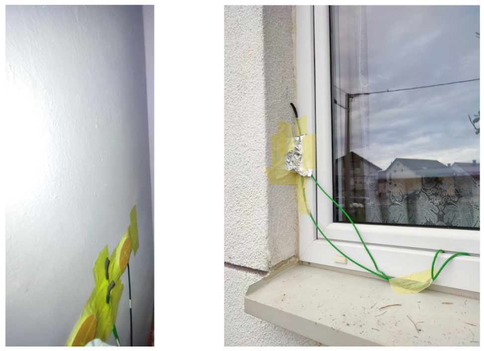
To investigate the applicability of the proposed method under in-situ conditions, we performed an HFM test on an exterior wall of a single-family house with unknown U-value. The measurement according to ISO 9869-1 [22] was performed in a period from 5th of November (12 h) to 16th of November (12 h) 2021. The measurement site was a house in the northern part of Croatia (municipality of Kotoriba) in autumn with an average temperature difference of 7.5 ° C between indoor and outdoor environment. The experimental setup can be seen in Figure 6 and the results are presented in Section 3.

3. Results

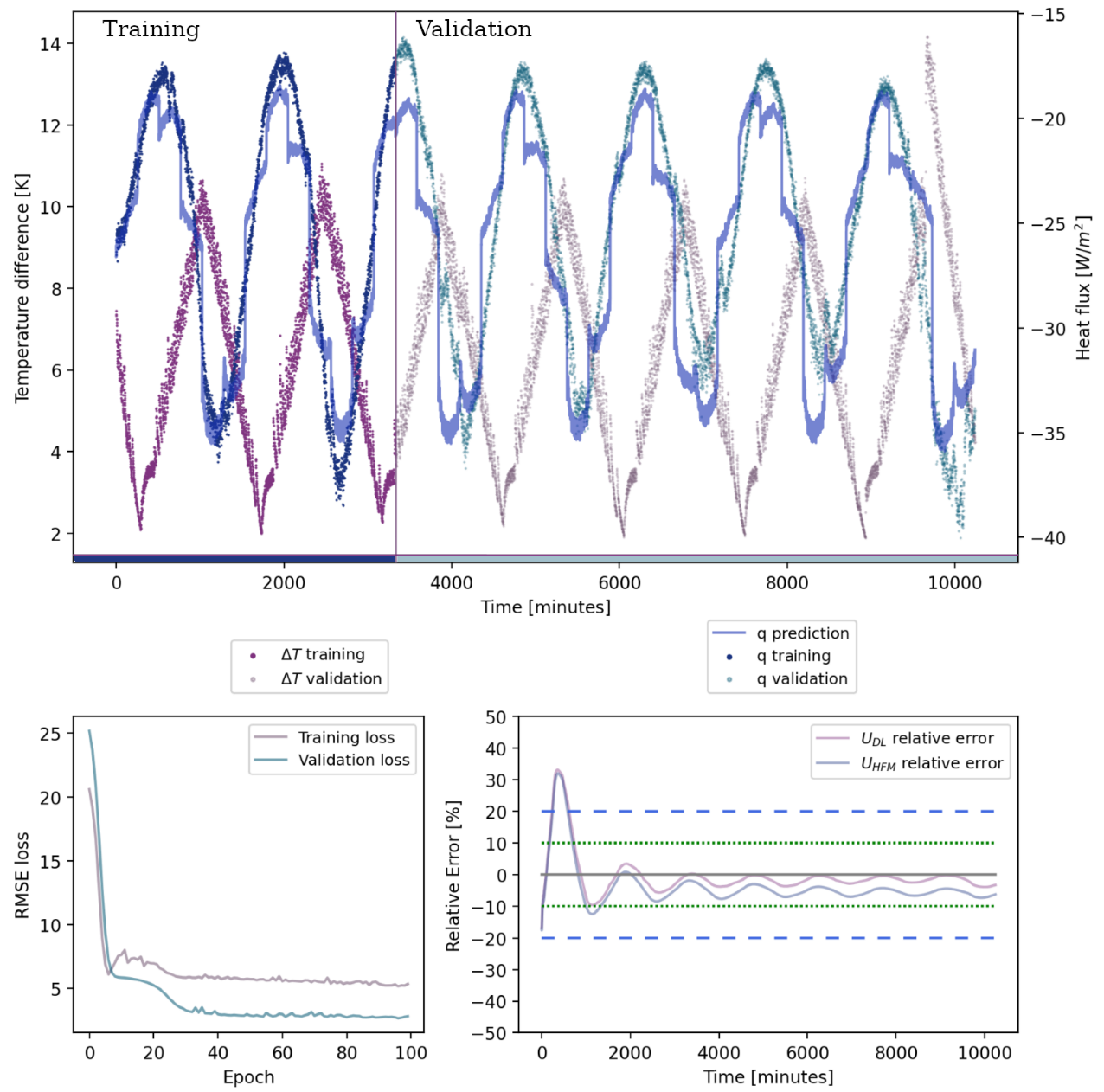
According to the methodology described in Section 2, an experimental research was conducted. The deep-learning method was applied after the results had been collected, according to ISO 9869-1. Predictions of HFM sensor results for three specimens under three conditions were observed. The predictions were made such that the developed deep-learning model performed the learning part of the first third of the collected results, while the performance of the model was determined by comparing two time series (predicted vs. measured) over the entire measurement period. Since the focus of interest was on the assessment of the in-situ U-value, an analysis was also performed for all experimental cases of U-value changes over a period of time, comparing the U-value from the predicted HFM time series ( U D L ) and the measured one ( U H F M ) with the U-value calculated according to ISO 6946 ( U I S O ). For each specimen type, the best solution from the three analyzed simulated conditions is presented: input time series, measured heat-flux rate, and heat-flux rate prediction in a graph, below which are two other graphs—one representing the learning rate and the other the described U-value comparison.
Specimen S1 is a 13.5 cm thick concrete wall with only one layer, as described in the Table 2 ( U I S O = 4.30 W/(m2K)). The deep-learning model chosen for the best conditions (winter) is an LSTM model with 16 LSTM layers. The time series were rearranged in batches of 256 points so that the model parameters were updated at the end of each batch rather than just at the end of the epoch in the training period. To avoid overfitting, two efficient regularization techniques were used: Dropout ( p = 0.5 ) and L2 regularization ( λ = 0.05 ). Figure 7 shows the performance of this model, where it can be seen that, after 100 epochs of training, the model predicts the HFM results such that it outperforms the HFM method when the U-value is calculated from these two time series and compared to the U I S O .
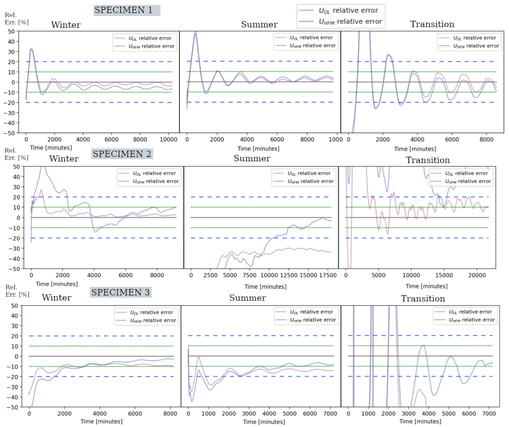
The other two specimens, S2 and S3, are insulated walls with the same U-value ( U I S O = 0.21 W/(m2K)) but different cross sections. The base for both is a 13.5 cm thick concrete wall. The insulation of S2 consists of 16 cm mineral wool facing the climatic chamber, while 16 cm EPS facing the laboratory was used for S3. Both specimens performed best in winter conditions in terms of the quality of the results. The selected LSTM deep-learning model is a model with 16 LSTM layers for S2 and a model with 8 LSTM units for S3. The time series were rearanged in batches of 128 points for S2 and 256 points for S3. Overfitting was again solved by dropout ( p = 0.5 for both cases) and L2 regularization ( λ = 0.01 for S2 and λ = 0.02 for S3). The model for S2, trained over 100 epochs (see Figure 8), again outperforms the HFM measurement result when considering the U-value. The final U-value not only has a lower relative error compared to U I S O , but also shows a more stable U-value solution over the entire measurement period. Although the model for S3 was trained over 300 epochs, it shows a worse solution than the model for S2, which has a stable solution with a relative error of about 10%, compared to U I S O . The reason for these more stable solutions is discussed in Section 4.
The parameters of all analyzed models are listed in the Table 3. They were chosen after fine tuning considering the listed parameters from Table 3, when a model achieved the best performance considering HFM prediction and U-value estimation from these results. The data and the open-source software solution can be found in the GitHub repository of one of the authors [62], so each model can be re-evaluated independently. The comparison of the U-values of all nine models is shown in Figure 9.
As can be seen in Figure 9 the most stable solution was recorded for the specimen with concrete wall. The reason for this is the relatively low thermal resistance (i.e., the high U-value), so the unfavorable conditions have little influence on the registered heat flux, resulting in a very stable time series of the U-value. The results for the winter and summer conditions are of high quality, while the results for the transition period are of low quality considering the stability conditions from ISO 9869-1. On the other hand, these results are very good when compared with our criteria defined in Section 2.4, based on the relevant literature sources from Section 1, because the deep-learning model result varied by 10% relative error around the U-value calculated by ISO 6946. This instability is the reason why we set the dropout parameter to be 0 (i.e., neglected) for models predicting results for the transition period. This parameter increased the instability of the prediction, so the registered results for models that included dropout were worse than the results that neglected this parameter. For all environmental conditions, the U-values calculated by deep-learning models outperformed the U-values from measured heat-flux rates. If we consider the specimen with the mineral wool facing climate chamber, a stable and high-quality result was registered only for the winter conditions. For the summer, we have a stable but low-quality result (stable between 30% and 40% relative error compared to U I S O ), and, for the transition period, we have a low-quality result compared to the ISO 9869-1 criteria, but also a relatively good result compared to the literature, as it varies around 10% relative error and does not exceed 20%. For the case where the EPS insulation faced the laboratory, representing interior insulation, the worst results were registered, both with respect to the stability criteria and compared to the literature. The HFM results are closer to the expected value than the deep-learning model results for all environmental conditions, while the deep-learning model results are more stable for winter and summer conditions.

Pilot In-Situ Measurement

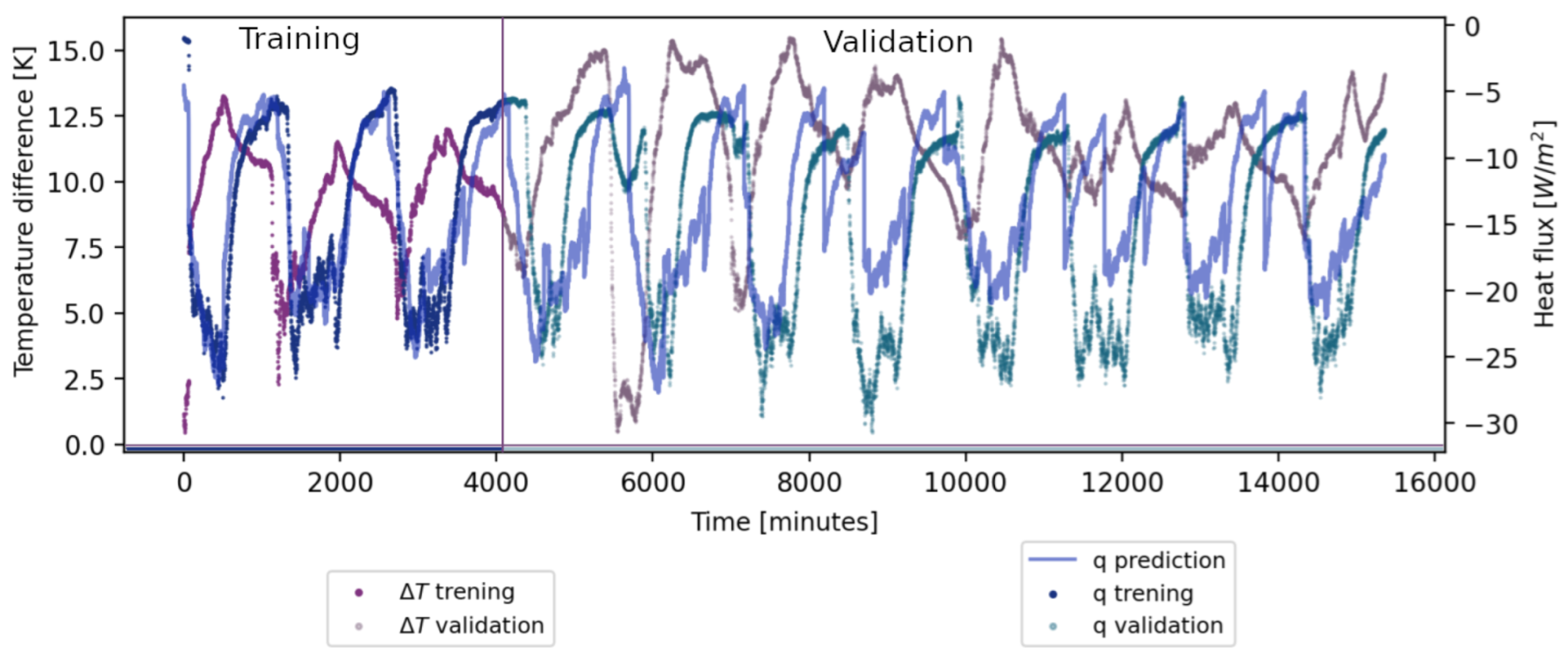
As defined in Section 2.4, one pilot in- situ measurement was performed. The outdoor temperature never exceeded the indoor temperature throughout the measurement, so, as can be seen in Figure 10, the heat flux did not change the orientation. The deep-learning model was created following the same methodology as for the laboratory experiments. The training period did not exceed the first 72 h and the deep-learning model consists of eight LSTM layers. The dataset was grouped into batches of 512 entries; the dropout probability parameter was 0.5, and the L2 regularization parameter was set to 0.05. The results showing the temperature difference with the measured and predicted heat fluxes can be found in Figure 10.
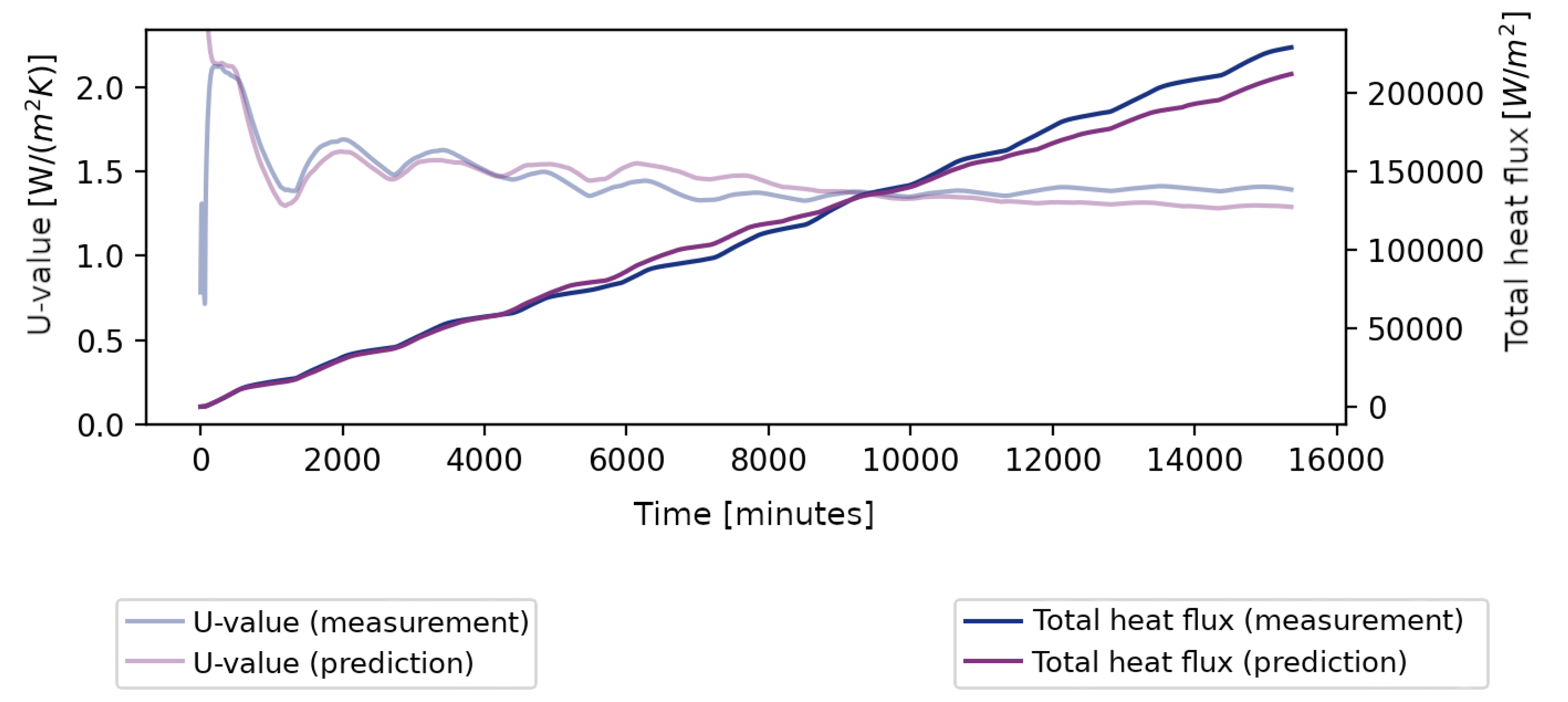
Since the U-value is unknown, we decided to show the comparison of U-value time series throughout the measurement period, as well as the comparison between the predicted total heat flux and the measured total heat flux that passed through the wall during the measurement period. As can be seen in Figure 11, the predicted results show promise for application under in-situ conditions. When U-values were calculated from measured and predicted heat fluxes according to the standard ISO 9869-1 as specified in Section 2.2, the registered difference between U H F M (1.4160 Wm 2 K 1 ) and U D L (1.1552 W 2 K 1 ) was 17.8%. Further research is needed to confirm these findings in different conditions. This research is ongoing and will be published elsewhere.

4. Discussion

As shown in Figure 9 and Table 3, nine different cases were analyzed as part of the research. Figure 9 shows the time series of the U-value when observed over the whole measurement period, which reveals the effects of the heat-flux rate change on the U-value, in a time. However, the criteria of ISO 9869-1 allow us to find any period of at least 72 h that meets the stability criteria (Table 1). For this reason, we discuss not only the results from Figure 7, Figure 8 and Figure 9, but also the U-values calculated from the measured and predicted time series where the stability criteria were maximized. For this reason, a new table was created showing the calculated U-values for all nine test cases (Table 4). Winter conditions are the most suitable for HFM measurement because heat flows from the laboratory to the climatic chamber. This is confirmed by the results (Figure 9), as we registered the most stable results in winter, which are also the most reliable for these climatic conditions. For the transitional period, the worst results were registered, which is logical because the temperature difference (as well as the heat flux) varied around zero for each sample, resulting in an unstable U-value time series, since the temperature difference is the second term of the calculation ratio. Under summer conditions, the samples performed similarly to winter conditions, since a similar temperature gradient was simulated.
In most test cases, we registered a more stable solution for the U-value calculated using the predicted heat-flux rate. The reason for this could be the use of regularization techniques in the training period, so that the model predicts the heat fluxes in such a way that it is immune to variations related to external influences (e.g., variations in indoor temperature). These influences are a particular problem for well-insulated walls, since the heat flux through a well-insulated wall is much lower than through a wall with a high U-value (i.e., with a low thermal resistance), so that sudden influences lead to sudden peaks that the HFM sensor registers. The described problem leads to a problem in meeting the stability criteria, which leads to an increase in the measurement time.
If we now consider the U-values calculated by the average method from ISO 9869-1 [22] for the best registered stability criteria, we can observe other important information. In this way, the results in Table 4 were developed—they are calculated by the average method in the period where the bast stability criteria from [22] are satisfied. When observing Table 4, it can be seen that the deep-learning models for winter conditions registered a relative error of less than 5% to the theoretical U-value for all three samples, which is a very important observation. For the U-value from measured heat fluxes, we found a deviation for S2. The reason for this is the effect of peaks (shown in the results plot in Figure 7) registered in the heat-flux time series. The results of U H F M were worse in summer than in winter, where deep learning U D L outperformed the U H F M calculated from the measured values. The transition period was again the worst when considering both U D L and U H F M determination, which is consistent with the literature. Very good results for the transition period were registered for the concrete wall and the EPS insulated wall only for the U H F M calculated from the measured heat fluxes. These results are good under laboratory conditions, but these environmental conditions are not reliable, so it is not advisable to perform in-situ measurements under such climatic conditions. As for the wall type, the most reliable results were registered for S1. The results are reliable because S1 has a low thermal resistance, so higher values of heat flux rates were registered and any unfavorable condition for the measurement has a lower influence on the final heat flux registered in a given time step.
When analyzing the in-situ pilot measurement, several differences from the laboratory experiments can be observed. The temperature difference and the measured heat flux have more complex behavior compared to the laboratory experiment, as does the predicted heat flux. Although the prediction of the heat flux seems to be worse than in some laboratory experiments, when we visually compare the predicted U-value with the measured value, we can see that there are relatively small differences between the two. Similar can be seen when observing the predicted and total heat flux. In addition, when we compare U H F M and U D L for this case, a relative difference in respect to U H F M falls within the limits of ± 20 % , so we can characterize this prediction result as good considering the characterization criteria defined in Section 2.4. This shows that the proposed method has the potential to be used under in-situ conditions, but it should be thoroughly analyzed to discover its full potential.

5. Conclusions

This paper investigated the possibility of using deep learning to reduce the time in which the HFM sensor must be used was investigated. It also investigates whether the developed deep-learning models are more resilient to unfavorable conditions. From nine analyzed test cases, it is found that deep learning is not only capable of replacing the HFM sensor when properly deployed, but also achieves acceptable, if not even better, results in most cases. Transition environmental conditions lead to unstable results, both considering HFM measurement and deep-learning prediction. As can be seen in the Table 4, there may be a time interval in the transition period where the stability criteria from ISO 9869-1 are met, but the results are generally very unstable, and it can not be concluded that every result collected in the transition period behaves similarly. The best results were observed for winter conditions, and acceptable ones for summer conditions. This is consistent with the literature, and the reason for this is the occurrence of a high thermal gradient. The most stable results were observed for high U-values, and the reason for this is the high heat flux through the tested specimen, so unpredictable events have little influence on the heat flux. For low U-values, this influence is not negligible, so the measured heat flux leads to an unstable U-value prediction if there is a large number of such events. DL prediction can solve this problem because the model generalizes the predicted result using regularization techniques applied in a training period; therefore, sudden changes in the measured heat flux are neglected in the prediction. This leads to a decrease in measurement time, since the stability criteria are met earlier when estimating the U-value using the predicted heat flux than using the measured one. This is the most important conclusion and can be clearly observed for the S2 specimen under winter conditions. In this test case, the measurement has three peaks, which have a great impact on the instability of the calculated U-value according to the average method from ISO 9869-1. If we consider the predicted heat flux, there are no peaks and, therefore, the time series of the calculated U-value is stable around the expected theoretical U-value. For unstable time series such as those in the transition period, methods based on reservoir computing specifically designed for unstable systems could probably be used ([63,64]), but this should be investigated further.
This research was conducted in a laboratory; therefore, in order to draw more accurate conclusions, further research needs to be conducted in situ under real climatic and real use conditions. Based on the results of in-situ measurements, the effects of stohastically determined real outdoor and indoor environmental conditions could be explored in detail. In order to explore the abovementioned, we conducted pilot in-situ measurements and predictions of the model that result in a relative difference of 17.8 % when we compare U D L to U H F M and encourage future research on this topic.

Author Contributions

Conceptualization, S.G., B.D.B. and M.G.; Data curation, S.G. and M.G.; Formal analysis, S.G.; Funding acquisition, S.G. and B.M.; Investigation, S.G., B.M. and B.D.B.; Methodology, S.G., B.M. and B.D.B.; Project administration, B.M.; Resources, B.M. and M.G.; Software, S.G.; Supervision, B.M. and B.D.B.; Validation, S.G., B.M. and M.G.; Visualization, S.G.; Writing—original draft, S.G.; Writing—review & editing, S.G., B.M., B.D.B. and M.G. All authors have read and agreed to the published version of the manuscript.

Funding

This research received no external funding.

Institutional Review Board Statement

Not applicable.

Informed Consent Statement

Not applicable.

Data Availability Statement

Not applicable.

Acknowledgments

We would like to acknowledge company Institut IGH d.d. for giving us the opportunity to conduct experimental research by using their laboratory equipment. One of the authors (S.G.) would like to acknowledge the Croatian Science Foundation and European Social Fund for the support under the project ESF DOK-01-2018.

Conflicts of Interest

The authors declare no conflict of interest.

References

  1. Commission, E. A Clean Planet for All—A European Strategic Long-Term Vision for A Prosperous, Modern, Competitive and Climate Neutral Economy; (COM (2018) 773 Final); European Commission: Brussels, Belgium, 2018. [Google Scholar]
  2. Buildings Performance Institute Europe (BPIE). State of the Building Stock Briefing; BPIE: Brussels, Belgium, 2017. [Google Scholar]
  3. Jensen, P.A.; Maslesa, E.; Berg, J.B.; Thuesen, C. 10 questions concerning sustainable building renovation. Build. Environ. 2018, 143, 130–137. [Google Scholar] [CrossRef]
  4. Laaroussi, Y.; Bahrar, M.; Zavrl, E.; Mankibi, M.E.; Stritih, U. New qualitative approach based on data analysis of European building stock and retrofit market. Sustain. Cities Soc. 2020, 63, 102452. [Google Scholar] [CrossRef]
  5. Kavgic, M.; Mavrogianni, A.; Mumovic, D.; Summerfield, A.; Stevanovic, Z.; Djurovic-Petrovic, M. A review of bottom-up building stock models for energy consumption in the residential sector. Build. Environ. 2010, 45, 1683–1697. [Google Scholar] [CrossRef]
  6. Nardi, I.; Lucchi, E.; de Rubeis, T.; Ambrosini, D. Quantification of heat energy losses through the building envelope: A state-of-the-art analysis with critical and comprehensive review on infrared thermography. Build. Environ. 2018, 146, 190–205. [Google Scholar] [CrossRef] [Green Version]
  7. Bazazzadeh, H.; Pilechiha, P.; Nadolny, A.; Mahdavinejad, M.; sara Hashemi safaei, S. The Impact Assessment of Climate Change on Building Energy Consumption in Poland. Energies 2021, 14, 4084. [Google Scholar] [CrossRef]
  8. Ji, Q.; Bi, Y.; Makvandi, M.; Deng, Q.; Zhou, X.; Li, C. Modelling Building Stock Energy Consumption at the Urban Level from an Empirical Study. Buildings 2022, 12, 385. [Google Scholar] [CrossRef]
  9. Yadav, M.; Agarwal, M. Biobased building materials for sustainable future: An overview. Mater. Today Proc. 2021, 43, 2895–2902. [Google Scholar] [CrossRef]
  10. Shawa, B.A. The ability of Building Stock Energy Models (BSEMs) to facilitate the sector’s climate change target in the face of socioeconomic uncertainties: A review. Energy Build. 2022, 254, 111634. [Google Scholar] [CrossRef]
  11. Li, X.; Yao, R. Modelling heating and cooling energy demand for building stock using a hybrid approach. Energy Build. 2021, 235, 110740. [Google Scholar] [CrossRef]
  12. Martín-Garín, A.; Millán-García, J.A.; Terés-Zubiaga, J.; Oregi, X.; Rodríguez-Vidal, I.; Baïri, A. Improving Energy Performance of Historic Buildings through Hygrothermal Assessment of the Envelope. Buildings 2021, 11, 410. [Google Scholar] [CrossRef]
  13. Buda, A.; de Place Hansen, E.J.; Rieser, A.; Giancola, E.; Pracchi, V.N.; Mauri, S.; Marincioni, V.; Gori, V.; Fouseki, K.; López, C.S.P.; et al. Conservation-Compatible Retrofit Solutions in Historic Buildings: An Integrated Approach. Sustainability 2021, 13, 2927. [Google Scholar] [CrossRef]
  14. Lizarraga, J.M.P.S.; Picallo-Perez, A. Design and optimization of the envelope and thermal installations of buildings. In Exergy Analysis and Thermoeconomics of Buildings; Elsevier: Amsterdam, The Netherlands, 2020; pp. 911–1005. [Google Scholar] [CrossRef]
  15. Thani, S.K.S.O.; Mohamad, N.H.N.; Idilfitri, S. Modification of Urban Temperature in Hot-Humid Climate Through Landscape Design Approach: A Review. Procedia-Soc. Behav. Sci. 2012, 68, 439–450. [Google Scholar] [CrossRef] [Green Version]
  16. Milovanović, B.; Bagarić, M. How to achieve Nearly zero-energy buildings standard. J. Croat. Assoc. Civ. Eng. 2020, 72, 703–720. [Google Scholar] [CrossRef]
  17. Gaši, M.; Milovanović, B.; Gumbarević, S. Comparison of Infrared Thermography and Heat Flux Method for Dynamic Thermal Transmittance Determination. Buildings 2019, 9, 132. [Google Scholar] [CrossRef] [Green Version]
  18. Gomes, M.G.; Flores-Colen, I.; Manga, L.; Soares, A.; de Brito, J. The influence of moisture content on the thermal conductivity of external thermal mortars. Constr. Build. Mater. 2017, 135, 279–286. [Google Scholar] [CrossRef]
  19. Lucchi, E. Thermal transmittance of historical brick masonries: A comparison among standard data, analytical calculation procedures, and in situ heat flow meter measurements. Energy Build. 2017, 134, 171–184. [Google Scholar] [CrossRef]
  20. Bienvenido-Huertas, D.; Moyano, J.; Marín, D.; Fresco-Contreras, R. Review of in situ methods for assessing the thermal transmittance of walls. Renew. Sustain. Energy Rev. 2019, 102, 356–371. [Google Scholar] [CrossRef]
  21. Martin, M.; Chong, A.; Biljecki, F.; Miller, C. Infrared thermography in the built environment: A multi-scale review. Renew. Sustain. Energy Rev. 2022, 165, 112540. [Google Scholar] [CrossRef]
  22. ISO 9869-1:2014; Thermal Insulation—Building Elements—In-Situ Measurement of Thermal Resistance and Thermal Transmittance—Part 1: Heat Flow Meter Method. International Organization for Standardization (ISO): Geneva, Switzerland, 2014.
  23. Evangelisti, L.; Scorza, A.; Vollaro, R.D.L.; Sciuto, S.A. Comparison between Heat Flow Meter (HFM) and Thermometric (THM) Method for Building Wall Thermal Characterization: Latest Advances and Critical Review. Sustainability 2022, 14, 693. [Google Scholar] [CrossRef]
  24. Bienvenido-Huertas, D. Assessing the Environmental Impact of Thermal Transmittance Tests Performed in Façades of Existing Buildings: The Case of Spain. Sustainability 2020, 12, 6247. [Google Scholar] [CrossRef]
  25. Tejedor, B.; Gaspar, K.; Casals, M.; Gangolells, M. Analysis of the Applicability of Non-Destructive Techniques to Determine In Situ Thermal Transmittance in Passive House Façades. Appl. Sci. 2020, 10, 8337. [Google Scholar] [CrossRef]
  26. Trabelsi, A.; Belarbi, R.; Abahri, K.; Qin, M. Assessment of temperature gradient effects on moisture transfer through thermogradient coefficient. Build. Simul. 2012, 5, 107–115. [Google Scholar] [CrossRef]
  27. Nardi, I.; Ambrosini, D.; de Rubeis, T.; Sfarra, S.; Perilli, S.; Pasqualoni, G. A comparison between thermographic and flow-meter methods for the evaluation of thermal transmittance of different wall constructions. J. Phys. Conf. Ser. 2015, 655, 012007. [Google Scholar] [CrossRef] [Green Version]
  28. Evangelisti, L.; Guattari, C.; Asdrubali, F. Comparison between heat-flow meter and Air-Surface Temperature Ratio techniques for assembled panels thermal characterization. Energy Build. 2019, 203, 109441. [Google Scholar] [CrossRef]
  29. Rezvani, F.; Bribián, I.Z. Evaluating in-situ thermal transmittance measurement to analyze devia-tions between actual house thermal performance and modelled one by means of energy simulation software. Rev. Constr. 2019, 18, 311–322. [Google Scholar] [CrossRef]
  30. ISO 6946:2017; Building Components and Building Elements—Thermal Resistance and Thermal Transmittance—Calculation Methods. International Organization for Standardization (ISO): Geneva, Switzerland, 2017.
  31. Roque, E.; Vicente, R.; Almeida, R.M.; da Silva, J.M.; Ferreira, A.V. Thermal characterisation of traditional wall solution of built heritage using the simple hot box-heat flow meter method: In situ measurements and numerical simulation. Appl. Therm. Eng. 2020, 169, 114935. [Google Scholar] [CrossRef]
  32. Meng, X.; Luo, T.; Gao, Y.; Zhang, L.; Shen, Q.; Long, E. A new simple method to measure wall thermal transmittance in situ and its adaptability analysis. Appl. Therm. Eng. 2017, 122, 747–757. [Google Scholar] [CrossRef]
  33. Gaspar, K.; Casals, M.; Gangolells, M. In situ measurement of façades with a low U-value: Avoiding deviations. Energy Build. 2018, 170, 61–73. [Google Scholar] [CrossRef]
  34. Marquez, J.M.A.; Bohorquez, M.A.M.M.S.G. A New Metre for Cheap, Quick, Reliable and Simple Thermal Transmittance (U-Value) Measurements in Buildings. Sensors 2017, 17, 2017. [Google Scholar] [CrossRef] [Green Version]
  35. Bienvenido-Huertas, D.; Moyano, J.; Rodríguez-Jiménez, C.E.; Marín, D. Applying an artificial neural network to assess thermal transmittance in walls by means of the thermometric method. Appl. Energy 2019, 233–234, 1–14. [Google Scholar] [CrossRef]
  36. Bienvenido-Huertas, D.; Rubio-Bellido, C.; Pérez-Ordóñez, J.L.; Moyano, J. Optimizing the evaluation of thermal transmittance with the thermometric method using multilayer perceptrons. Energy Build. 2019, 198, 395–411. [Google Scholar] [CrossRef]
  37. Gumbarević, S.; Milovanović, B.; Gaši, M.; Bagarić, M. Application of Multilayer Perceptron Method on Heat Flow Meter Results for Reducing the Measurement Time. Eng. Proc. 2020, 2, 29. [Google Scholar] [CrossRef]
  38. Gumbarević, S.; Milovanović, B.; Gaši, M.; Bagarić, M. Thermal transmittance prediction based on the application of artificial neural networks on heat flux method results. J. Phys. Conf. Ser. 2021, 2069, 012152. [Google Scholar] [CrossRef]
  39. Chen, L.; Zhan, C.; Li, G.; Zhang, A. An artificial neural network identification method for thermal resistance of exterior walls of buildings based on numerical experiments. Build. Simul. 2019, 12, 425–440. [Google Scholar] [CrossRef]
  40. Jordan, M.I.; Mitchell, T.M. Machine learning: Trends, perspectives, and prospects. Science 2015, 349, 255–260. [Google Scholar] [CrossRef]
  41. Linardatos, P.; Papastefanopoulos, V.; Kotsiantis, S. Explainable AI: A Review of Machine Learning Interpretability Methods. Entropy 2020, 23, 18. [Google Scholar] [CrossRef] [PubMed]
  42. Namuduri, S.; Narayanan, B.N.; Davuluru, V.S.P.; Burton, L.; Bhansali, S. Review—Deep Learning Methods for Sensor Based Predictive Maintenance and Future Perspectives for Electrochemical Sensors. J. Electrochem. Soc. 2020, 167, 037552. [Google Scholar] [CrossRef]
  43. Thomas, L.; Marino, B.; Muñoz, N. Steady-state and time-dependent heat fluxes through building envelope walls: A quantitative analysis to determine their relative significance all year round. J. Build. Eng. 2020, 29, 101122. [Google Scholar] [CrossRef]
  44. Gumbarević, S.; Dunović, I.B.; Milovanović, B.; Gaši, M. Method for Building Information Modeling Supported Project Control of Nearly Zero-Energy Building Delivery. Energies 2020, 13, 5519. [Google Scholar] [CrossRef]
  45. Gaspar, K.; Casals, M.; Gangolells, M. Influence of HFM Thermal Contact on the Accuracy of In Situ Measurements of Façades’ U-Value in Operational Stage. Appl. Sci. 2021, 11, 979. [Google Scholar] [CrossRef]
  46. Bienvenido-Huertas, D.; Rubio-Bellido, C.; Pérez-Ordóñez, J.L.; Oliveira, M.J. Automation and optimization of in-situ assessment of wall thermal transmittance using a Random Forest algorithm. Build. Environ. 2020, 168, 106479. [Google Scholar] [CrossRef]
  47. Asdrubali, F.; D’Alessandro, F.; Baldinelli, G.; Bianchi, F. Evaluating in situ thermal transmittance of green buildings masonries—A case study. Case Stud. Constr. Mater. 2014, 1, 53–59. [Google Scholar] [CrossRef]
  48. LeCun, Y.; Bengio, Y.; Hinton, G. Deep learning. Nature 2015, 521, 436–444. [Google Scholar] [CrossRef] [PubMed]
  49. Sak, H.; Senior, A.; Beaufays, F. Long Short-Term Memory Based Recurrent Neural Network Architectures for Large Vocabulary Speech Recognition. arXiv 2014, arXiv:1402.1128. [Google Scholar]
  50. Zia, T.; Zahid, U. Long short-term memory recurrent neural network architectures for Urdu acoustic modeling. Int. J. Speech Technol. 2018, 22, 21–30. [Google Scholar] [CrossRef]
  51. Greff, K.; Srivastava, R.K.; Koutnik, J.; Steunebrink, B.R.; Schmidhuber, J. LSTM: A Search Space Odyssey. IEEE Trans. Neural Netw. Learn. Syst. 2017, 28, 2222–2232. [Google Scholar] [CrossRef] [Green Version]
  52. Paszke, A.; Gross, S.; Massa, F.; Lerer, A.; Bradbury, J.; Chanan, G.; Killeen, T.; Lin, Z.; Gimelshein, N.; Antiga, L.; et al. PyTorch: An Imperative Style, High-Performance Deep Learning Library. arXiv 2019, arXiv:1912.01703. [Google Scholar]
  53. Kingma, D.P.; Ba, J. Adam: A Method for Stochastic Optimization. arXiv 2014, arXiv:1412.6980. [Google Scholar]
  54. Ruder, S. An overview of gradient descent optimization algorithms. arXiv 2016, arXiv:1609.04747. [Google Scholar]
  55. Smith, S.L.; Kindermans, P.J.; Le, Q.V. Don’t Decay the Learning Rate, Increase the Batch Size. arXiv 2017, arXiv:1711.00489. [Google Scholar]
  56. Hoffer, E.; Hubara, I.; Soudry, D. Train Longer, Generalize Better: Closing the Generalization Gap in Large Batch Training of Neural Networks. In Proceedings of the 31st International Conference on Neural Information Processing Systems, Long Beach, CA, USA, 4–9 December 2017; Curran Associates Inc.: Red Hook, NY, USA, 2017. NIPS’17. pp. 1729–1739. [Google Scholar]
  57. Srivastava, N.; Hinton, G.; Krizhevsky, A.; Sutskever, I.; Salakhutdinov, R. Dropout: A Simple Way to Prevent Neural Networks from Overfitting. J. Mach. Learn. Res. 2014, 15, 1929–1958. [Google Scholar]
  58. Alizadeh, S.; Fazel, A. Convolutional Neural Networks for Facial Expression Recognition. arXiv 2017, arXiv:cs.CV/1704.06756. [Google Scholar]
  59. Zeng, S.; Zhang, B.; Zhang, Y.; Gou, J. Collaboratively Weighting Deep and Classic Representation via l2 Regularization for Image Classification. In Proceedings of the 10th Asian Conference on Machine Learning, Beijing, China, 14–16 November 2018; Volume 95, pp. 502–517. [Google Scholar]
  60. Cobbe, K.; Klimov, O.; Hesse, C.; Kim, T.; Schulman, J. Quantifying Generalization in Reinforcement Learning. In Proceedings of the 36th International Conference on Machine Learning, Long Beach, CA, USA, 10–15 June 2019; Volume 97, pp. 1282–1289. [Google Scholar]
  61. Republic of Croatia Ministry of Construction and Physical Planning. Technical Regulation on Rational Use of Energy and Heat Retention in Buildings; Republic of Croatia Ministry of Construction and Physical Planning: Zagreb, Croatia, 2015.
  62. Gumbarević, S. 2022. Available online: https://github.com/sanjin94/HFMpred (accessed on 10 May 2022).
  63. Chattopadhyay, A.; Hassanzadeh, P.; Subramanian, D. Data-driven prediction of a multi-scale Lorenz 96 chaotic system using deep learning methods: Reservoir computing, ANN, and RNN-LSTM. Nonlin. Processes Geophys. 2020, 27, 373–389. [Google Scholar] [CrossRef]
  64. Martinuzzi, F.; Rackauckas, C.; Abdelrehim, A.; Mahecha, M.D.; Mora, K. ReservoirComputing.jl: An Efficient and Modular Library for Reservoir Computing Models. arXiv 2022, arXiv:2204.05117. [Google Scholar]
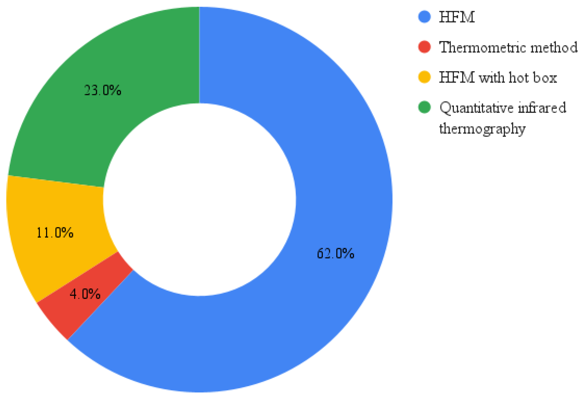
Figure 1. Distribution of research articles for each defined in-situ method for U-value determination according to [23].
Energies 15 05029 g001
Figure 2. Schematic view of the long short-term memory unit.
Energies 15 05029 g002
Figure 3. Schematic view of the experimental facility on the (left) and experimental setup on the (right).
Energies 15 05029 g003
Figure 4. Research methodology.
Energies 15 05029 g004
Figure 5. LSTM architecture when there is more than one layer.
Energies 15 05029 g005
Figure 6. Experimental setup for the pilot in-situ measurement.
Energies 15 05029 g006
Figure 7. Results for the deep-learning model developed for S1 under winter conditions.
Energies 15 05029 g007
Figure 8. Results for the deep-learning model developed for S2 under winter conditions.
Energies 15 05029 g008
Figure 9. U-value relative error throughout the measurement compared to the ISO 6946 U-value (predicted vs. measured results).
Energies 15 05029 g009
Figure 10. Results for the deep-learning model developed for the pilot in-situ measurement.
Energies 15 05029 g010
Figure 11. U-value and total heat flux comparison calculated on measured and predicted values for pilot in-situ measurement.
Energies 15 05029 g011
Table 1. Acceptance criteria defined by standard ISO 9869-1 [22] for ensuring the U-value converges to an asymptotical value.
Test DurationEnd vs. (End—24 h)First 2/3 vs. Last 2/3
min 72 h≤5%≤5%
Table 2. Specimen description and thermal characteristics.
SpecimenLayerLayers
Thickness [m]
λ
[W/(m K)] [61]
R T [m2 K/W] [30]U [W/(m2 K)] [30]
S1concrete0.1352.00.254.30
concrete0.1352.0
S2mineral wool0.160.0354.820.21
EPS0.160.035
S3concrete0.1352.04.820.21
Table 3. Analyzed deep-learning models.
ModelNumber of LayersBatch SizeDropout ProbabilityL2 Regularization ParameterNumber of Epochs
S1 winter162560.50.05100
S1 summer45120.050.01200
S1 transition412800.180
S2 winter161280.50.01100
S2 summer165120.50.00860
S2 transition161280.50.1150
S3 winter82560.10.02300
S3 summer85120.50.02200
S3 transition825600.005100
Table 4. Comparison of U-values calculated by the average method from the ISO 9869-1 applied on measured and predicted heat fluxes.
Specimen U ISO
[W/(m2K)]
U HFM
[W/(m2K)]
U DL
[W/(m2K)]
dU HFM [%] dU DL [%]
S1 winter4.304.064.16 5.58 3.26
S1 summer4.644.187.91−2.79
S1 transition3.883.769.77−12.56
S2 winter0.210.170.22−19.054.76
S2 summer0.280.1533.33 28 . 57
S2 transition0.410.33 (0.24) 195.2357.14 (14.29)
S3 winter0.210.210.200.00−4.76
S3 summer0.200.184.76−14.29
S3 transition0.190.089.52−61.90
1 Result in parenthesis is for the best stability criteria for measurement. It is not the best stability criteria for prediction, but it satisfies ISO 9869-1 criteria. Note: underlined values are those with relative error lower than 10%, which is characterized as very good.
Publisher’s Note: MDPI stays neutral with regard to jurisdictional claims in published maps and institutional affiliations.