Abstract
Transverse vibration of drillpipe in coring drilling is undesirable. Here, the influence of the core on drillpipe vibration is considered for the first time. Attention is focused on the vibrations of the coring drillpipe as these vibrations lead to contact and collision between drillpipe and core. A reduced-order model of drill string motion is established considering fluid load and core constraints. This model considers fluid action as distributed load and drillpipe as beam structure. The constraint of the core on lateral vibration of the drillpipe is simplified as a nonlinear force. The method of multiple scales is used to analyze the disturbance of the drillpipe’s primary resonance and harmonic resonance, and the influence law of different parameters on the drillpipe resonance is obtained. The results show that damping inhibits resonance vibration, and external excitation determines the resonance type. The existence of the core will aggravate the resonance vibration of the drillpipe. The analysis results are helpful in understanding the resonance of the drillpipe in coring drilling. Some measures to suppress resonance are given in this paper. This study can provide guidance for further research on drillpipe resonance in core drilling.
1. Introduction
Nowadays, exploring and developing various energy sources is still critical and a hot topic [1]. Core drilling is one of the most effective means of obtaining formation data for recognizing and evaluating reservoirs. In Figure 1, the principle of coring drilling is explained. The bottom hole assembly rotates to obtain the core and takes it to the ground. The drillpipe transmits pressure, impact, and rotary torque to the bottom hole. The working state of the coring bit depends on the performance of the drillpipe and formation factors. The complex borehole working environment will strongly impact the slender drill string. These complex working environments include but are not limited to high temperature and high-pressure working environments, the influence of mud drilling fluid flushing the bottom hole on the drillpipe, the interaction between bottom hole formation and the drill bit, and the collision between drillpipe string and the borehole wall, etc. These effects can cause the drillpipe to vibrate violently underground and often lead to the failure of the drillpipe. The failure of the drillpipe will damage the safety and economy of drilling work [2].
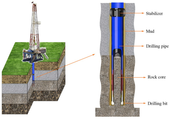
Figure 1.
Schematic diagram of core drilling.
Today, although vibration is used for drilling in many projects, we need to avoid harmful vibrations underground. Many scholars have studied the vibration of drillpipes. The longitudinal vibration, torsional vibration, and transverse vibration of the drillpipe were studied by Nikolaos. The results show that the transverse vibration of the drillpipe is the most serious [3]. Ritto established the nonlinear dynamic model of the drillpipe and analyzed the contact problem between the drillpipe and borehole wall [4]. Apostal, Haduch, and Williams [5] examined the lateral vibrations of a drillpipe by employing the finite element method. They also considered damping during failure analysis based on frequency responses. Jansen [6] modeled the drillpipe model and considered the effects of drilling fluid, stabilizer clearance, and stabilizer friction. Vaz and Patel [7] carried out an investigation into drillpipe dynamic stability and static deflection. Transverse vibrations were considered in this work. Following prior studies, Khulief and Al-Naser [8] conducted finite element analysis to include the BHA and drillpipe sections. Omojuwa E [9] studied the lateral vibration of BHA and analyzed the influence of drilling parameters on drillpipe failure. In recent work, Zhao [10] studied the resonance problem in coring drilling and believed that the contact between the drillpipe and rock stratum was nonlinear. Liang [11] simplified the composite coring drillpipe into a fully elastic beam structure and studied the lateral vibration of the drillpipe under different drilling pressures and speeds. Liu [12] considered the nonlinear vibration of the drillpipe affected by stabilizers and drilling fluid and discussed the stability of solutions and sensitivity to parameters. Kamgue Lenwoue, and Arnaud Regis′s study [13] on the lateral vibration of drillpipes found that the lateral vibration of drillpipes can also affect the stability of wellbore.
The complex bore-hole environment leads to complex and changeable vibration of the drillpipe. The actual vibration of the drillpipe is usually the coupling of transverse, torsional, and longitudinal vibrations. Compared to comprehensive drilling, core drilling has a small annular gap and high rotation speed. The transverse vibration of the drill string is more intense, and excessive transverse vibration will collide with the core. The core becomes a constraint on the transverse vibration of the drillpipe. This is also a feature of core drilling. In this work, the authors mainly focus on constructing analytical approximations for a better understanding of nonlinear behavior of drillpipes subjected to fluid forces. Compared to previous studies, the drillpipe is simplified as a simply supported beam structure at both ends. This is the first time that the core has been introduced as the constraint of transverse vibration of drillpipes and simplified as a cubic nonlinear spring force. On this basis, the motion control equation of drillpipe lateral vibration is established, and the motion equation is discretized into an ordinary differential equation using the Galerkin method. The corresponding equation of frequency amplitude is obtained through the method of multiple scales, and the influence of different parameters on resonance is analyzed.
2. Model Development
2.1. Simplified Model
As shown on the right of Figure 1, the drillpipe between the bit and the nearest stabilizer is selected as the research object. Bits and stabilizers are seen as hinged joints. The influence of drill mud is acting throughout the length of the beam. The force form can be simplified as a harmonic distributed force with an amplitude of (N/m). The damping force associated with the fluid around the drillpipe is also considered. This force has the form . The direction of the force is opposite to the speed of lateral movement of the drillpipe, where is the viscous damping coefficient (Ns/m2).
We can write the governing equation of motion based on the Bernoulli–Euler beam theory and the depiction shown in Figure 2.
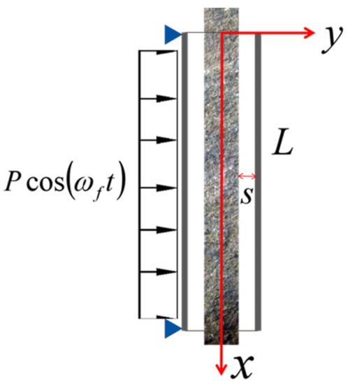

Figure 2.
Mechanical model of coring drillpipe under fluid action.
Figure 2.
Mechanical model of coring drillpipe under fluid action.
Here, is the transverse vibration displacement of the drillpipe, is the spatial coordinates along the drillpipe axis, is time coordinate, is the bending stiffness of the drillpipe, is the density of the drillpipe, is the cross-sectional area of the drillpipe, is the impact force between the inner wall of the drillpipe and core.
Transverse vibration and buckling deformation of the drillpipe in the complex underground environment can lead to contact collision between the drillpipe and core. As shown in Figure 3, it shows the equilibrium state of the drillpipe, distributed constraints, and two possible collision situations.
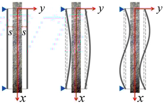
Figure 3.
Several forms of contact between coring drillpipe and core.
Here, is the nonlinear collision constraint force acting on the drillpipe along the pipe axis.
where is the distance between the inside of the drillpipe and the core, is the third-order nonlinear stiffness coefficient. The force model is in good agreement with the characteristic curve of the constraint force measured by the Paidoussis experiment, so it is widely used to simulate the collision between structures [14]. The qualitative characteristic curve of collision force is shown in Figure 4. When the transverse vibration is less than the distance between the drillpipe and the core, it indicates that there is no contact constraint force and no contact between the drillpipe and the core. On the contrary, collision constraints are generated.
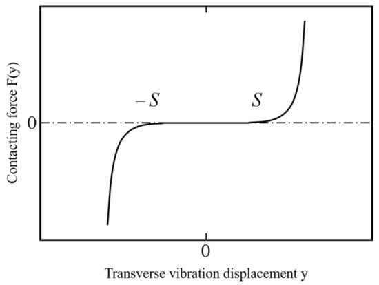
Figure 4.
The relationship between collision force and distance between drillpipe and core.
2.2. Governing Equations
Making the study universal, the following dimensionless parameters are introduced.
,,,,,,,.
The dimensionless equations of motion can be obtained as follows
The dimensionless collision binding force between drillpipe and core is as follows
For convenience, formula (3) can be simplified as follows
Here, the overdot () denotes the derivative with respect to the dimensionless time , while the prime () represents the derivative with respect to the dimensionless spatial variable . The boundary conditions can be obtained as
2.3. Discretization, Linear System, and Nonlinear Systems
The Galerkin technique simplifies the governing partial differential equation as a set of ordinary differential equations. The solution is assumed to be in the following form.
where is the nth-order vibration mode function and is the corresponding generalized coordinate. Substituting Equation (7) into Equation (5), multiplying by the trial function and integrating from 0 to 1, a nonlinear ordinary differential equations in matrix form can be obtained
where ,, represent the displacement, velocity and acceleration column vectors of the drillpipe after discretization, respectively., , , , represent the mass matrix, damping matrix, stiffness matrix, nonlinear collision force, and mud column vector of discrete systems, respectively. The following formulas can calculate the elements of these matrices and vectors.
In fact, any vibration beam’s eigen functions, also called mode shape functions, can be inherited from the base beam mode. For this paper, the trial function of the hinged beam at both ends can be selected as , and by substituting into Equation (8), then introducing as a dimensionless excitation frequency, Equation (8) is converted to the following form
where
3. Perturbation Solution for Response
For governing an equation with a cubic nonlinearity term and small excitation amplitude, the standard multiple scales method is used to obtain the approximate solution. Based on this method, the solution for the response can be written as
Therefore, the following can be obtained:
In addition, the derivative operator () is introduced, which results in different derivatives as
the derivative operator is also applicable to the calculation of the second derivative .
3.1. Primary Resonance
Considering weak damping and a small excitation term, Equation (14) can alternatively be written as
For the primary resonance, the excitation frequency approaches the system’s natural frequency. Here, the dimensionless excitation frequency is expressed as
where is the detuning parameter. In this paper, two time dimensions are solved as
After substituting Equations (25)–(27) into (24) and casting out the multiple terms of we can obtain
using Euler′s formula, we can obtain
We yield by multiplying the coefficients of each order from 0 to 1.
The solution of the second-order ordinary differential Equation (30) can be expressed as
Here, in which and are natural functions of , is the complex conjugate of . Substituting Equation (32) into Equation (31) we can obtain
where indicates the complex conjugate. Now, one can separate the secular term from Equation (34) and let the sum of the secular term′s coefficient equal zero.
Multiplying the to Equation (35) and substituting Equation (33) into Equation (35) with rearrangement results in
Introducing into Equation (36) and converting Equation (36) into trigonometric form, and separating the result into real and imaginary parts, one can obtain the modulation equations.
When and tend toward zero, Equation (37) reflects the steady-state response of the system.
3.2. Secondary Resonances
This section will focus on finding the secondary resonances that can occur in the system. Firstly, Equation (24) will be converted into the following form
After substituting Equations (26–67) into (38) and casting out the multiple terms of we can obtain
Extracting the coefficients of each order of from 0 to 1 yield.
The solution of the second-order ordinary differential Equation (40) can be expressed as
where contains the amplitudes and phases information and is the complex conjugate of . When putting Equation (42) into (41), it results
Equation (44) can be used to determine the form of secondary resonance based on different , which determines whether the secular term appears or not. Judging from the right part of Equation (44), one can obtain that the system will occur as a third order subharmonic and third order superharmonic resonances. The detailed description of subharmonic and superharmonic resonances are as follows.
3.2.1. Subharmonic Resonance
Based on the aforementioned analysis and introducing the detuning parameter , when the third order subharmonic resonances occur in the system, the dimensionless excitation frequency is expressed as
Substituting Equation (45) into (44) and separating the secular term
Similar to Equation (33), can be expressed as
Substituting into Equation (46) and multiplying the , with rearrangement, results in
Introducing into Equation (47) and converting Equation (47) into trigonometric form, and separating the result into real and imaginary parts, one can obtain the modulation equations.
When and tend toward zero, Equation (49) reflects the steady-state response of the system.
3.2.2. Superharmonic Resonance
When the third order superharmonic resonances occur in the system, the dimensionless excitation frequency is expressed as
Just like solving the third order subharmonic resonances problem, the secular term is derived as
Similarity, substituting and resetting, and separating the real and imaginary parts of Equation (51), we obtain
4. Amplitude-Frequency Response Analysis
4.1. Principal Resonance Response
To investigate the influence of different factors on the principal resonance response of the drillpipe, when , we selected different parameters for analysis.
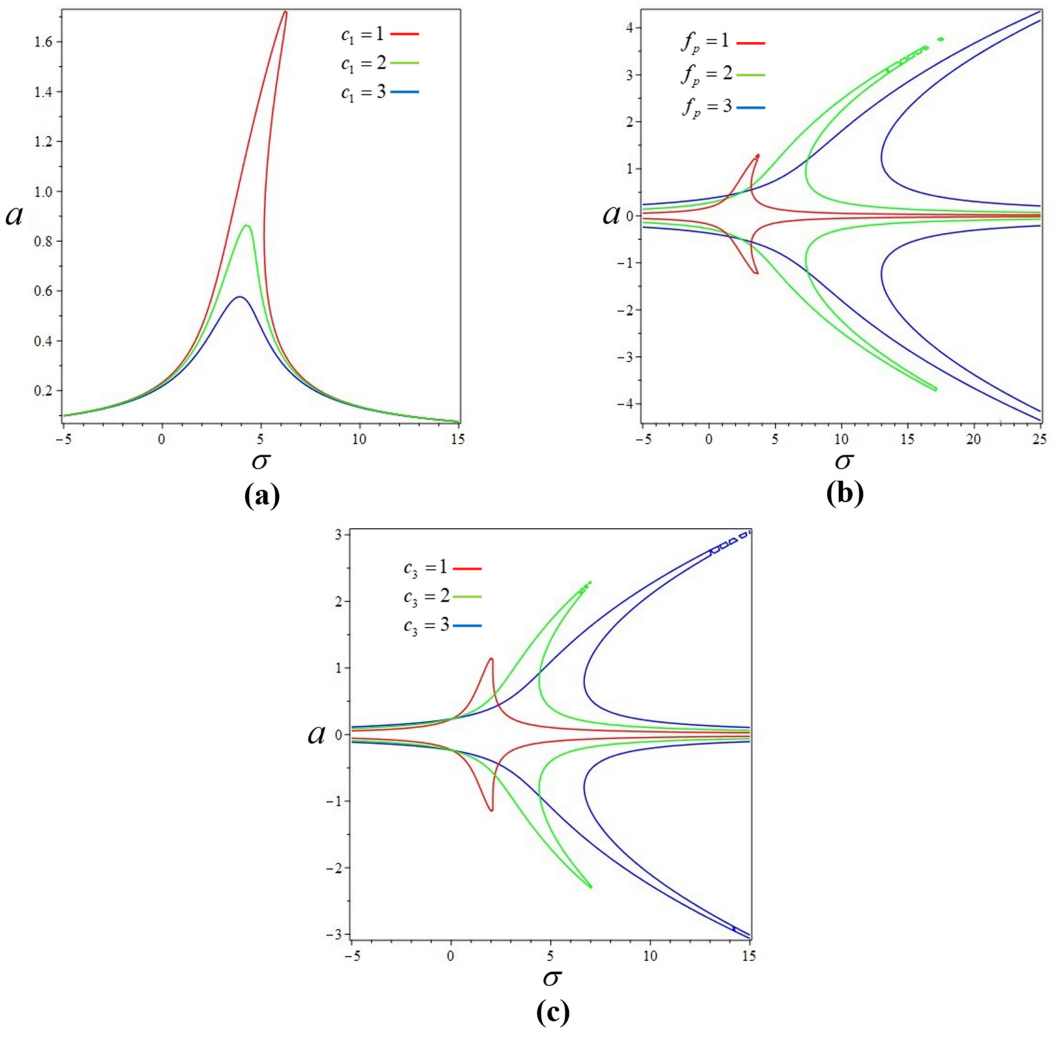
Figure 5 shows the effect of different factors on frequency response during primary resonance. In Figure 5a, when , the amplitude-frequency response curves of the primary resonance of the system under different damping values are shown. It is obvious that with the increase in damping value, the primary resonance amplitude of the system decreases, and the unstable region is gradually narrowing. However, the backbone curve does not change with the damping value. In Figure 5b, when , the amplitude-frequency response curves of the primary resonance of the system under different external excitations are shown. It is obvious that with the increase in the external excitation value, the resonant region of the primary resonance of the system is increasing, and the maximal amplitude is also increasing. The resonant point constantly shifts to the right, increasing the unstable region, but the backbone curve does not change with the damping value. In Figure 5c, when , the amplitude-frequency response curves of the primary resonance of the system under different cubic nonlinear stiffness are shown. With the cubic nonlinear stiffness increase, the resonance point shifts to the right, and the unstable region increases. However, the maximal amplitude of the primary resonance of the system does not change, and the backbone curve tilts right.
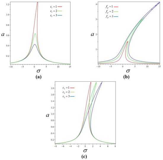
Figure 5.
Frequency response for primary resonance: (a) different damping values, (b) different external excitations, (c) different cubic nonlinear stiffness.
The influence law of primary resonance of drillpipe systems can be obtained by analyzing the above three cases: damping term and external excitation affect the maximum amplitude of primary resonance of the drillpipe system; damping term, external excitation, and cubic nonlinear stiffness coefficient affect the size of instability region of the system; in the unstable region, the system will incur irregular vibrations and even chaos.
When , by using Equation (37), we can obtain
By selecting the parameters in Table 1, the approximate solution of the first-order dynamic response of the primary resonance of the system can be obtained. Figure 6 shows the dynamic response diagram of primary resonance.

Table 1.
Primary resonance dynamic response parameter table.
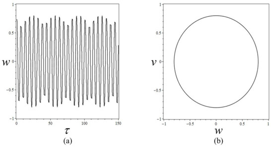
Figure 6.
Dynamic response diagram of primary resonance: (a) diagram of transverse displacement versus time, (b) Phase portrait.
4.2. Secondary Resonances Response
4.2.1. Subharmonic Resonance Response
To investigate the influence of different factors on the subharmonic resonance response of the drillpipe, when we selected different parameters for analysis. Expanding Equation (49) to
For Equation (54), the quadratic term of frequency must have real roots so it can be obtained that
Figure 7a shows the range of values for and that satisfies Equations (55) and (56). Not all tuning parameters and external excitations obviously have subharmonic resonance. With the increase in tuning parameters , under the external excitation within a certain range, the subharmonic resonance of the system will significantly affect the entire drillpipe system. Figure 7b shows the effect of damping on the resonance region. As the damping increases, the curve moves right, and the resonance region becomes smaller. This shows that with the increase in damping value, it requires more significant external excitation and excitation frequency to resonate.
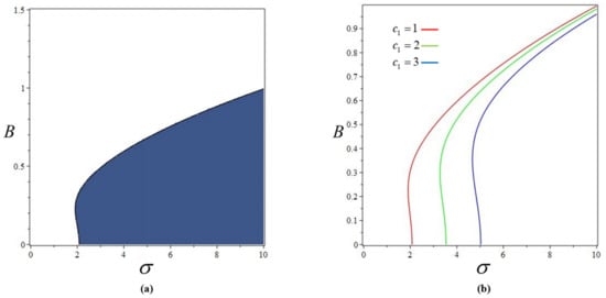
Figure 7.
Range of subharmonic resonance: (a) subharmonic resonance response range, (b) the influence of different damping values on the response range of subharmonic resonance.
Figure 8 shows the effect of different factors on frequency response during subharmonic resonance. In Figure 8a, when , the amplitude-frequency response curves of the subharmonic resonance of the system under different damping values are shown. It is obvious that with the increase in damping, the maximal amplitude of resonance decreases, and the resonance region decreases. In Figure 8b, when , the amplitude-frequency response curves of the subharmonic resonance of the system under different external excitations are shown. Obviously, with the increase in external excitation, the maximal amplitude and resonance region of resonance will decrease. In Figure 8c, when , the amplitude-frequency response curves of the subharmonic resonance of the system under different cubic nonlinear stiffness are shown. It is obvious that with the increase in cubic nonlinear stiffness, the maximum amplitude and resonance region of resonance become smaller.
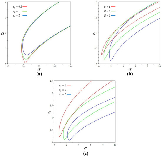
Figure 8.
Frequency response for subharmonic resonance: (a) different damping values, (b) different external excitations, (c) different cubic nonlinear stiffness.
The influence law of subharmonic resonance of the drillpipe system can be obtained by analyzing the above three cases: when the external excitation increases to a certain range, there will be obvious subharmonic resonance with the increase in frequency, and the damping value will shift the range to the right. The damping term, the external excitation, and the stiffness coefficient of the third nonlinear term affect the amplitude and the size of the resonance region of the third harmonic resonance of the drillpipe system.
When , by using Equation (49), we can obtain
By selecting the parameters in Table 2, the approximate solution of the first-order dynamic response of the subharmonic resonance of the system can be obtained. Figure 9 shows the dynamic response diagram of subharmonic resonance.
Table 2.
Subharmonic resonance dynamic response parameter table.
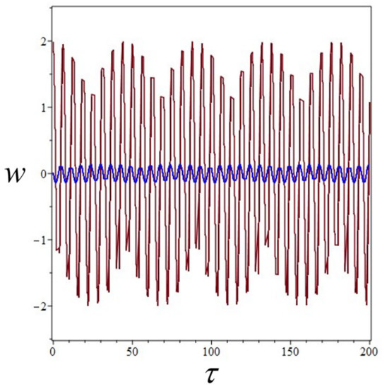
Figure 9.
Dynamic response diagram of third harmonic resonance displacement.
4.2.2. Superharmonic Resonance Response
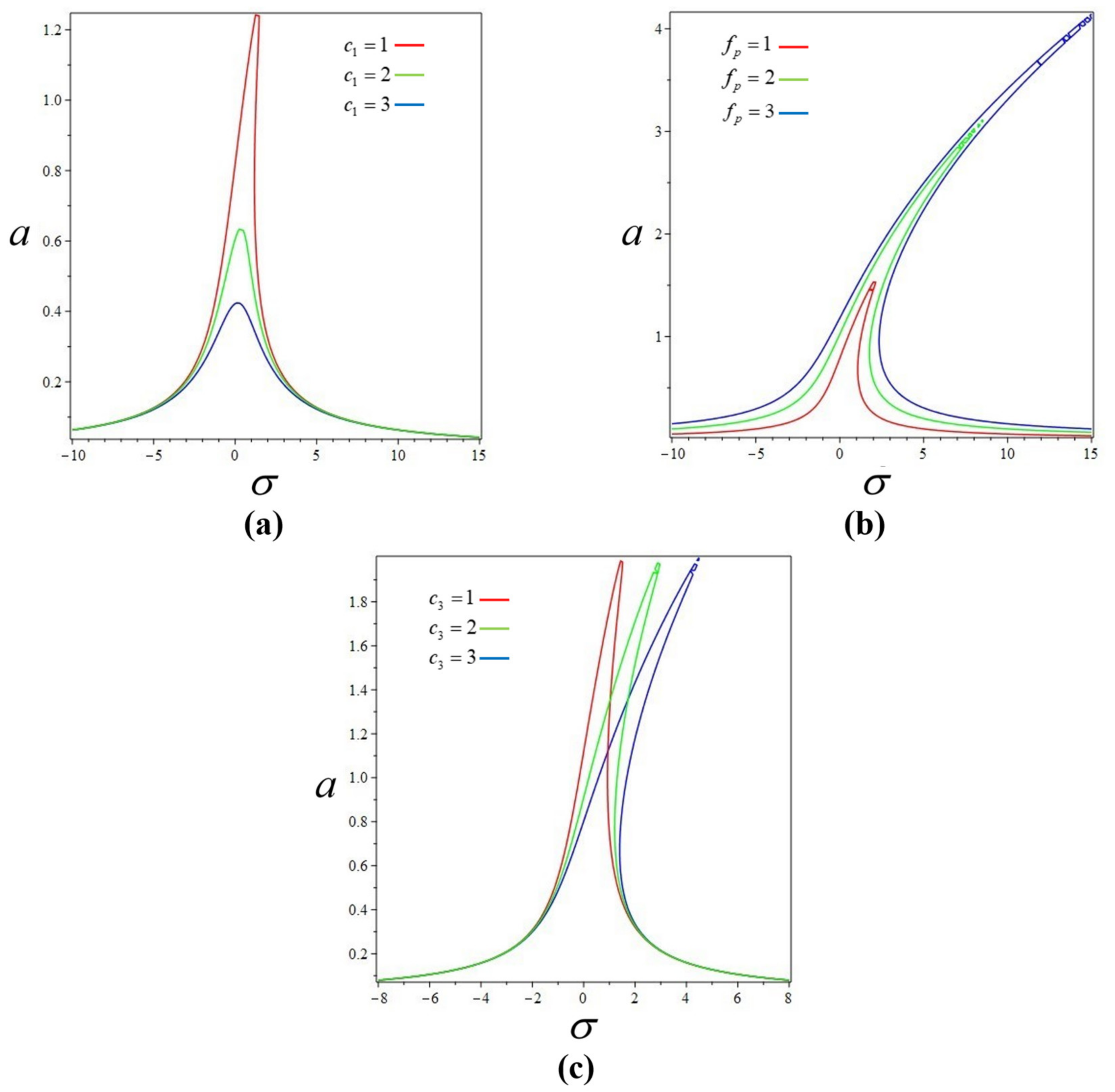
To investigate the influence of different factors on the superharmonic resonance response of drillpipe, when we selected different parameters for analysis.
Figure 10 shows the effect of different factors on frequency response during superharmonic resonance. In Figure 10a, when , the amplitude-frequency response curves of the superharmonic resonance of the system under different damping values are shown. It is obvious that the effect of damping on superharmonic resonance is similar to that of damping on primary resonance. With the increase in damping value, the superharmonic resonance amplitude of the system decreases, and the unstable region is gradually narrowing. However, the backbone curve does not change with the damping value. In Figure 10b, when , the amplitude-frequency response curves of the superharmonic resonance of the system under different external excitations are shown. It is obvious that with the increase in external excitation, the resonance region increases, the maximal amplitude increases, the resonance point shifts to the right, the unstable region increases, and the ridge line of the response curve shifts to the right. In Figure 10c, when , the amplitude-frequency response curves of the superharmonic resonance of the system under different cubic nonlinear stiffness are shown. It is obvious that with the increase in cubic nonlinear stiffness, the resonance point shifts to the right, the unstable region increases, and the maximal amplitude increases.
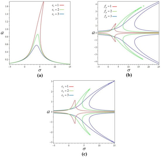
Figure 10.
Frequency response for superharmonic resonance: (a) different damping values, (b) different external excitations, (c) different cubic nonlinear stiffness.
The influence law of superharmonic resonance of drillpipe systems can be obtained by analyzing the above three cases: the damping term, external excitation, and the stiffness coefficient of the third-order nonlinear term jointly affect the amplitude and instability region of the third-order superharmonic resonance of the drillpipe system.
When , by using Equation (52), we can obtain
By selecting the parameters in Table 3, the approximate solution of the first-order dynamic response of the superharmonic resonance of the system can be obtained. Figure 11 shows the dynamic response diagram of superharmonic resonance.
Table 3.
Superharmonic resonance dynamic response parameter table.
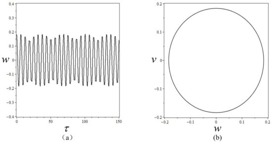
Figure 11.
Dynamic response diagram of superharmonic resonance: (a) diagram of transverse displacement versus time, (b) phase portrait.
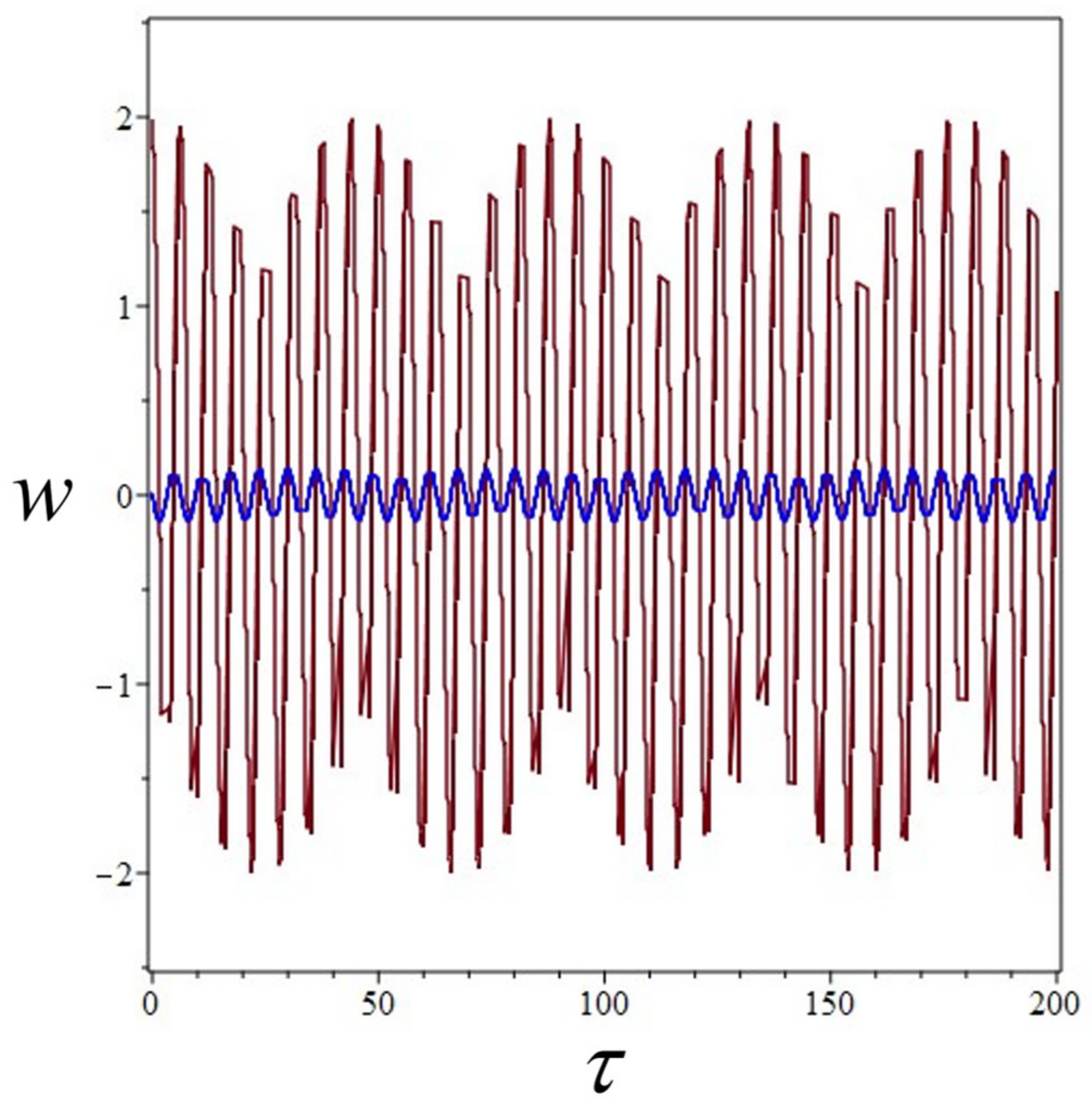
Through the comparison and analysis of the response diagram, the corresponding dynamic laws of the system can be obtained. It can be seen from Figure 6, Figure 9, and Figure 11 that the approximate solution of the nonlinear vibration of the drillpipe is obtained by using the first-order accuracy of the multi-scale method. The displacement dynamic response curves of the three resonances have similar variation laws of chord function, but the amplitude and phase angle of the three resonance response curves differ. In general, the dynamic response law of the primary resonance is similar to that of the third-order superharmonic resonance.
The comparison between Figure 6a and Figure 11a shows that under the same parameters, the dynamic response of the primary resonance displacement is significantly greater than that of the third-order superharmonic resonance. This indicates that the effect of the primary resonance is the most obvious in the three resonances when resonance occurs. The difference in the phase angle makes the maximum displacement caused by the primary and third-order superharmonic resonance appear alternately in the resonance problem. Figure 6 and Figure 11 show that the resonance phenomena of the primary resonance and the third-order superharmonic resonance under the selected parameters are stable periodic motions.
Figure 9 shows that when the third subharmonic resonance occurs in the system with the increase in external excitation, the dynamic response of displacement has two solutions, and the dynamic response of displacement may jump between the two amplitudes, indicating that the system will be in an unstable state when the third subharmonic resonance occurs.
5. Summary
In this paper, the authors considered the damping and external excitation of mud, introduced the nonlinear term of the third contact force between coring drillpipe and core, and established a reduced-order model of coring drillpipe. The study of the system′s primary and harmonic resonance shows that the damping term has a significant inhibitory effect on the amplitude of resonance, and external excitation affects the intensity of resonance when the drilling speed and pressure are constant. Research also shows that the resonance of the drillpipe is intensified due to the core limitation.
From the analysis of the three resonance problems, it can be known that under specific system parameters, the subharmonic resonance of the drill pipe system is more unstable. Still, the primary resonance is the strongest, indicating that the vibration caused by the primary resonance will be more intense. It suggests that the drilling parameters should be changed to keep the system from the influence of the primary resonance. These findings are helpful for field drilling, and changing the corresponding parameters can avoid the adverse effects of resonance. Appropriately increasing the viscosity of mud and reducing the value of external excitation are effective means to reduce the resonance amplitude. These findings also help design coring tool combinations. For example, increasing the distance between the core and the core tube can avoid more intense resonance of the core tube. Appropriately increasing the stiffness of the drill pipe can make the drill pipe away from the resonance region. These proposals can effectively improve drilling efficiency, reduce downhole accidents, reduce labor intensity, and reduce drilling cost.
Author Contributions
Conceptualization, Y.S., Y.L. and G.Y.; Data curation, X.Q.; Formal analysis, Z.F.; Funding acquisition, Y.L.; Methodology, Y.L.; Software, Y.S.; Visualization, Z.D.; Writing—original draft, Y.S.; Writing—review & editing, Y.L., X.Q., Z.D. and Z.F. All authors have read and agreed to the published version of the manuscript.
Funding
The research was funded by the Natural Science Foundation of China (No. 42002307), Fundamental Research Funds for the Central Universities, China (No. 2652019070).
Institutional Review Board Statement
Not applicable.
Informed Consent Statement
Not applicable.
Data Availability Statement
Not applicable.
Acknowledgments
The authors gratefully acknowledge the financial support from the Natural Science Foundation of China (No. 42002307), Fundamental Research Funds for the Central Universities, China (No. 2652019070).
Conflicts of Interest
The authors declare no conflict of interest.
References
- Ahmed, U.; Meehan, D.N. Unconventional Oil and Gas Resources: Exploitation and Development; CRC Press: Boca Raton, FL, USA, 2016. [Google Scholar]
- Teodoriu, C.; Bello, O. An Outlook of Drilling Technologies and Innovations: Present Status and Future Trends. Energies 2021, 14, 4499. [Google Scholar] [CrossRef]
- Nikolaos, P.P. An Approach for Efficient Analysis of Drill-String Random Vibrations; Dissertation, Taxes; Rice University: Houston, TX, USA, 2002. [Google Scholar]
- Ritto, T.G.; Soize, C.; Sampaio, R. Non-linear dynamics of a drill-string with uncertain model of the bit-rock interaction. Int. J. Non-Linear Mech. 2009, 44, 865–876. [Google Scholar] [CrossRef] [Green Version]
- Apostal, M.C.; Haduch, G.A.; Williams, J.B. A Study to Determine the Effect of Damping on Finite-Element-Based, Forced-Frequency-Response Models for Bottomhole Assembly Vibration Analysis. In Proceedings of the SPE Annual Technical Conference and Exhibition, New Orleans, LA, USA, 23–26 September 1990. [Google Scholar]
- Jansen, J.D. Non-Linear Rotor Dynamics as Applied to Oilwell Drillstring Vibrations. J. Sound Vib. 1991, 147, 115–135. [Google Scholar] [CrossRef]
- Vaz, M.A.; Patel, M.H. Analysis of Drill Strings in Vertical and Deviated Holes Using the Galerkin Technique. Eng. Struct. 1995, 17, 437–442. [Google Scholar] [CrossRef]
- Khulief, Y.A.; Al-Naser, H. Finite Element Dynamic Analysis of Drillstrings. Finite Elem. Anal. Des. 2005, 41, 1270–1288. [Google Scholar] [CrossRef]
- Omojuwa, E.O.; Osisanya, S.; Ahmed, R. Influence of Dynamic Drilling Parameters on Axial Load and Torque Transfer in Extended-Reach Horizontal Wells. In Proceedings of the SPE Annual Technical Conference and Exhibition, ATCE 2014, Amsterdam, The Netherlands, 27–29 October 2014. [Google Scholar]
- Zhao, Z.B.; Qiu, X.Q.; Xu, J.L. Finite element analysis of modal vibrations of drill strings in deep-sea natural gas hydrate coring/drilling. Nat. Gas Ind. 2011, 1, 73–76. [Google Scholar]
- Liang, J.; Guo, B.K.; Wang, Z.G.; Sun, J.H.; Li, X.M.; Yin, H. Dynamics Behavior of Compound Drill String for Wire-line Coring. Explor. Eng. 2017, 44, 34–40. [Google Scholar]
- Liu, Y.S.; Gao, D.L.; Vipin, A. Drillstring Oscillations: The Influence of Fluid Loading and Stabilizer Effects. Shock Vib. 2021, 2021, 8888837. [Google Scholar] [CrossRef]
- Kamgue, L.; Arnaud, R.; Deng, J.; Feng, Y.C.; Li, H.T.; Oloruntoba, A.; Songwe, S.; Naomie, B.; Marembo, M.; Sun, Y.X.; et al. Numerical Investigation of the Influence of the Drill String Vibration Cyclic Loads on the Development of the Wellbore Natural Fracture. Energies 2021, 14, 2015. [Google Scholar] [CrossRef]
- Païdoussis, M.P.; Li, G.X. Cross-flow-induced chaotic vibrations of heat-exchanger tubes impacting on loose supports. J. Sound Vib. 1992, 152, 305–326. [Google Scholar] [CrossRef] [Green Version]


Publisher’s Note: MDPI stays neutral with regard to jurisdictional claims in published maps and institutional affiliations. |
© 2022 by the authors. Licensee MDPI, Basel, Switzerland. This article is an open access article distributed under the terms and conditions of the Creative Commons Attribution (CC BY) license (https://creativecommons.org/licenses/by/4.0/).