Article

A Computational Method of Rotating Stall and Surge Transients in Axial Compressor

Jiangsu Province Key Laboratory of Aerospace Power System, College of Energy and Power Engineering, Nanjing University of Aeronautics and Astronautics, Nanjing 210016, China
*
Author to whom correspondence should be addressed.
Energies 2022, 15(14), 5246; https://doi.org/10.3390/en15145246
Submission received: 27 June 2022 / Revised: 8 July 2022 / Accepted: 12 July 2022 / Published: 20 July 2022

Abstract

:
The onset of rotating stall and surge in compressors limits the operating range of aero-engines. Accurately predicting the key features during these events is critical in the engine design process. In this paper, a three-dimensional computational model for transient simulation of multi-stage axial compressors during stall is proposed. The kinetic equations describing the dynamic process of the compression system are constructed, with a 3D through-flow model for the compression part and a 1D gas collector model for the outlet part. The calculation of the source term is performed using the developed body-force model, which realizes the correlation between the deviation angle and the loss coefficient with the inlet parameters in various flow regions. Validated on a single-stage compressor and a single-rotor fan, the results show that the method is capable of capturing the stall and surge features correctly and that the three-dimensional structure of the stall cell can be captured. In addition, this model could be used for the analysis of the surge load, which is significant for the structural integrity of the compressor.

1. Introduction

The compressor is a key component of an aero-engine, and its aerodynamic instability problem has an important impact on the performance and reliability of the whole engine. As the flow through the compressor decreases, the compressor works away from its design point, even as its internal steady flow is disrupted. After crossing the stability boundary, the compressor will enter an unstable state, such as rotating stall and surge. In many cases, the consequences associated with the onset of stall are quite severe. The flow rate and pressure rise decrease significantly and the efficiency drops dramatically. There can be a significant lag between the start and the stop of stall, which can seriously affect the recovery of the compression system from stall. In addition, stall will cause forced vibration of the compressor rotor blade, which increases the vibration stress of the blade and damages its structural integrity. As a result, designers often sacrifice compressor performance during the design process to maintain stall margins. Therefore, the study and control of the stall phenomenon have always been an important part of the design of aero-engine compressors. Numerous solutions have been investigated to suppress the occurrence of compressor stall and to increase surge margin. Such as axisymmetric arc-shaped slots casing treatment investigated by Pan et al. [1], the ported shroud was developed by Cravero et al. [2] and radial injectors were tested by Khaleghi [3].
Rotating stall is usually described as consisting of several stall cells covering part of the blades, and the stall cells rotate in the direction of rotor rotation at part of the rotor rotational speed. Surge is an unstable flow state characterized by interruption of airflow in the entire compression system consisting of the compressor, its inlet and outlet piping, downstream throttling devices, etc. [4]. Rotating stall is always accompanied by a sudden drop in pressure rise, and stall occurs close to the peak of the total-static pressure rise characteristic [5]. Once stall is fully developed, the circumferential averaged mass flow and pressure ratio remain almost constant. These features provide the basis for judging, as well as simulating the occurrence of stall. Greitzer [6,7] proposed the well-known B-parameter, which correlates rotating stall with surge. Greitzer’s experiments have shown that the compression system has a critical B-parameter, above which surge will occur and below which rotating stall will occur. Rotating stall is a disturbance of the flow in the tangential direction, while surge is a disturbance in the axial direction, and which form of disturbance dominates is influenced by the length and volume of the overall compression system [5]. Greitzer’s work established the basis for a unified simulation of rotating stall and surge, and many simulations since then have borrowed this idea.
There is a certain risk involved in the experimental study of the post-stall phenomenon. When the compression system enters an unstable operating condition, it can be very destructive to the system, especially the phenomenon of surge, more so when experiments are conducted on a multi-stage axial compressor with a high speed and high-pressure ratio. Therefore, reliable numerical calculations are required to be utilized. Ideally, designers would like to be able to perform time-accurate, high-resolution calculations for the whole compression system for the complete duration of stall or surge. The three issues that make this a challenging aerodynamic problem are the estimation of the steady-state performance, the prediction of the stability boundary, and the calculation of the subsequent growth of the flow field perturbation into either mature rotating stall or a surge cycle [8]. One of the most common methods for obtaining high-resolution calculations of multi-stage axial compressor performance is three-dimensional computational fluid dynamics (CFD). Recently, extensive work on this part has been done by Moreno [9] and Zhao [10] and others, especially for multi-stage high-pressure compressors. Huang [11] et al. established a 1D–3D coupled method for simulating compressor surge in a compression system. However, simulating rotating stall and surge using Navier–Stokes (URANS) requires full-annulus grids as well as small time steps, which are often time-consuming for typical multi-stage pressurizers.
Therefore, the designers developed a series of simplified models to simulate the aerodynamic processes during the stall and surge transients. Greitzer [6,7] presented the definitive work on surge and established a lumped parametric model. Moore and Greitzer [12,13] gave a unified view of stall and surge in multistage compressors, coupling a two-dimensional representation of the unsteady flow in the compressor with the lumped parametric model of the entire system to achieve a dynamic process simulation of the compression system. Bonnaure [14] developed a 2D model similar to Moore and Greitzer and considered the effect of compressibility. However, these models cannot describe the flow field between the blade rows. Takata and Nagano [15] developed a two-dimensional incompressible unsteady model that simulates the row with an excitation disk, and this model could be used to predict the onset of stall, the development of the stall cell, and the rate of propagation. However, such models still cannot simulate the flow within the blade row. The current trend regarding the simulation methods for post-stall dynamic processes is to use a body-force model, where the action of the blade profile on the airflow is modeled as the body force source term in a three-dimensional equation that allows describing the flow in the blade channel. Escuret and Garnier [16] were the first to simulate aerodynamic instability using Euler’s equation with source terms derived from correlations and considered a large one-dimensional plenum chamber downstream, which allows simultaneous simulation of rotating stall and surge. Gong [17] described a three-dimensional unsteady computational model based on the channel-averaged body force, using a form similar to the drag coefficient and the pressure rise coefficient to calculate the force parallel to and perpendicular to the flow direction, which can describe the spike-like stall inception, part-span rotating stall, etc. Chima [18] developed a three-dimensional model, CSTALL, which calculates the body force from the amount of change in velocity annulus and entropy increase at the inlet and outlet of the blade row. The model can preliminarily predict and analyze the onset of stall. Longley [8] proposed a new method for predicting the occurrence of highly separated flow during stall by adding an equation that allows obtaining the airflow parameters during highly separated flow. Righi et al. [19,20] established the three-dimensional model ACRoSS, where the calculation of the source term extended the assumptions of Longley [8] et al. and can be used to calculate rotating stall and surge of the multistage compressor. Zeng [21] et al. developed a new body-force model to capture the three-dimensional and unsteady features of stall and surge in compressors with Thomason and Moses’s model [22].
Obviously, the key to such models is the simulation of blade forces, especially the flow field parameters associated with them, such as loss coefficient and deviation angle. These parameters are provided by correlations, which are often adapted for different flow conditions. There are few studies related to the loss coefficient and deviation angle during stall and reverse flow. Thomason and Moses [22] obtained the deviation angle and loss coefficient of the separation flow under the large attack angle by some assumptions. Tauveron [23] proposed a new correlation to estimate the steady-state characteristics of the compressor in the whole flow region. Longley [8] introduced a variable which captures the non-uniformity of the flow and can adequately capture the loss and deviation angle during reverse flow. However, the variation form of deviation angle and loss coefficient under large separation is still not known, and the models used for various flow cases are not continuous. Discontinuous processing makes it impossible to use a unified model for steady-state characteristics and post-stall calculations, which may lead to inaccurate predictions for stable boundary points and even to non-physical effects.
In this paper, the three-dimensional compressor computational domain is coupled with the one-dimensional gas collector model, and the through-flow computational method is combined with the developed body-force model to establish a three-dimensional computational model that can be used to simulate the dynamic process of post-stall in the multi-stage compressor. The model is based on the local flow variables, correlating the source term with the local flow field parameters in a way that the correlation is continuous in different flow regions. It is a model integrating characteristic calculation and post-stall calculation. The blade aerodynamic load in the process of surge can be easily obtained. Besides, it takes less time compared to the RANS method. The second part will specify this modeling approach, and the third part will verify the simulation capability of this model with two computational examples.

2. Methodology

A three-dimensional through-flow code has been developed to model compressor rotating stall and surge. The internal flow field of a compressor is described by solving a three-dimensional set of unsteady equations with source terms in the absolute cylindrical coordinate system. In the blade region, the effect of the blade profile on the airflow is replaced by the body force source term, which is the main idea of the body-force model. Assuming that the flow is locally axisymmetric, the blade blockage factor b is used to reflect the effect of the finite thickness of the blade on the flow in the blade region. This treatment avoids the complex meshing effort resulting from direct consideration of the blade profile, and thus allows the large-scale features of the flow within the turbomachinery to be quickly captured with relatively regular coarse meshes. This section first introduces the governing equations and then describes the blade-force modeling method as well as the correlation method.

2.1. Governing Equations

The governing equations to be solved in the bladeless zone and the bladed zone are shown in Equations (1) and (2), respectively. In order to consider the energy exchange between different streamlines in the main flow region due to turbulent diffusion, the turbulent viscous stress τ and turbulent heat transfer term q are introduced in the set of Euler equations to describe the phenomenon based on the dominant idea of Gallimore’s [24,25] spanwise mixing model.
U t + E E v z + 1 r F F v θ + 1 r r G G v r = S
b U t + Ω b U θ + b E E v z + 1 r r b G G v r = b S + S b + b S F
U = ρ ρ v z ρ v θ ρ v r ρ e E = ρ v z ρ v z 2 + p ρ v θ v z ρ v r v z v z ρ e + p F = ρ v θ ρ v z v θ ρ v θ 2 + p ρ v r v θ v θ ρ e + p G = ρ v r ρ v z v r ρ v θ v r ρ v r 2 + p v r ρ e + p E v = 0 τ z z τ z θ τ z r i = 1 3 τ z i v i q z F v = 0 τ θ z τ θ θ τ θ r i = 1 3 τ θ i v i q θ G v = 0 τ r z τ r θ τ r r i = 1 3 τ r i v i q r S = 0 0 ρ v θ v r + τ r θ r ρ v θ 2 + p τ θ θ r 0 S b = 0 p b z 0 p b r 0 S F = 0 F z F θ F r F θ Ω r
where U is the vector of conserved variables, E, F, and G are the inviscid convective flux, E v , F v , and G v are the viscous diffusion flux, S is the centrifugal force and Coriolis force source term derived from the flow equation in the cylindrical coordinate system, S b is the blockage term which represents the influence of the finite thickness of the blade profile, and S F is the source term that characterizes the effect of the blade profile on the flow.

2.2. Blade Force Model

For the calculation in Equation (2), based on Marble’s idea [26], this model decomposes the body force into two parts: one for the non-viscous force perpendicular to the relative velocity and the other for the viscous force inverse and parallel to the relative velocity, as shown in Equations (3)–(5).
F = φ + f = φ z φ θ φ r + f z f θ f r
f // w f z f θ f r = f w v z v θ Ω r v r
φ w φ z v z + φ θ v θ Ω r + φ r v r = 0
The vicious blade force is mainly used to model the airflow losses associated with the flow caused by the blade boundary layer, and the main principle for modeling this part of the force is to ensure that all the work it does is used to generate the entropy of the airflow. Then the magnitude of the viscous force is:
f = ρ T v m w s m
The inviscid blade force is mainly used to reflect the turning effect of the blade on the airflow, i.e., the flow direction of the airflow in the blade area will be controlled by the inviscid blade force. Firstly, under the assumption of steady-state and local axisymmetry, the total circumferential force of the blade is obtained from the circumferential momentum equation with the introduction of the target circumferential velocity.
F θ = φ θ + f θ = 1 b b ρ v z v θ target τ z θ z + 1 b r r b ρ v θ target v r τ r θ r ρ v θ target v r r + τ r θ r
where v θ target is obtained by the instantaneous meridional velocity, the local metal angle, and the deviation angle. In addition, it relates the inviscid radial force and circumferential force to the shape of the mid-camber of the blade profile.

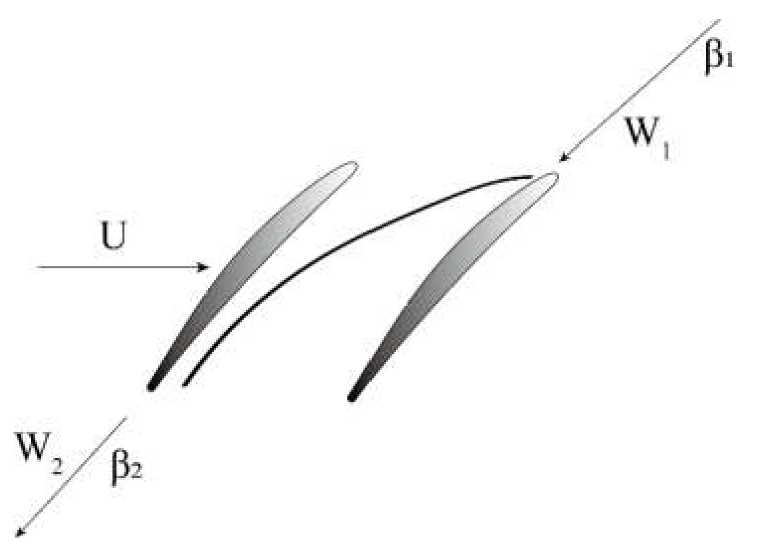
2.3. Elementary Cascade Characteristics

Based on the above analysis, as long as the loss coefficient and the deviation angle of the blade row are determined, combined with the local instantaneous flow parameters, S F can be determined by combining relevant equations. Therefore, the relationship between the body force source term and the upstream flow parameters can be established indirectly as long as ϖ and δ are associated with the inlet flow parameters of the blade elementary channel. Here, the distinction regarding different flow patterns is judged by attack angle. For flow with small attack angles, the relationship between the deviation angle and loss coefficient of the elementary channel with different blade height and its inlet attack angle and Mach number is established through an empirical correlation-based deviation angle and loss model [27], which is not the focus of this paper and therefore not discussed. For flow with large attack angles, the idea of the elementary cascade method is still used because it represents the basic characteristics of the blade flow, which itself is axisymmetric. This treatment makes the calculation method for different flow regions continuous, which will be more accurate for the determination of steady-state boundary.
With reference to the small attack angle region, there is still given a set of relations between the deviation angle and the loss coefficient with the flow parameters at the inlet of the blade elementary flow channel. The range of parameter constraints is first calculated, and the flow in the elementary flow channel is shown in Figure 1, which must satisfy β 2 β 1 by the expansive nature of the compressor channel. For loss coefficient, it is generally accepted that 0 ϖ 1 . When stall occurs, it is always accompanied by a large separation of the flow field and a sudden increase in deviation angle and loss; when the channel is completely blocked, the deviation angle and loss are considered to be no longer changing. Based on this assumption and some results from the RANS calculation of the two-dimensional blade cascade, the distribution of the deviation angle and the loss coefficient can be given within the constraint. The given deviation angle and loss characteristics both increase first and then remain constant, with a larger increase compared to the small attack angle region. A schematic diagram of the curve shape is shown in Figure 2. The parameter values are different for different blade height positions.

2.4. Unsteady Treatment

When rotating stall or surge occurs in the compressor, the flow is unsteady. The difference between unsteady flow and quasi-steady flow is the dynamic hysteresis effect. Referring to the treatment of Longley [8], the bound circulation approach is used here, and the steady-state bound circulation is defined as follows.
Γ s s = φ θ s s / ρ v m
In unsteady flow any change in the bound circulation results in shed circulation, which is then convected through the blade passage by the local flow. Until the shed circulation is far downstream, it affects the local blade force. The first-order time-lag mode is introduced and the information transfer with the rotation of the blade row is considered:
τ φ θ t + Ω φ θ θ = φ θ s s φ θ
where the time constant τ is calculated from the blade meridional length and the instantaneous meridional velocity. For the stator blade row, the rotational speed Ω is equal to 0.

2.5. Initial Boundary Conditions

The initial condition of this model is the steady-state operating point of the compression system. Four types of boundaries are modeled here: wall, rotationally periodic, inflow, and outflow. The wall boundary conditions are assumed to be slip-wall. The inlet boundary conditions specify the total temperature, total pressure, and flow angle. The outlet boundary condition is obtained from the valve function. The valve is modeled with the classical throttle model, where the pressure drop is proportional to the quadratic side of the mass flow rate. Then the outlet pressure can be calculated as
p e = p 0 + k m ˙ t 2
where p 0 is atmospheric pressure, k is the throttle coefficient and m ˙ t is compressor outlet mass flow rate.

2.6. Numerical Solution Method

Equations (1) and (2) are discretized using the cell-centered finite volume method. A four-stage explicit Runge–Kutta scheme [28] is used to solve the time terms. Spatial items are treated with a low-diffusion flux-splitting scheme (LDFSS) [29]. For the calculation of steady-state characteristics, only one grid is used in the circumferential direction because the flow is axisymmetric. When approaching the stall boundary, multiple grids are used in the circumferential direction. In order to develop a physically correct rotating stall cell in the compressor, some asymmetry must be introduced artificially. The methods to introduce asymmetry include introducing random disturbance in the flow field or slightly changing the geometry of the compressor. In the current simulation, within 0.1 rotor rotating cycle, a small sinusoidal disturbance is applied to the total pressure at the inlet of the calculation domain, with an amplitude of 0.05% of atmospheric pressure and a wavelength of the rotor circumference, which is sufficient to produce rotating stall.

3. Model Validation

3.1. Single-Stage Compressor

The geometric parameters of the single-stage compressor are shown in Table 1, and the meridional flow path is shown in Figure 3. The rotational speed of the compressor in the experiment and calculation is 1000 r/min.

3.1.1. Steady-State Calculation

Since the flow is axisymmetric, the steady-state characteristics are calculated using only one grid in the circumferential direction. The valve coefficient is gradually increased to approach the stability boundary. Figure 4 shows the calculated total-static pressure rise characteristics obtained with the experimental results, both of which are very close. The flow coefficient and the total-static pressure rise coefficient are defined as follows.
φ = v z U ,   ψ t s = p o u t l e t p 0 i n l e t 1 2 ρ U 2

3.1.2. Rotating Stall Simulation

A small sinusoidal disturbance is applied to the compressor inlet and the valve coefficient is increased. When the valve coefficient is 0.0167, the flow rate and the total-static pressure rise coefficient change abruptly, and the flow coefficient before the rotor versus time is shown in Figure 5. The final flow coefficient remains unchanged, and this final state is referred to as the “stable characteristic point”. As shown in Figure 6, comparing the stable characteristic point with the experimental results, it is found that they are very close. Table 2 shows the values of the parameters obtained experimentally and calculated for the two operating points, as well as the percentage errors.
The calculated traces of static pressure in the tip region of the compressor inlet at different circumferential locations are shown in Figure 7a, which can be determined that a rotating stall has occurred, and the rotational speed of the stall cell is 33.21% of the rotor rotational speed. The experimental results are shown in Figure 7b, and it can be seen that the calculated and experimental results are very close in terms of the static pressure variation during stall as well as the rotational speed of the stall cell.
Figure 8 shows the axial velocity at the inlet and outlet of each blade row when the stall cell is fully developed, and Figure 9 shows the axial velocity contour on unwrapped surface at midspan of the compressor. It can be seen that the distribution of the stall cell is wide, and the stall cell occupies about 50% of the circumference.
Figure 10 shows the variation of the axial velocity in the inlet and outlet of the rotor and stator row at the tip and hub, from which it can be seen that the axial velocity fluctuates most at the rotor tip as well as the stator hub, i.e., the stall cell has the greatest influence on the two locations. Figure 11 shows the circumferential distribution of axial velocity at the tip of the leading edge of the rotor at several time points, with the waveform gradually shifting from a sinusoidal wave and increasing in amplitude.

3.2. Single Rotor of the Fan

Since surge is an unstable flow state characterized by airflow interruption in the entire compression system consisting of the compressor and its inlet and outlet piping and downstream throttling devices, etc., and Moore and Greitzer’s study unifies rotating stall and surge, both can use a unified compression system. A plenum-throttle boundary condition is implemented combining with the 3D through-flow model, and similar treatments can be found in the literature [16,30], among others. The computational model is shown in Figure 12.
The downstream component is modeled as a plenum plus valve, assuming that the flow in the plenum is compressible, unsteady, and uniformly distributed. The pressure in the plenum can be calculated from the continuity equation as follows.
d p p l d t = m ˙ c m ˙ t γ R T p l / V p l
where p p l and T p l are the pressure and temperature in the plenum, V p l is the volume of the plenum, and m ˙ c and m ˙ t are the mass flow into and out of the plenum, respectively. In the calculation, the pressure in the plenum is set as the static pressure at the middle diameter of the compressor outlet.
The research object is a single-rotor fan whose design speed is 11,870 r/min. The meridional flow channel and grid are shown in Figure 13. There are 20 grid elements along the radial direction for the whole compressor and 30 grid elements along the axial direction in the rotor region.

3.2.1. Steady-State Calculation

First is the result of steady-state calculation, the volume of the plenum is set to 0.01 m3. Similarly, only one grid is used in the circumferential direction, and the valve coefficient is given as a certain value for the calculation, gradually increasing the valve coefficient until stall occurs, and the steady-state characteristics obtained from the calculation are shown in Figure 14. When the valve closes further, the flow field is not uniform circumferentially, that is, the occurrence of rotating stall, while the last calculation point can be determined as a stable boundary point.

3.2.2. Rotating Stall Simulation

Increasing the valve coefficient, the calculation converges after about 14 rotor rotating cycles, as can be seen in the graph of the flow coefficient versus time in Figure 15. The total-static pressure rise coefficient varies with the flow coefficient, as shown in Figure 16. The black line is the steady-state characteristic line and the purple line is the dynamic process which eventually converges to a point. The calculated axial velocity variation with time in the tip region of the compressor inlet at different circumferential locations is shown in Figure 17, and it can be found that the introduced random disturbance quickly develops into rotating stall.

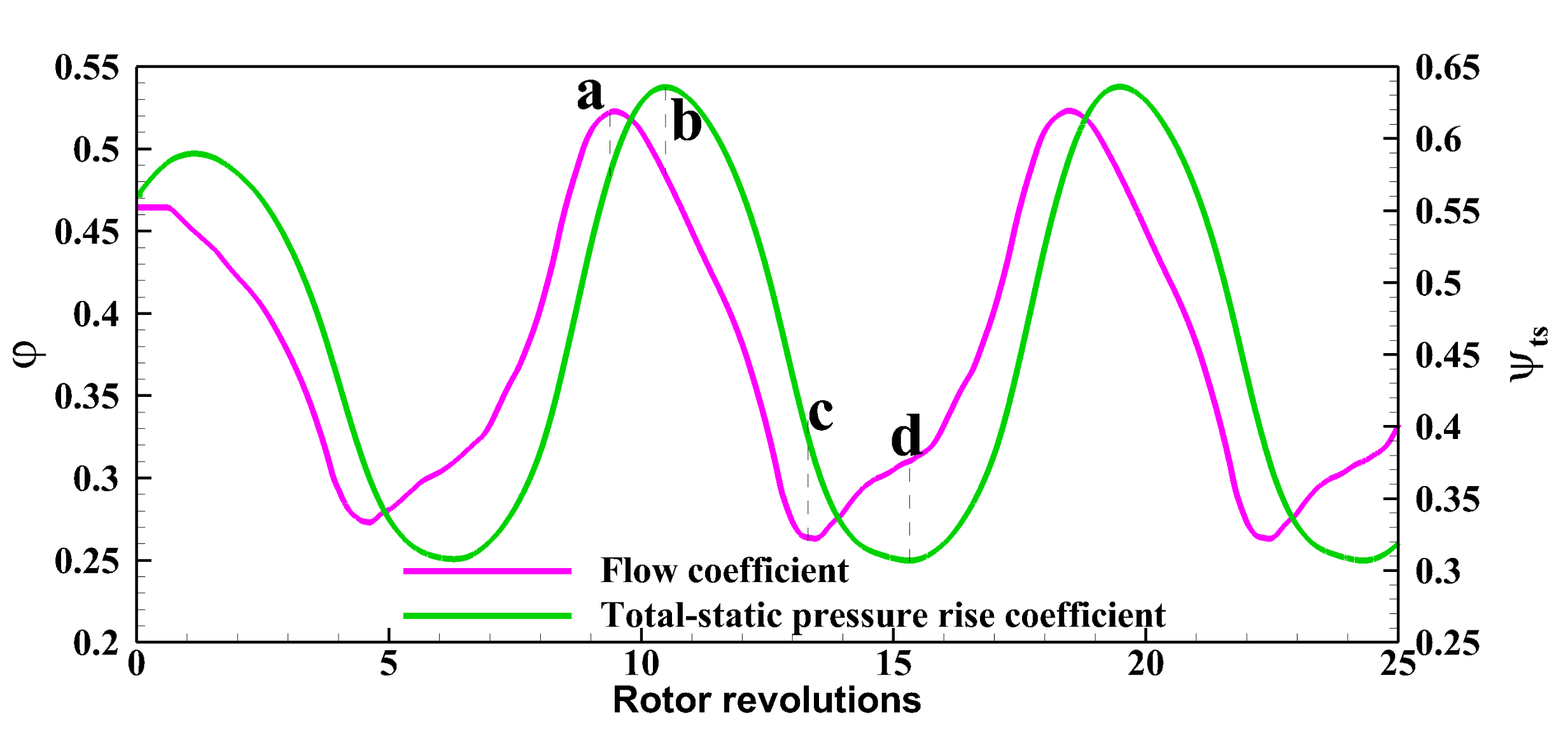
3.2.3. Surge Simulation

The volume of the plenum is increased to 1 m3, and the other settings are kept the same. Unsteady simulation is performed at a certain valve opening, and the flow coefficient and the total-static pressure rise coefficient are plotted against time in Figure 18. As can be seen, the flow coefficient and the total-static pressure rise coefficient oscillate in large magnitudes with a period of about 9 rotor rotating cycles and a frequency of 21.9 Hz. At point a, the flow coefficient reaches the maximum, and the compressor exhausts to the plenum, resulting in the continuous increase of the plenum pressure, which is transmitted to the compressor outlet by the pressure wave so the compressor outlet pressure also increases. At point b, the plenum pressure reaches the peak value. Because the plenum pressure is higher than the pressure rise that the compressor can provide, there is reverse pressure and the flow decreases continuously. When the instantaneous flow reaches the minimum value at point c, the pressure in the plenum decreases gradually because the flow rate through the compressor is much smaller than the flow rate through the throttle. When the pressure in the plenum reaches the minimum value at point d, the pressure rise that the compressor can provide is much greater than the pressure drop of the throttle at the same flow rate, so the flow rate through the compressor increases rapidly; After reaching point a, the above dynamic process is repeated due to instability. Figure 19 shows the variation of total-static pressure rise coefficient with flow coefficient, from which the “surge ring” can be clearly seen. During surge, the circumferential parameters of the compressor are uniform, that is, the rotating stall is not induced.
The prediction of blade load during surge is a challenging task. In the literature, the blade load during surge is often referred to as the “surge load”. It would be important for the structural integrity of the compressor to be able to predict the surge load in the numerical calculation during the design phase. It can be obtained by using the blade force derived from the body-force model. Figure 20 shows the variation of rotor blade force in three directions during surge, where the blade force refers to the force of each rotor blade and is dimensionless to the blade force in three directions at the last stable calculation point, respectively, defined as follows
F ˜ i = F i t F i , n s
It can be seen that the three forces vary periodically and their periods coincide with the surge period, from which the phase variations can also be observed.
Increasing the volume of the plenum, the relationship between the surge frequency and the volume of the plenum was obtained, as shown in Figure 21. As the volume of the plenum increases, the surge frequency decreases, and although some values are slightly higher than 3–10 Hz generally given [31], the variation pattern is consistent with Day’s measurements [32]. Thus, the model can correctly predict the features associated with surge.

4. Conclusions

In this paper, a new body-force model for rotating stall and surge simulation of axial compressors is proposed and validated with two cases. Three-dimensional compressor computational domain is coupled with the one-dimensional gas collector model to simulate rotating stall and surge at the same time. It is a model integrating characteristic calculation and post-stall calculation. Besides, the proposed model can effectively reveal the three-dimensional large-scale flow features of the compressor stall process within a limited time cost. The model is applicable to both low and high-speed compressors. Only single-stage compressors have been validated so far, but it can be extended to multi-stage compressors in the future. The main conclusions are as follows:
  • The relationship between deviation angle and loss coefficient with attack angle for large attack angle flow regions is proposed for simulating typical three-dimensional flow features that occur during rotating stall and surge. Since the deviation angle and the loss coefficient are calculated in the same way as in the case of small attack angles, there will be no physical discontinuity in the transition from unstalled to stalled flow, which will be more accurate for the judgment of the stability boundary.
  • The model is applied to a single-stage axial compressor and compared with the experimental results to verify the accuracy of the steady-state flow field simulation. Further computational analysis shows that the model can simulate rotating stall, and the post-stall stability characteristic and the rotating frequency of the stall cell are predicted with good precision. In addition, due to the three-dimensional nature of the model, it can be used to observe the three-dimensional features of the stall cell.
  • The simulation of rotating stall and surge of a single rotor fan is investigated by coupling the developed three-dimensional body-force model with a one-dimensional gas collector model. The calculations show that the model can still simulate the features related to rotating stall and can simulate the “surge ring” during surge. This model can also be used to calculate the blade load during surge, which will be an important reference for the blade design. The relationship between the surge frequency and the volume of the plenum was calculated, and the trend was consistent with the understanding, which further verified the ability of this model to simulate surge.

Author Contributions

J.J. contributed to the development of the model, experiment conduction, and original manuscript writing. J.H. contributed to the development of the model and review. S.M. contributed to the experiment conduction and review. R.X. contributed to the experiment conduction. All authors have read and agreed to the published version of the manuscript.

Funding

The research was funded by the National Science and Technology Major Project of China (grant No. 2017-II-0004-0017).

Conflicts of Interest

The authors declare no conflict of interest with respect to the research, authorship, and/or publication of this paper.

Nomenclature

bBlade blockage factor
eTotal energy per unit mass of fluid
E, F, GInviscid fluxes
Ev, Fv, GvViscid fluxes
fMagnitude of viscid body force
FBlade body force
kThrottle coefficient
mMeridional coordinate
m ˙ Mass flow rate
pPressure
qTurbulent heat transfer term
r, θ, zCylindrical coordinates
RUniversal gas constant
sEntropy
SCentrifugal and Coriolis source terms
SbBlockage term
SFBlade body force term
tTime
TTemperature
URotor rim speed
UVector of conserved variables
vVelocity
VVolume
wMagnitude of relative velocity
βFlow angle
γSpecific heat ratio
δDeviation angle
ρDensity
τTurbulent viscous stress, Convection time
φMagnitude of inviscid body force, Flow coefficient
ψPressure rise coefficient
ϖLoss coefficient
Γbound circulation
ΩRotor rotational speed
Subscripts
cCompressor
eExit
ii = 1,2,3
mMeridional direction
nsNear stall
plPlenum property
r, θ, zRadial, axial, and circumferential direction
tThrottle
tsTotal-to-static performance
0Total quantity
1,2Inlet and outlet
Superscripts
ssSteady-state
Abbreviations
CFDComputational fluid dynamics
RANSReynolds-averaged Navier–Stokes

References

  1. Pan, T.; Li, Q.; Yuan, W.; Lu, H. Effects of axisymmetric arc-shaped slot casing treatment on partial surge initiated instability in a transonic axial flow compressor. Aerosp. Sci. Technol. 2017, 69, 257–268. [Google Scholar] [CrossRef]
  2. Cravero, C.; Leutcha, P.J.; Marsano, D. Simulation and Modeling of Ported Shroud Effects on Radial Compressor Stage Stability Limits. Energies 2022, 15, 2571. [Google Scholar] [CrossRef]
  3. Khaleghi, H. Parametric study of injector radial penetration on stalling characteristics of a transonic fan. Aerosp. Sci. Technol. 2017, 66, 112–118. [Google Scholar] [CrossRef]
  4. Hu, J. Theory of Aviation Impeller; National Defense Industry Press: Beijing, China, 2014. [Google Scholar]
  5. Day, I.J. Stall, Surge, and 75 Years of Research. J. Turbomach. 2015, 138, 011001. [Google Scholar] [CrossRef]
  6. Greitzer, E.M. Surge and Rotating Stall in Axial Flow Compressors—Part I: Theoretical Compression System Model. J. Eng. Power 1976, 98, 190–198. [Google Scholar] [CrossRef]
  7. Greitzer, E.M. Surge and Rotating Stall in Axial Flow Compressors—Part II: Experimental Results and Comparison with Theory. J. Eng. Power 1976, 98, 199–211. [Google Scholar] [CrossRef]
  8. Longley, J.P. Calculating Stall and Surge Transients. In Proceedings of the ASME Turbo Expo 2007: Power for Land, Sea, and Air, Montreal, QC, Canada, 14–17 May 2007; Volume 6, pp. 125–136. [Google Scholar]
  9. Moreno, J.; Dodds, J.; Sheaf, C.; Zhao, F.; Vahdati, M. Aerodynamic Loading Considerations of Three-Shaft Engine Compression System During Surge. J. Turbomach. 2021, 143, 121002. [Google Scholar] [CrossRef]
  10. Zhao, F.; Dodds, J.; Vahdati, M. Flow Physics during Surge and Recovery of a Multi-Stage High-Speed Compressor. J. Turbomach. 2021, 84102, V02ET41A009. [Google Scholar] [CrossRef]
  11. Huang, Q.; Zhang, M.; Zheng, X. Compressor surge based on a 1D-3D coupled method—Part 1: Method establishment. Aerosp. Sci. Technol. 2019, 90, 342–356. [Google Scholar] [CrossRef]
  12. Moore, F.K.; Greitzer, E.M. A Theory of Post-Stall Transients in Axial Compression Systems: Part I—Development of Equations. J. Eng. Gas Turbines Power 1986, 108, 68–76. [Google Scholar] [CrossRef]
  13. Greitzer, E.M.; Moore, F.K. A Theory of Post-Stall Transients in Axial Compression Systems: Part II—Application. J. Eng. Gas Turbines Power 1986, 108, 231–239. [Google Scholar] [CrossRef]
  14. Bonnaure, L.P. Modelling High Speed Multistage Compressor Stability. Master’s Thesis, Massachusetts Institute of Technology, Cambridge, MA, USA, 1991; pp. 107–111. [Google Scholar]
  15. Takata, H.; Nagano, S. Nonlinear Analysis of Rotating Stall. J. Eng. Power 1972, 94, 279–293. [Google Scholar] [CrossRef] [Green Version]
  16. Escuret, J.; Garnier, V. Numerical simulations of surge and rotating-stall in multi-stage axial-flow compressors. In Proceedings of the Joint Propulsion Conference & Exhibit, Indianapolis, IN, USA, 27–29 June 1994. [Google Scholar]
  17. Gong, Y. A Computational Model for Rotating Stall and Inlet Distortions in Multistage Compressors. Ph.D. Thesis, Massachusetts Institute of Technology, Cambridge, MA, USA, 1999; pp. 175–182. [Google Scholar]
  18. Chima, R.V. A Three-Dimensional Unsteady CFD Model of Compressor Stability. In Proceedings of the ASME Turbo Expo 2006: Power for Land, Sea, and Air, Barcelona, Spain, 8–11 May 2006; Volume 6, pp. 1157–1168. [Google Scholar]
  19. Righi, M.; Pachidis, V.; Könözsy, L.; Pawsey, L. Three-dimensional through-flow modelling of axial flow compressor rotating stall and surge. Aerosp. Sci. Technol. 2018, 78, 271–279. [Google Scholar] [CrossRef]
  20. Righi, M.; Pachidis, V.; Könözsy, L. On the prediction of the reverse flow and rotating stall characteristics of high-speed axial compressors using a three-dimensional through-flow code. Aerosp. Sci. Technol. 2020, 99, 105578. [Google Scholar] [CrossRef]
  21. Zeng, H.; Zheng, X.; Vahdati, M. A Method of Stall and Surge Prediction in Axial Compressors Based on Three-Dimensional Body-Force Model. J. Eng. Gas Turbines Power 2022, 144, 031021. [Google Scholar] [CrossRef]
  22. Moses, H.L.; Thomason, S.B. An approximation for fully stalled cascades. J. Propuls. Power 1986, 2, 188–189. [Google Scholar] [CrossRef]
  23. Tauveron, N.; Saez, M.; Ferrand, P.; Leboeuf, F. Axial turbomachine modelling with a 1D axisymmetric approach: Application to gas cooled nuclear reactor. Nucl. Eng. Des. 2007, 237, 1679–1692. [Google Scholar] [CrossRef]
  24. Gallimore, S.J.; Cumpsty, N.A. Spanwise mixing in multistage axial flow compressors. I—Experimental investigation. In Proceedings of the ASME 31st International Gas Turbine Conference and Exhibit, Duesseldorf, Germany, 8–12 June 1986; p. 9. [Google Scholar]
  25. Gallimore, S.J. Spanwise mixing in multistage axial flow compressors. II—Throughflow calculations including mixing. J. Turbomach. 1986, 108, 10–16. [Google Scholar] [CrossRef]
  26. Marble, F.E. Three-dimensional flow in turbomachines. In Aerodynamics of Turbines and Compressors. (HSA-1); Hawthorne, W.R., Ed.; Princeton University Press: Princeton, NJ, USA, 1964; Volume 1, pp. 83–166. [Google Scholar]
  27. Guo, J.; Hu, J. A three-dimensional computational model for inlet distortion in fan and compressor. Proc. Inst. Mech. Eng. Part A J. Power Energy 2018, 232, 144–156. [Google Scholar] [CrossRef]
  28. Jameson, A.; Schmidt, W.; Turkel, E. Numerical Solution of the Euler Equations by Finite Volume methods Using Runge-Kutta Time-Stepping Schemes. In Proceedings of the 14th Fluid and Plasma Dynamics Conference, Palo Alto, CA, USA, 23–25 June 1981. [Google Scholar]
  29. Edwards, J.R. A low-diffusion flux-splitting scheme for Navier-Stokes calculations. Comput. Fluids 1997, 26, 635–659. [Google Scholar] [CrossRef]
  30. Dumas, M.; Vo, H.D.; Yu, H. Post-Surge Load Prediction for Multi-Stage Compressors via CFD Simulations. In Proceedings of the ASME Turbo Expo 2015: Turbine Technical Conference and Exposition, Montreal, QC, Canada, 15–19 June 2015; Volume 2. [Google Scholar]
  31. Cumpsty, N.A. Compressor Aerodynamics; Krieger Publishing Company: Malabar, FL, USA, 2004. [Google Scholar]
  32. Day, I.J. Axial compressor performance during surge. J. Propuls. Power 1971, 10, 329–336. [Google Scholar] [CrossRef]
Figure 1. Flow in the elementary flow channel.
Energies 15 05246 g001
Figure 2. Correlation between deviation angle and loss coefficient with attack angle.
Energies 15 05246 g002
Figure 3. Meridian flow channel of the single-stage compressor. (R1: Rotor 1, S1: Stator 1).
Energies 15 05246 g003
Figure 4. Steady-state characteristics of a single-stage compressor.
Energies 15 05246 g004
Figure 5. Calculated average flow coefficient versus time.
Energies 15 05246 g005
Figure 6. Calculated and experimental stable characteristic point.
Energies 15 05246 g006
Figure 7. Traces of static pressure in the tip region of compressor inlet at different circumferential locations, (a) calculated, (b) experimental. The red dashed line represents the circumferential propagation, from which the rotational speed of the stall cell can be calculated.
Energies 15 05246 g007
Figure 8. The distribution of axial velocity in mature stall cell. (R1: Rotor 1, S1: Stator 1).
Energies 15 05246 g008
Figure 9. The axial velocity contour on unwrapped surface at midspan of the compressor. (R1: Rotor 1, S1: Stator 1).
Energies 15 05246 g009
Figure 10. The variation of the axial velocity in the inlet and outlet of the rotor and stator row (a) at the tip, (b) at the hub. The dashed area represents the low-speed zone.
Energies 15 05246 g010
Figure 11. The circumferential distribution of axial velocity at the tip of the leading edge of the rotor at several time points.
Energies 15 05246 g011
Figure 12. The unified compression system. (IGV: Inlet guide vane, R1: Rotor 1, S1: Stator 1).
Energies 15 05246 g012
Figure 13. The meridian grid of the fan calculation domain.
Energies 15 05246 g013
Figure 14. Steady-state characteristics of a single-rotor fan (a) total pressure ratio characteristic, (b) efficiency characteristic.
Energies 15 05246 g014
Figure 15. Calculated flow coefficient versus time for the fan.
Energies 15 05246 g015
Figure 16. Dynamic process of rotating stall for the fan.
Energies 15 05246 g016
Figure 17. Traces of axial velocity in the tip region of compressor inlet at different circumferential locations.
Energies 15 05246 g017
Figure 18. The flow coefficient as well as the total-static pressure rise coefficient during surge.
Energies 15 05246 g018
Figure 19. Dynamic process of surge for the fan.
Energies 15 05246 g019
Figure 20. Blade force in three directions during surge.
Energies 15 05246 g020
Figure 21. The relationship between the surge frequency and the volume of the plenum.
Energies 15 05246 g021
Table 1. Geometric parameters of the single-stage compressor.
Geometric ParametersValue
Blade number of rotor/stator34/37
Shroud radius (mm)450
Hub radius (mm)337.5
Hub-to-tip ratio0.75
Tip clearance (mm)1
Table 2. Percentage errors of calculated and experimental results.
Operating PointsVariationsExperimentalCalculatedPercentual Errors
Op1Flow coefficient0.4950.5052.02%
Total-static pressure ratio coefficient0.4670.4823.21%
Op2Flow coefficient0.3830.369−3.66%
Total-static pressure ratio coefficient0.2460.2668.13%
Publisher’s Note: MDPI stays neutral with regard to jurisdictional claims in published maps and institutional affiliations.

