Abstract
Considering the battery-failure-induced catastrophic events reported frequently, the early fault warning of batteries is essential to the safety of electric vehicles (EVs). Motivated by this, a novel data-driven method for early-stage battery-fault warning is proposed in this paper by the fusion of the short-text mining and the grey correlation. In particular, the short-text mining approach is exploited to identify the fault information recorded in the maintenance and service documents and further to analyze the categories of battery faults in EVs statistically. The grey correlation algorithm is employed to build the relevance between the vehicle states and typical battery faults, which contributes to extracting the key features of corresponding failures. A key fault-prediction model of electric buses based on big data is then established on the key feature variables. Different selections of kernel functions and hyperparameters are scrutinized to optimize the performance of warning. The proposed method is validated with real-world data acquired from electric buses in operation. Results suggest that the constructed prediction model can effectively predict the faults and carry out the desired early fault warning.
1. Introduction
Due to the diversity of available energy and government policy promotion, electric vehicles (EVs) constantly receive the attention of researchers and entrepreneurs to boost economic transformation, optimize energy architecture, and ameliorate air quality [1,2]. With the accumulation of high-intensity operations and the aging of critical parts, however, the failures of EVs happen increasingly, bringing a significant challenge to the reliability and safety of vehicle control systems, as well as the unimpeded traffic flow [3,4,5]. In a recent report [6], the issues of battery, motor, and electronic control systems account for 52.5% of EV failures. Considered as the only energy source in EVs, the battery is of vital importance to maintaining the performance of battery management systems (BMS) because of the inconsistency, high-energy density, and the rapid decline in cycle life. To a considerable extent, the early fault warning of batteries with consequential timely repair and maintenance can lead to a series of improvements to EVs. Therefore, it is imperative to develop an early fault warning system for batteries in EVs [7,8].
During the past few years, considerable efforts have been dedicated to early fault warning systems in EVs. Traditionally, the early warning systems are highly dependent on human expert knowledge that can be generally divided into several methods, including signal-processing-based, reliability-statistics-based, and data-driven-based approaches [9,10,11,12]. For the signal-processing-based approach, the mathematical model is not necessary to establish. It only needs to analyze the time, frequency, and value range of the processed signal data. However, this approach generally requires high real-time capability [13,14,15]. As to the reliability-statistics-based approach [16], the fault list can be extracted from historical fault records to find out the law of faults and then realize the fault warning. This method can usually be employed in fault maintenance for particular vehicles but cannot apply to different cars, driving routines, or environments [17,18]. Different from the reliability-statistics-based approach, the data-driven-based method is developed to construct the functional relationship between parameter estimation and system evaluation by the potential link between historical data and faults [19]. In fact, a great quantity of works is already devoted to the data-driven-based methods for early fault warning in EVs. Utilizing the support vector machine (SVM) algorithm, an early warning function of the vehicle engine based on the identification, statistics, and analysis of CAN data was proposed in [20]. Yang et al. [21] characterized the external circuit faults in EV lithium-ion battery (LIB) packs. An artificial neural network (ANN)-based approach was also presented to estimate the current of LIB packs and predict the maximum temperature increase. Lee et al. [22] constructed a framework for diagnosing failures of LIBs, and the ANN was optimized through likelihood mapping. Wang et al. [23] developed a fault diagnosis system with an originally labeled fault dictionary, using long short-term memory (LSTM) networks to learn features directly and capture long-term dependencies eventually. To achieve better prediction accuracy, Kapucu et al. [24] designed a fault diagnosis system based on ensemble learning (EL) rather than a single machine learning algorithm. These data-driven methods generally have better applicability and can provide relatively satisfactory prediction results [25]. However, the performance of their realizations depends extremely on the historical data and the initialization of the established model [26]. To characterize and mine valuable data information, Ji et al. [27] studied data-driven process monitoring methods for fault detection and diagnosis. To reveal new information and acquire keywords, Dina et al. [28] utilized text mining to support the data-driven method. In [29], Xu et al. adopted deep learning to categorize and forecast the fault cause and text mining to extract information to advance fault record analysis.
With the rapid development of digital signal processing (DSP) and the wide application of onboard monitoring systems, information in EVs can be fully monitored and recorded in real time, making it possible for multi-dimensional analysis of big data. Schmid et al. [30] developed a novel data-driven approach with high sensitivity and robustness that detects abnormalities in the BMS consisting of 432 Lithium-ion cells. Integrating the model-based and entropy methods, Zhang et al. [31] presented an online multi-fault diagnosis scheme to pinpoint, analyze, and differentiate various failures, including current, voltage, and temperature sensor faults, short-circuit faults, and connection faults. Zhao et al. [32] proposed a fault diagnosis approach for BMS in EVs based on a big data statistical regulation. Considering the 3 multi-level screening strategy (3-MSS) and back propagation neural network algorithm, the abnormalities of cell terminal voltage change in LIB packs can be monitored and estimated in the form of probability.
The early fault warning research aims to predict the possible failures, inform the drivers in time, and avoid subsequent accidents. Although the diagnosis of a certain fault in battery systems was well studied in recent years, little attention has been paid to the isolation of different faults in the whole BMS. Assuming that all the recorded state information of BMS is directly utilized to analyze and predict faults, the main target might be lost, and the computational complexity may become significant.
Motivated by the aforementioned problems, the main contributions and highlights of this paper can be summarized as follows:
- (1)
- A novel data-driven scheme for early fault warning is proposed with the fusion of the short-text mining and grey correlation to find the key faults and clarify the prediction model. The short-texting mining is applied to analyze the manually filled vehicle maintenance data and categorize the key faults in batteries together with the grey correlation that can establish the relationship between the vehicle state data and the main faults. The scheme can make it possible to choose the data highly correlated with faults and lower the implementation difficulty for the later machine learning algorithm.
- (2)
- The scheme is an early fault warning method for comprehensive failures instead of an approach for a sort of specific failure. Therefore, it can analyze and pre-warn critical faults in the vehicle, such as poor consistency of cells, parameter errors, communication failure, etc. Moreover, it can be applied to the analysis of general EVs, not limited to the electric buses studied in this research. Specifically, the critical faults are extracted from a pile of sample data produced by EVs, analyzed by the grey correlation, and classified using the SVM algorithm.
- (3)
- The presented scheme can reduce the computational complexity of the machine learning algorithm for model construction without additional hardware cost, which is more practicable and efficient in actual implementation. Besides, it also provides higher effectiveness and robustness with the comparison of different model functions and parameters.
The structure of this paper is organized as follows: Section 2 presents a combining short-text mining and grey correlation scheme for early fault warning. In Section 3, the key faults and characteristic parameters are extracted from a batch of sample data. The prediction model is then established in Section 4, and the effectiveness of the prediction model is verified. Section 5 finally concludes with the summarization of the complete paper and draws the outline of future work.
2. Description of the Early Fault Warning Scheme
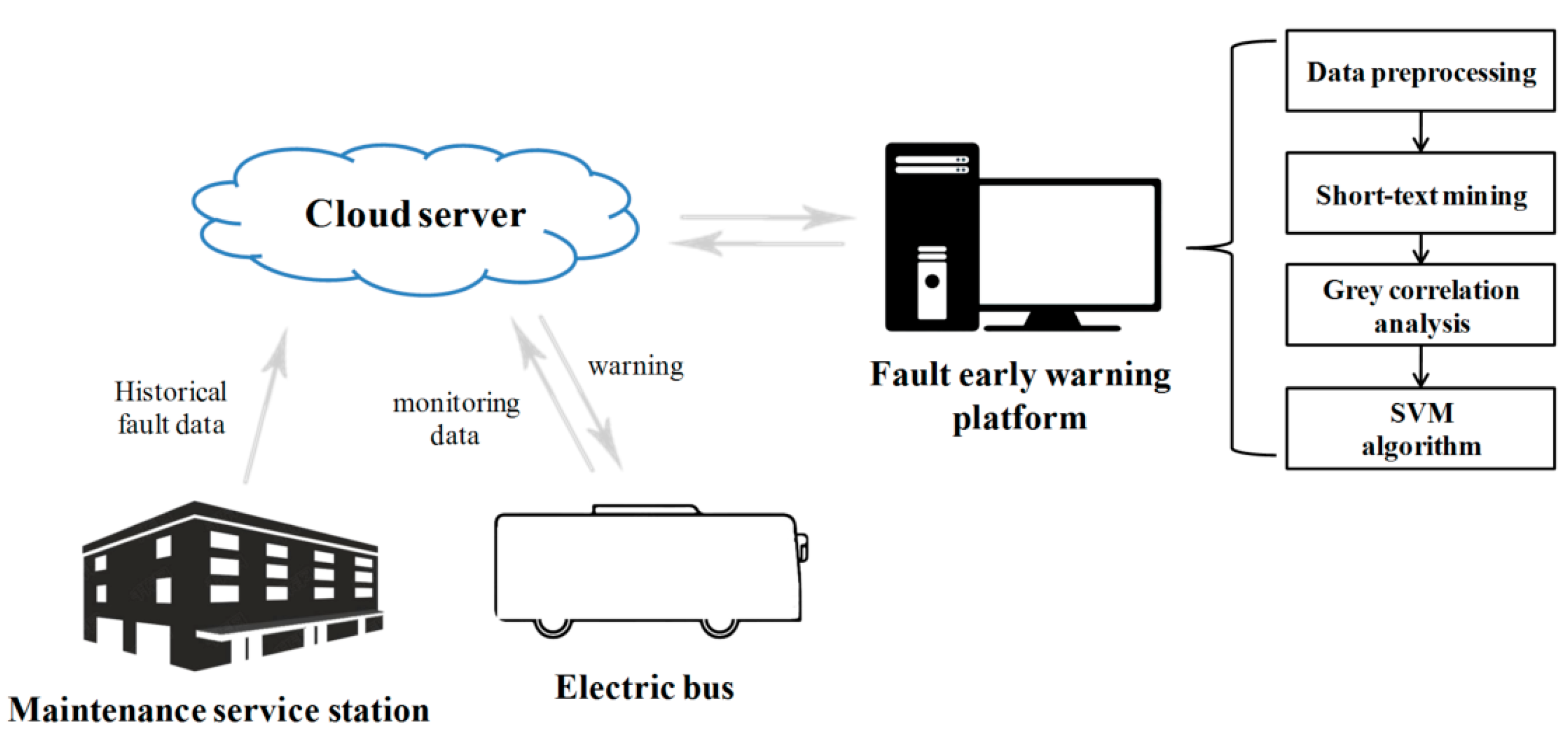
The crux of early fault warning lies in identifying the abnormal change in performance parameters. Once identified, the abnormality can consequently be determined to inform the users of the corresponding fault in the system. The architecture of the presented early fault warning scheme based on the fusion of short-text mining and the grey correlation is illustrated in Figure 1. It consists chiefly of the maintenance service station, electric bus, cloud server, and early fault warning platform. The monitoring data of the electric bus and the historical data recorded in the maintenance service station are forwarded to the cloud server to predict possible faults further. The early fault warning scheme is implemented in the platform, including data processing, short-text mining, the grey correlation analysis, and the support vector machine (SVM) algorithm.

Figure 1.
The architecture of early fault warning scheme.
2.1. Data Preprocessing
Even though the data forwarded to the cloud server are well sorted, various abnormal data still exist and will seriously impact further data mining and exploration. Therefore, it is necessary to conduct the data preprocessing most centered around the data cleansing, data integration, and data protocol application.
Data cleansing is the process of detecting and correcting (or removing) corrupt or inaccurate data [33]. The primary purpose of data cleansing is to improve data quality that can be preliminarily detected by the atlas. According to the theoretical correlation, the field data that have little impact on the research can be deleted. For the data with slow state change and a small number of vacancies, the interpolation mean method can be utilized in case of individual missing data, or the previous adjacent value can be adopted for replacement. In data cleansing, it is necessary to locate, find, and clean the adjacent problem data [34].
When integrating the data from different data sources, some data may be inconsistent and redundant, which will result in a poor prediction result and increasing time consumption. Based on the data protocol standard, it can adequately remove the redundant data, maintain the data consistency, and reduce the system complexity.
2.2. Short-Text Mining
The simple analysis of vehicle state data to predict the faults may lose the primary goal. Therefore, a fault prediction method of reliability statistics is adopted to find the name, time, and fault phenomenon of the key faults and to clarify the goal of the prediction model. The short-text mining method is applied to extract useful information from the unstructured text of various documents.
The text-mining process can be conducted as follows: the text contents are first preprocessed to extract the main features and then structured; later, the text can be decomposed and sorted by a related algorithm to obtain the required results. To reduce the computational difficulty, the sample text can be short-text-based. There are three steps in short-text mining, consisting of keyword extraction, key concept extraction, and topic description analysis. The keyword extraction is the main feature of text mining and the basis of the latter two works, which mainly use a mathematical tool to quantify and compare. Two main methods for keyword extraction are shown as follows:
- (1)
- Feature Selection Based on Statistical Words Occurrence Frequency: The occurrence frequency of keywords in the text is the key topic feature for analysis. The words occurring more often are retained, and the rest can be deleted to improve the accuracy of words in frequency screening. The term frequency-inverse document frequency (TF-IDF) algorithm is a relatively mature method for text mining, which can be defined with the calculation [35]:where is the occurrence frequency of the keyword in the sample text ; is the total number of keywords in the ; N is the total number of short texts in the training model; and is the number of texts containing keywords in the training model.
- (2)
- Information Gain: Based on the information entropy, this method is utilized to measure the proportion of a feature in classification and the amount of the information supplied. Concretely, it gauges the expected reduction in entropy [36]. The difference value between feature entropy can be introduced according to the amount of information:where is the occurrence probability of keyword category in the sample text; is the total number of keyword categories in the sample text; is the occurrence probability of keyword in the sample text; is the occurrence probability of keyword in the keyword category ; is the occurrence probability of keyword in the sample text; and is the occurrence probability of keyword category without keyword .
2.3. Grey Correlation Analysis
The grey correlation analysis is a general method to judge the correlation degree between various elements, which can be processed as follows [37]:
- (1)
- Determining the Sequence of Analysis: Two series should be determined in this step, including the reference series reflecting the feature of system behavior and the comparison series that can affect system behavior.The reference series can be formulated as:where is the kth variable in the initial sequence .The comparison series can be established as:where is the kth variable in .
- (2)
- Nondimensionalization of Variables: Given the data sequence , the mean change method can be employed. First, the average of each sequence can be calculated. Then, the average value with the data in the original sequence can be divided to generate a new data sequence. Last, the sequence average can be used to reflect the dynamic changes in the data.
- (3)
- Calculating the Difference Series, Extreme Value, and Grey Correlation Coefficient: Based on the dimensionless transformation, the related calculation can be obtained:where is the difference sequence; is the maximum value of ; is the minimum of ; is the grey correlation coefficient; and is the resolution coefficient.
- (4)
- Calculating the Correlation Value and Sorting: The correlation degree can be defined as the average value between the comparison series and the reference series:
2.4. SVM Algorithm
Fault prediction can be regarded as a binary classification problem. As a widely used supervised algorithm, the support vector machine (SVM) can provide uniqueness in the binary classification problem, for which the prediction accuracy and operational efficiency are pretty satisfactory [38].
In the SVM model, the sample set can be given as , where is the sample data, and is the output of the sample data. The equation is set as the classification line, where is the normal vector of the classification line, namely the vertical hyperplane. The position of the hyperplane can be adjusted by the parameter , where and are the problem solution [39]:
where is a positive scalar called the penalty coefficient, and is the slack variable for . Both and are hyperparameters.
When modifying the objective function, the Lagrange function can be introduced to solve the objective function, and the Lagrange multiplier is utilized to the constraints. Then, the original problem can be transformed into a computational dual optimization problem [40]:
SVM can be turned into a variety of completely different function models through different kernel functions . In this paper, different penalty factors are chosen to test and compare. By comparison, the solution with higher model prediction accuracy and lower model training time can be figured out.
2.5. Model Selection and Parameter Tuning for Machine Learning
SVM includes a key penalty factor and a variety of kernel functions. According to the characteristics of the key faults in electric buses, the test kernel functions selected in this study are the linear kernel function (Linear), Gaussian radial basis kernel function (RBF), polynomial kernel function (Poly), and Sigmoid kernel function (Sigmoid) for nonlinear action of neurons. These kernel functions share the same hyperparameter with the default value 1/k (k is the number of categories). In addition, the kernel function Poly has hyperparameters c and d, and the kernel function Sigmoid has a hyperparameter c that needs to be manually given and set, of which selection can refer to [41]. These two parameters also have system default values c = 0 and d = 3, which can be used in this work to compare the advantages and disadvantages of different kernel functions in the specified fault prediction preliminarily without setting hyperparameters.
Figure 2 provides a graphic explanation for model selection and parameter tuning, and the detailed descriptions are expressed as follows.
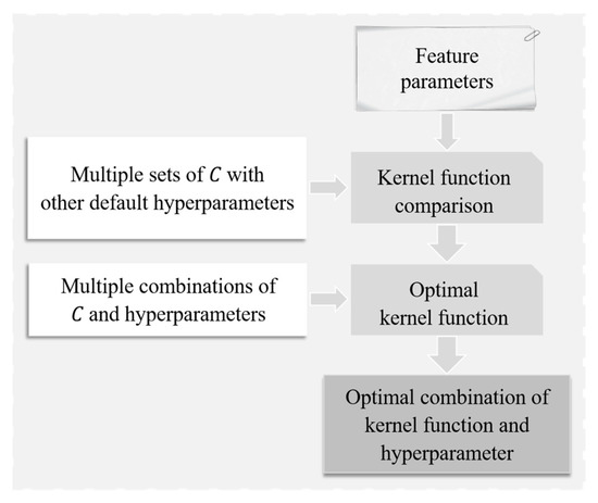
Figure 2.
The main flowchart of model selection and parameter tuning for machine learning.
Based on the default setting hyperparameters , c = 0, d = 3, only the key penalty factor will be changed first, and the key fault predictions of the four kernel functions in the same batch of electric buses will be compared. According to the prediction accuracy and the time-consuming performance of the model operation, the appropriate kernel function can be selected.
For further parameter tuning of the selected kernel functions, changing the value of the default hyperparameters and testing are necessary. The kernel function Linear has no additional hyperparameters, and it is only necessary to adjust the penalty factor further to find the most accurate and efficient model. The kernel function RBF has an additional hyperparameter , so it is necessary to adjust and concurrently, check the operation results for the parameters, analyze the relationship between different hyperparameter values and model effects, and find the most accurate and efficient model. The kernel function Poly needs to adjust the value of , , c, and d simultaneously, and the kernel function Sigmoid has to adjust the values of , , and c at the same time. After the comparison and analysis of different combinations of and other hyperparameters, the optimal model can then be selected.
3. Key Fault and Feature Parameter Extraction of Electric Buses
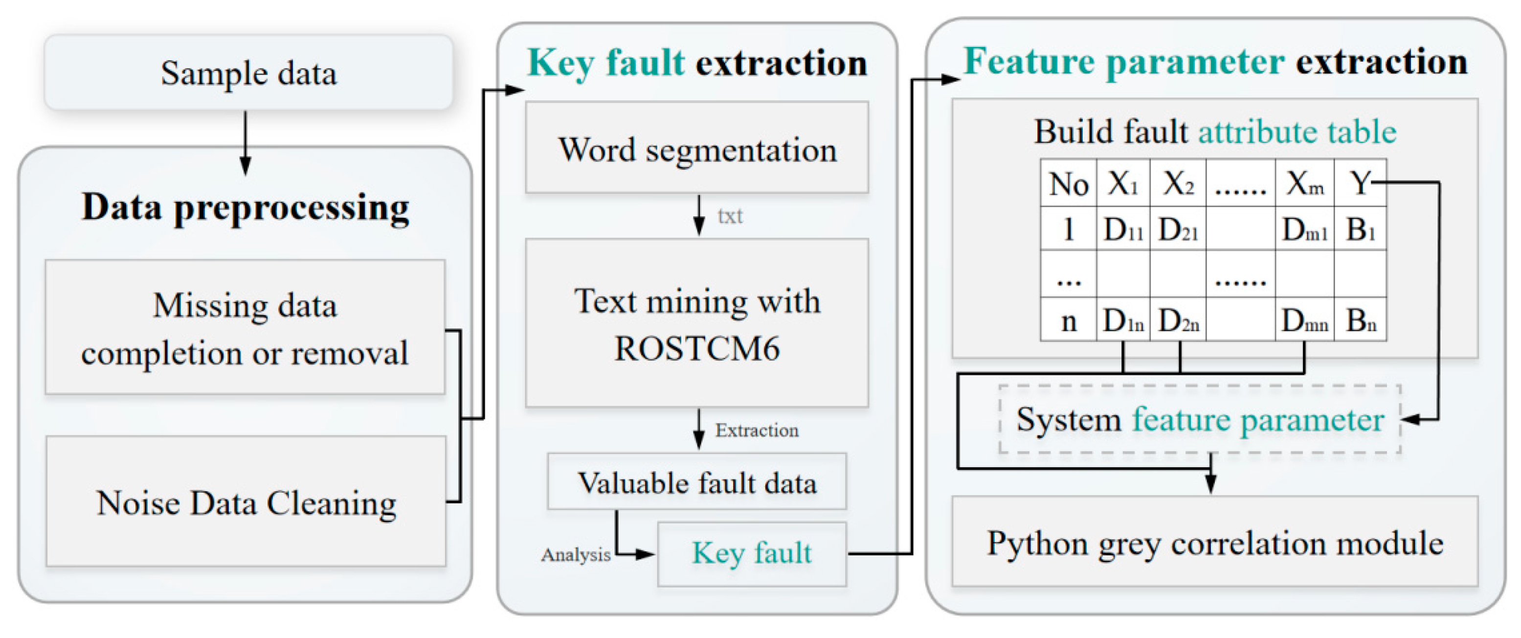
The sample data used in this study were taken in March 2021 from a batch of electric buses operating in Zhenjiang, China, produced in 2017. These data include vehicle maintenance data, alarm data, real-time monitoring bus state data, etc., which were stored in CAN or personnel filling documents. The data are applied to the scheme depicted in Section 2 to extract the key faults and feature parameters of electric buses, as described in Figure 3.
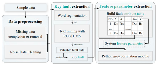
Figure 3.
The overall structure of key fault and feature parameter extraction.
3.1. Data Preprocessing
Since the data attributes and registration time are quite different, these data cannot be used directly. Data integration and preprocessing are necessary first.
After the vehicle data are transferred and stored, the following preprocessing can be carried out:
- (1)
- Missing Data Completion or Removal: Due to the inconsistency of the time axis of the intercepted data, the real-time state data of the vehicle may lose individual data. The data acquisition frequency is set as 10 s. Some data that change rapidly cannot be easily completed. Still, for data whose state does not change quickly, such as battery voltage and the state of charge (SOC), the interpolation mean method can be used for numerical substitution, or the last adjacent value can be used.
Firstly, vehicle data are extracted from the database according to the vehicle production serial number. Then, the content of the data field is analyzed by the atlas, and the quality of the field data is preliminarily detected. The list of fields that have little impact on the research can be deleted. If the value of a variable is missing a lot, but does not affect the research goal, the entire variable can be deleted.
- (2)
- Noise Data Cleaning: Noise data refer to erroneous data caused by system logic or information interference during acquisition. Noise data severely impact the results of later data processing, which need to be located first in data cleaning to find the adjacent problem data and remove it. Cleaning these noise data needs to be screened one by one according to the feature of electric buses and the correlation with the faults, and special tools are used for prevention and elimination.
3.2. Key Fault Extraction of Electric Buses Based on Short-Text Mining
In the actual vehicle maintenance and repair records, the content is filled in by the document-filling personnel of service stations or large group companies. The personnel who fill the report are generally not the actual maintenance personnel of the vehicle. They do not know the vehicle itself and only summarize and refine the “dictation” of the maintenance personnel and record it in the document. The document examiners who well master the vehicle knowledge can still comprehend the correct meaning when checking these incorrectly described words. However, the workload of order-by-order modification can be too large, and the economic benefits will be limited in the short term. Therefore, word segmentation should be performed on these spoken data. In word segmentation, the scattered data should be aggregated in the vehicle production serial number unit and converted into text format txt. to facilitate processing.
The txt. file can be analyzed by the ROSTCM6 text mining tool. The user data set can be loaded and processed according to the user’s needs and text characteristics. Load the special fault database data of new energy vehicles into the tool, and clear the records not in the user-defined package, such as prepositions, auxiliary words, faults in non-pure electric systems, etc. The number of original fault records used in the study is 580,000. After automatic word segmentation, the fault data can be reduced to 100,000, and the number of key fault items is 103. Finally, valuable fault information data are extracted for subsequent analysis. The top 10 key faults are listed as shown in Table 1.

Table 1.
Top 10 Key Faults and Word Frequency Analysis Results.
It can be clearly observed that “poor consistency of battery cells” is the main fault in electric buses due to the inconsistency of the production and use environment. Therefore, the feature parameters of this fault are further extracted in a follow-up study.
3.3. Feature Parameter Extraction Based on Grey Correlation Analysis
The grey correlation algorithm module is developed based on Python to normalize the vehicle state data, analyze the correlation degree between each vehicle state parameter and the decision factor “whether there is fault”, and calculate the correlation degree value. The main calculating process of the developed script is as follows:
- (1)
- Data normalization
- (2)
- Data standardization
- (3)
- Comparison with standard elements
- (4)
- Taking out the maximum and minimum values in the matrix
- (5)
- Calculation result
- (6)
- Calculating the mean value to obtain the grey correlation value
First, build the attribute table of the fault, and list each data item as a condition attribute. The result of whether the vehicle has faults is listed as the decision attribute. The fault state of electric buses is represented by “0” and “1” [42]; that is, “0” is used to indicate that the electric bus has “No failure”, and “1” is used to indicate “Failure”. The relevant parameters of the vehicle state and power battery state are selected as the influencing variables, denoted by X, where the total battery voltage of is X1; the total battery current is X2; the battery SOC is X3; the vehicle speed is X4; the travel of the accelerator pedal is X5; and the state of the brake pedal is X6. The situation after 1 h is the decision variable, expressed by Y. Then, the standardized data set can be obtained by dimensionless processing of the above data, as shown in Table 2.
Table 2.
Standardized Data Results of Grey Correlation Analysis.
According to the grey correlation analysis, the decision variable Y is used as the feature parameter of the system. Each attribute parameter is used as the sequence of the relevant factors for the failure “poor consistency of battery cells” to establish a sub-sequence and solve it in the Python model to obtain the result shown in Table 3.
Table 3.
Grey Correlation Analysis Results.
According to Table 3, the grey correlation degree is sorted from large to small, and the order is that the total battery current X2 > the total battery voltage X1 > the battery SOC X3 > the travel of accelerator pedal X5 > the state of brake pedal X6 > the speed of electric bus X4. Generally, when the grey correlation degree is greater than 0.5, it indicates that the parameter has a greater impact on the system and should be paid special attention to. Combined with the calculation results of the grey correlation degree, the state data of the battery itself has a relatively large correlation to the occurrence of “poor consistency of battery cells”. At the same time, the correlation degree of the three parameters in the vehicle state attributes is between 0.45 and 0.5, which is relatively large, indicating that the correlation between each system and the occurrence of fault in the initial stage is consistent with the result of data analysis.
4. Results and Discussion of Early Fault Warning Based on SVM
In this section, a prediction model is obtained for early fault warning of batteries, of which the effectiveness is verified. The establishment of the prediction model based on SVM can be generally divided into two steps: kernel function selection and hyperparameter tuning.
4.1. Kernel Function Selection
Using the sklearn module in the Python scripting tool, a comparison module for different kernel functions can be built. To facilitate manual parameter adjustment, only one value of the penalty factor C is used in each test. The next value of C can be adjusted according to the tested results. The designed Python script operation process is as follows:
- (1)
- Read the data and divide it into the training set and test set.
- (2)
- Set the penalty factor C; evaluate the training accuracy and the computing efficiency of the model.
- (3)
- Visualize the model results and guide to set the next value of C.
Each time a penalty factor C value is set for the test, the test results are recorded, and the results of multiple tests are compared to obtain a proper model. After testing, the value of the penalty factor C is chosen to be {0.1, 0.5, 1, 3, 5, 15, 30, 50}, and the performance of four kernel functions with the same value C is compared.
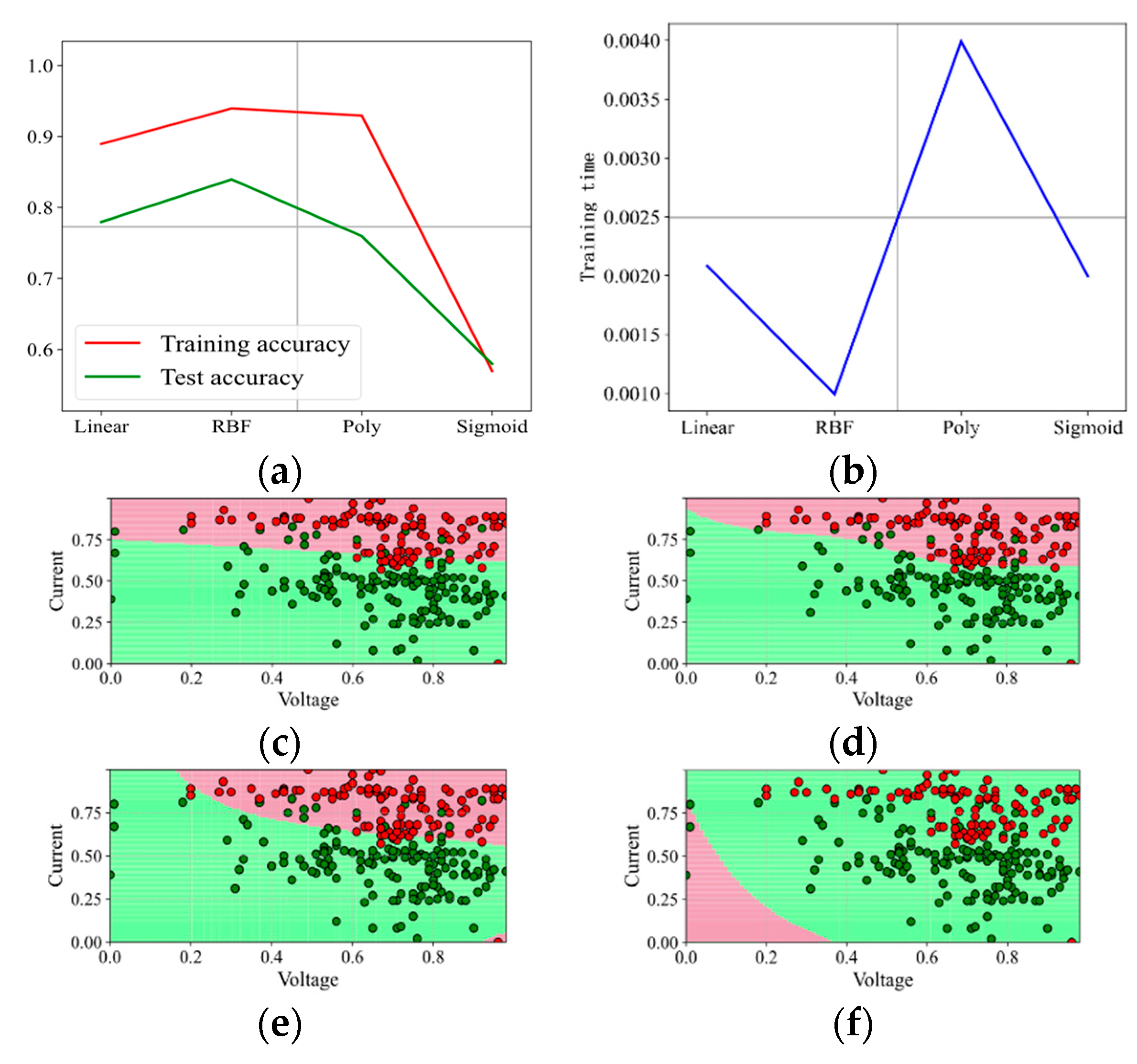
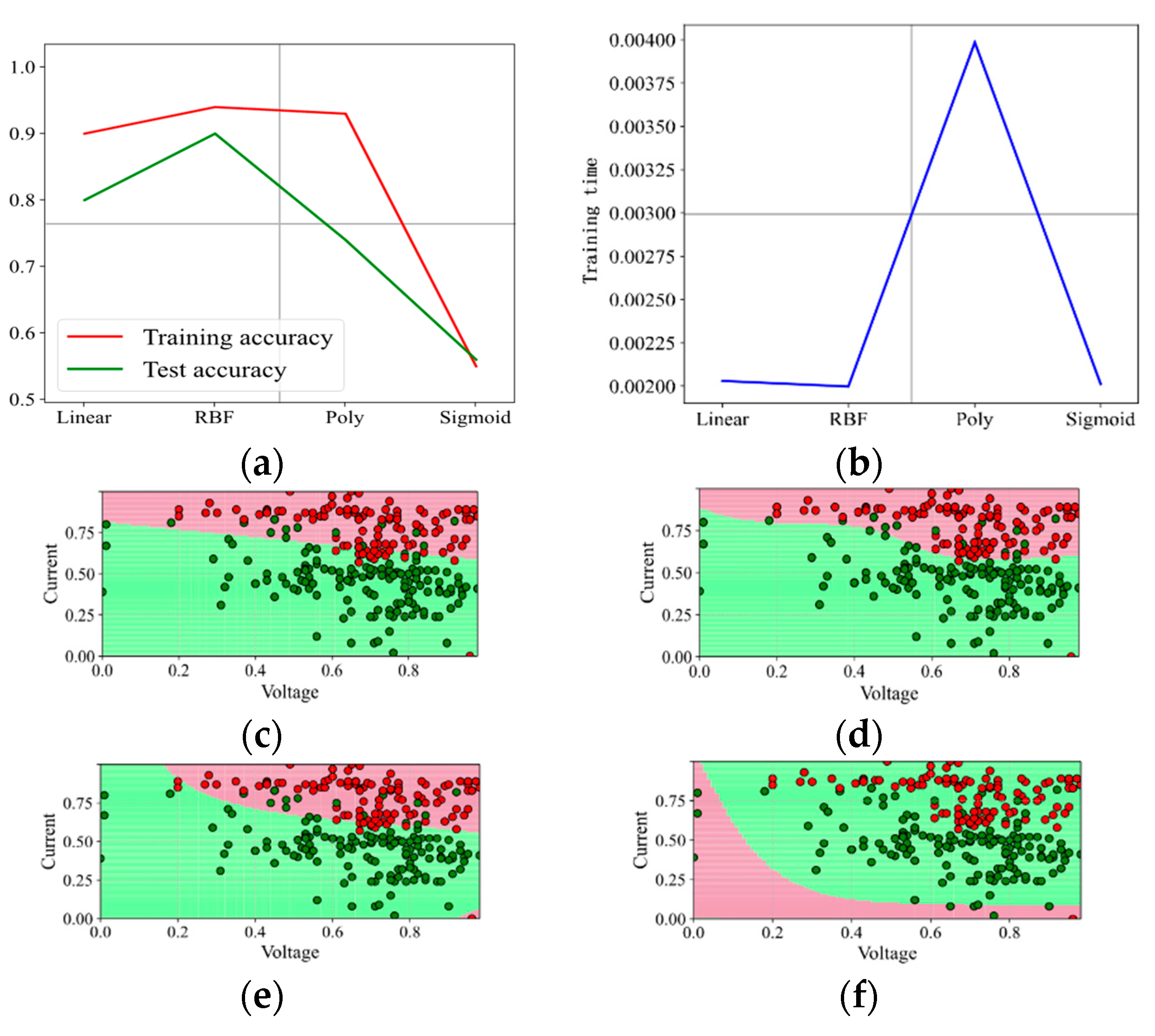
When the penalty factor C is 0.1, the prediction results are shown in Figure 4. The kernel function Poly has the highest training accuracy under the data set and penalty factor, reaching 93%, but the test accuracy is only 76%, and the training time is longer than other kernel functions; the test accuracy of the kernel function Linear and RBF is 78%; RBF is better in training accuracy, but the training time is longer; the overall prediction effect of the kernel function Sigmoid is the worst; the training accuracy and test accuracy are only 58%, and the training time is up to 2 ms. It can also be seen from the binary effect diagram that the kernel function Sigmoid does not correctly separate the “red faulty vehicle” from the “green non-faulty vehicle”, which performs the worst. In this round of test, the kernel functions RBF and Poly distinguish the “red faulty vehicle” from the “green non-faulty vehicle” accurately. The effect of the kernel function Linear is not good.
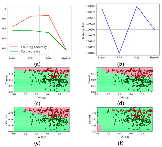
Figure 4.
Prediction effect with penalty factor C = 0.1. (a) Model prediction accuracy. (b) Model training time. (c) Prediction effect with kernel function Linear. (d) Prediction effect with kernel function RBF. (e) Prediction effect with kernel function Poly. (f) Prediction effect with kernel function Sigmoid.
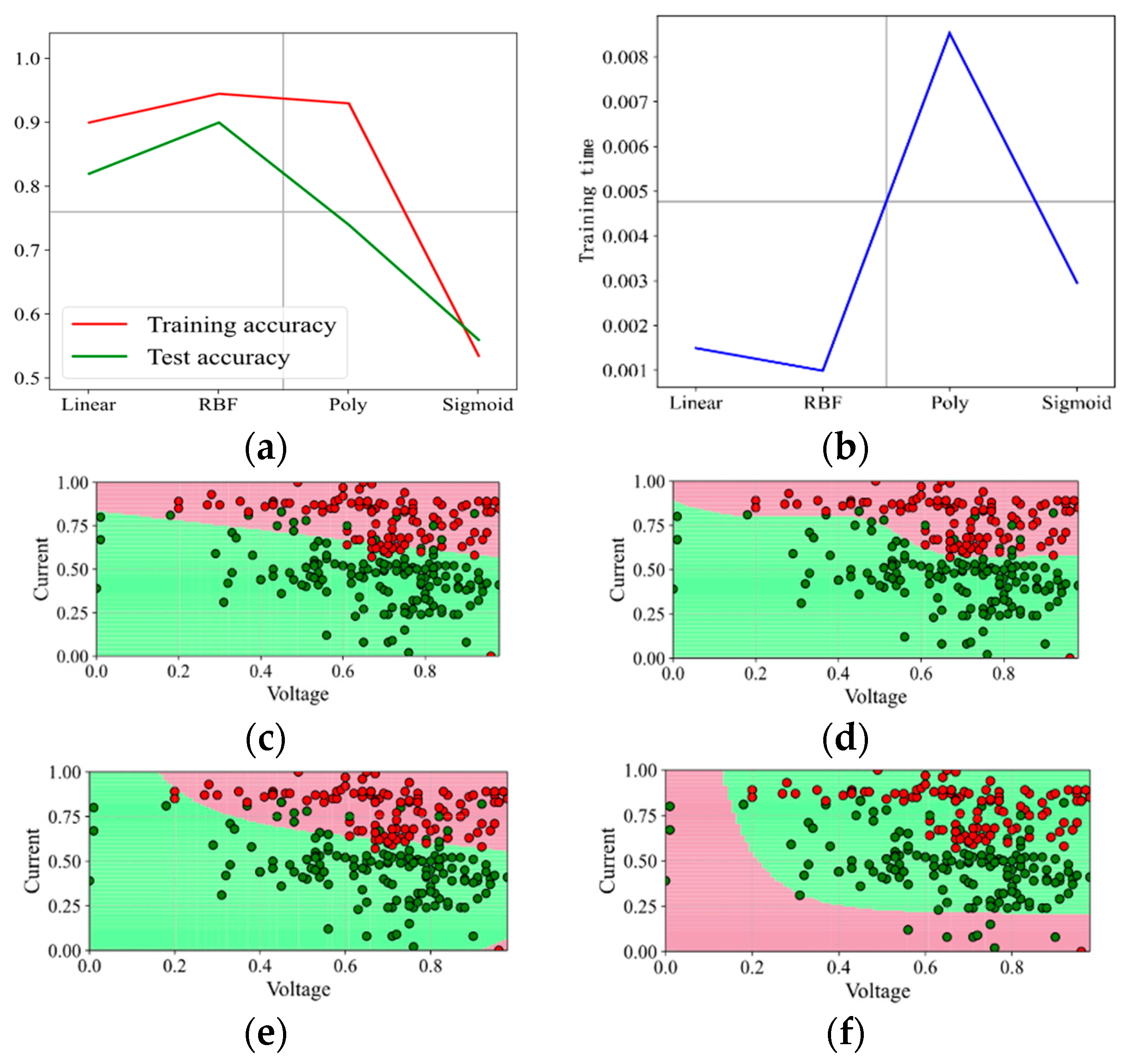
Figure 5 shows the prediction accuracy, training time, and prediction effect of the four kernel functions when the penalty factor C = 0.5. With the increase in C, the overall prediction effect is consistent when C = 0.1, and the comparison of the four kernel functions changes slightly. According to Figure 4 and Figure 5, the kernel function Sigmoid is not suitable for the binary analysis of the data set. The kernel functions Linear, RBF, and Poly perform well. At the same time, with the increase in the penalty factor C, the effect is improved. The kernel function RBF enhances the effect most and takes the least time.
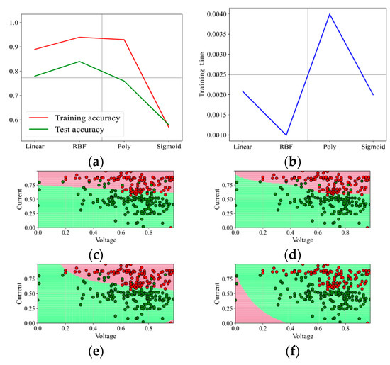
Figure 5.
Prediction effect with penalty factor C = 0.5. (a) Model prediction accuracy. (b) Model training time. (c) Prediction effect with kernel function Linear. (d) Prediction effect with kernel function RBF. (e) Prediction effect with kernel function Poly. (f) Prediction effect with kernel function Sigmoid.
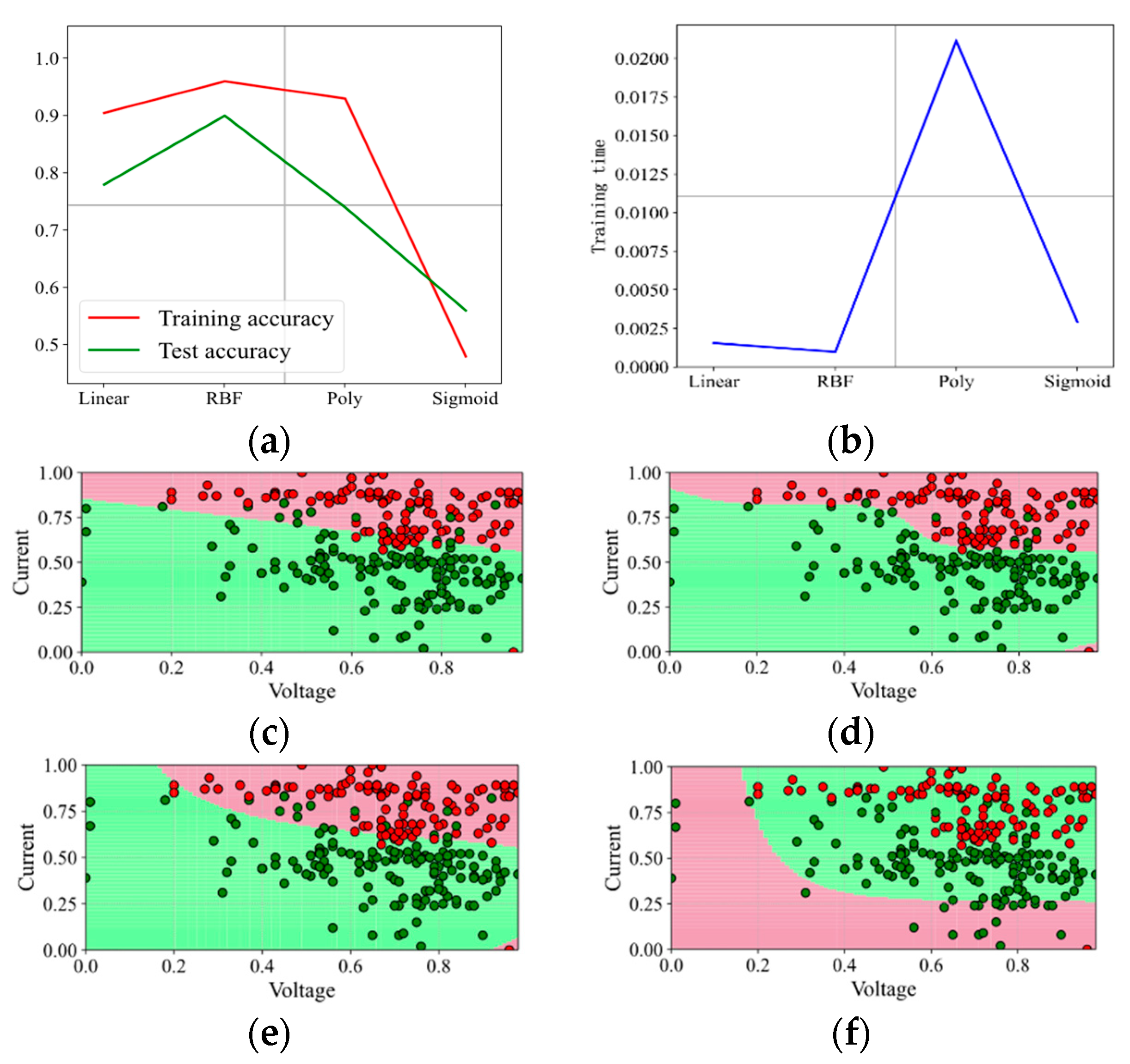
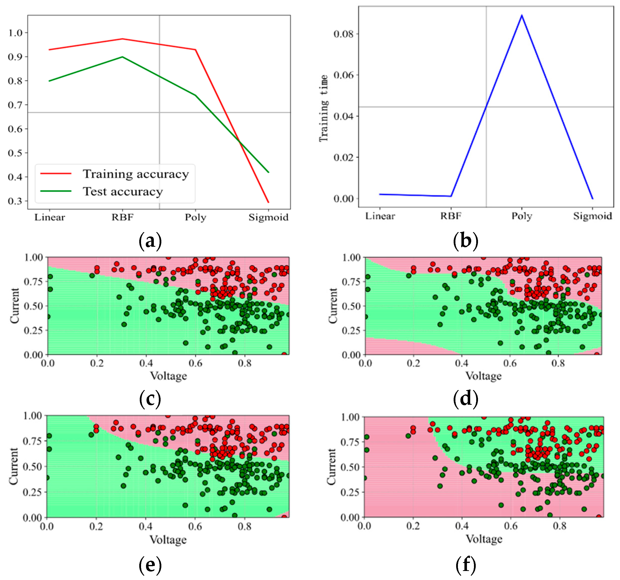
With increasing the penalty factor C, the effect when C is set as 1 and 3 is shown in Figure 6 and Figure 7. With the continuous increase in C, the prediction effect is also improving. With C increasing up to 5 and even 50, the effect is shown in Figure 8 and Figure 9. It shows that when the penalty factor C increases up to 50, the increase in C has little effect on the effect of kernel functions RBF and Poly, and the training time increases slightly.
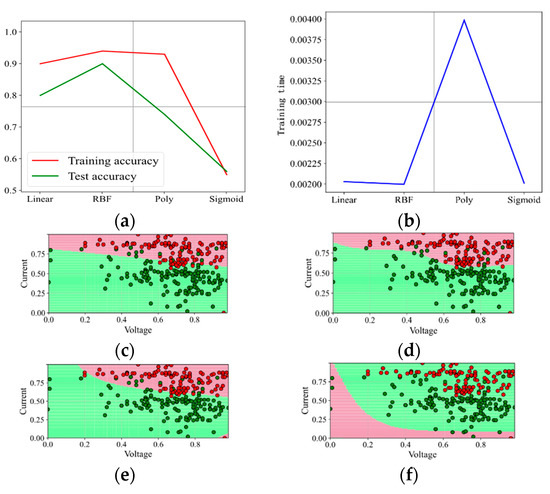
Figure 6.
Prediction effect with penalty factor C = 1. (a) Model prediction accuracy. (b) Model training time. (c) Prediction effect with kernel function Linear. (d) Prediction effect with kernel function RBF. (e) Prediction effect with kernel function Poly. (f) Prediction effect with kernel function Sigmoid.

Figure 7.
Prediction effect with penalty factor C = 3. (a) Model prediction accuracy. (b) Model training time. (c) Prediction effect with kernel function Linear. (d) Prediction effect with kernel function RBF. (e) Prediction effect with kernel function Poly. (f) Prediction effect with kernel function Sigmoid.
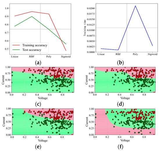
Figure 8.
Prediction effect with penalty factor C = 5. (a) Model prediction accuracy. (b) Model training time. (c) Prediction effect with kernel function Linear. (d) Prediction effect with kernel function RBF. (e) Prediction effect with kernel function Poly. (f) Prediction effect with kernel function Sigmoid.
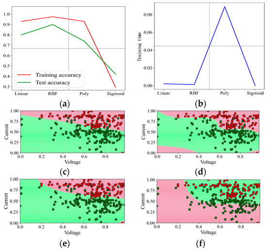
Figure 9.
Prediction effect with penalty factor C = 50. (a) Model prediction accuracy. (b) Model training time. (c) Prediction effect with kernel function Linear. (d) Prediction effect with kernel function RBF. (e) Prediction effect with kernel function Poly. (f) Prediction effect with kernel function Sigmoid.
According to the test results and analysis, it can be concluded that the kernel function RBF is more suitable for the fault prediction of “poor consistency of battery cells”.
4.2. Tuning Hyperparameters of the Kernel Function RBF
The sklearn module in the Python scripting tool is used to establish the comparison module of the selected kernel function RBF under different hyperparameters. In each test, only one value of the penalty factor C is used, and a different hyperparameter is set for testing at the same time. In the study, six groups of are tested under the same value of the penalty factor C. Then, the next value C will be selected to compare the tested results.
The designed Python script operation process is as follows:
- (1)
- Reading the data and dividing it into the training set and test set.
- (2)
- Setting the penalty factor C and passing it to six models with different hyperparameters respectively.
- (3)
- Model training.
- (4)
- Evaluating the effect of accuracy and operation efficiency of the model.
- (5)
- Visualizing the model results and setting the next value C.
- (6)
- Repeating the above operations until the model effect is stable and finding a suitable combination of penalty factor C and hyperparameter .
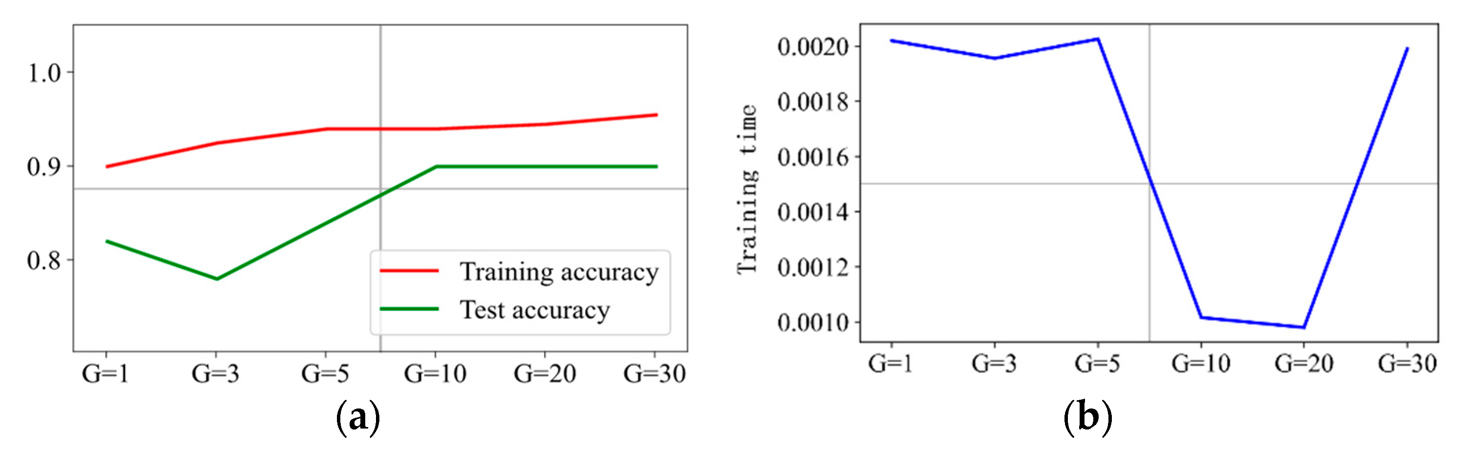
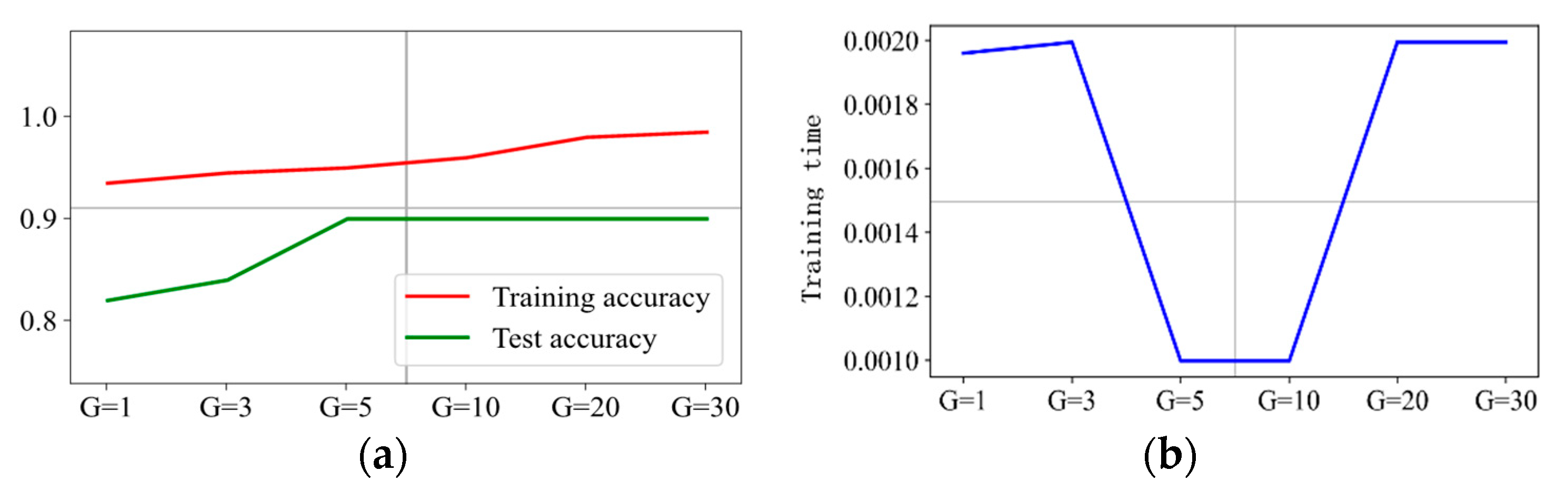
According to the above-depicted research, the value of the penalty factor C is selected as {1, 3, 5, 10, 20, 30}, and the kernel function RBF has another hyperparameter . Combined with the experiment test, the value of the hyperparameter is selected to be {1, 3, 5, 10, 20, 30} as well. Six values of {1, 3, 5, 10, 20, 30} are taken to test for each penalty factor C and to compare. When the penalty factor C is 1 and 3, the results of six groups of are shown in Figure 10 and Figure 11.
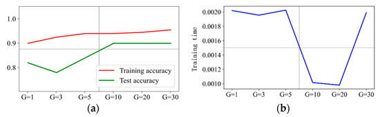
Figure 10.
Prediction effect with penalty factor C = 1. (a) Model prediction accuracy. (b) Model training time.
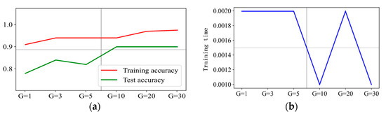
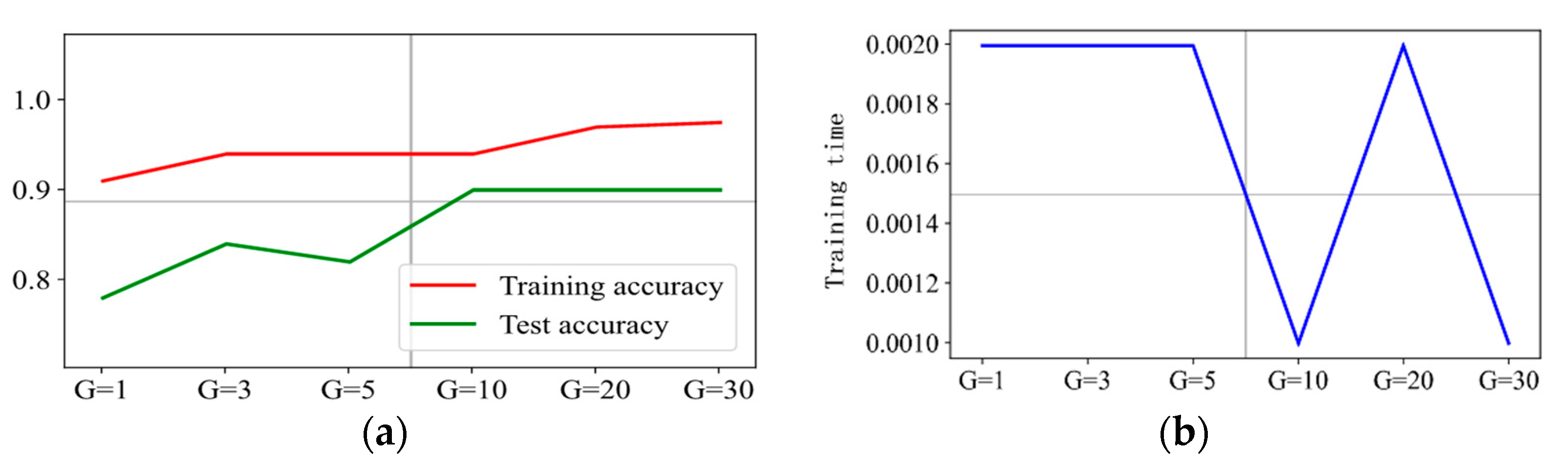
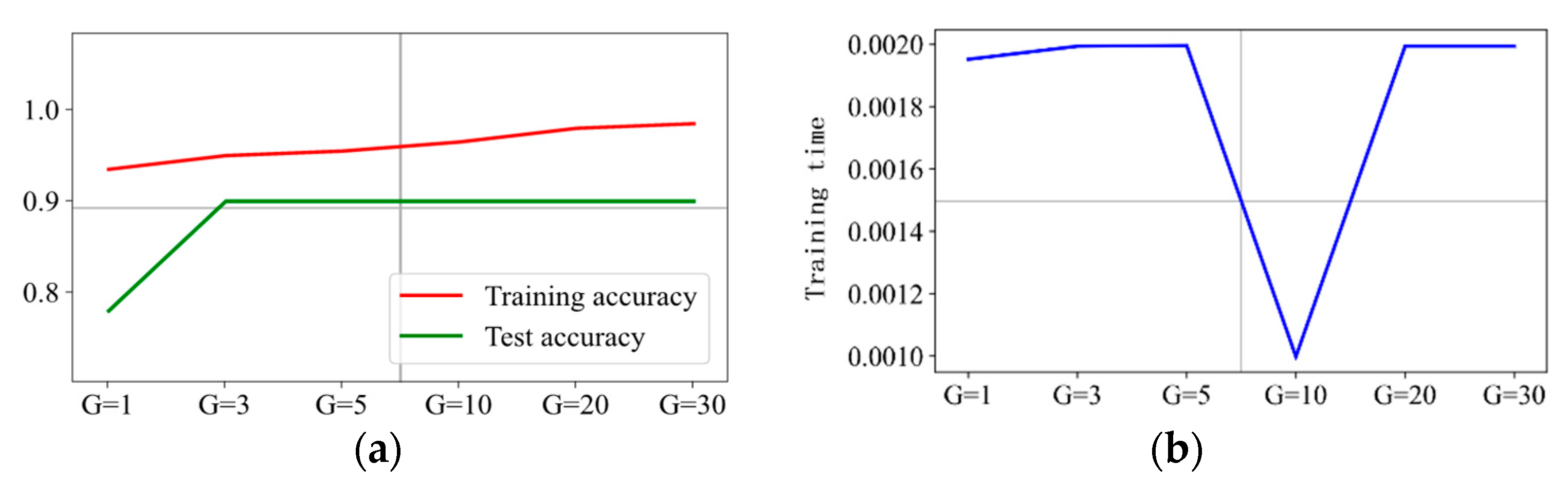
Figure 11.
Prediction effect with penalty factor C = 3. (a) Model prediction accuracy. (b) Model training time.
Figure 10 shows the prediction accuracy, training time, and prediction effect of six groups of with penalty factor C = 1. It shows that the training accuracy increases from 92% with to 97% with , but the training accuracy does not increase anymore when the value of further increased. The overall change trend of test accuracy also increases from 78% when to 90% when . However, the test accuracy does not increase anymore when the value of is further increased. The training time is 2 ms when , and as the value of increases, the training time is kept around 1.2 ms. In addition, there is a flection point, which is 2.1 ms when . Therefore, we can conclude that is the optimal hyperparameter when the penalty factor C = 1. Figure 11 shows the results with six groups of when the penalty factor C = 3. It can be observed that the prediction accuracy and training time have similar change trends to those when C = 1, and it can be concluded that is the optimal hyperparameter for penalty factor C = 3.
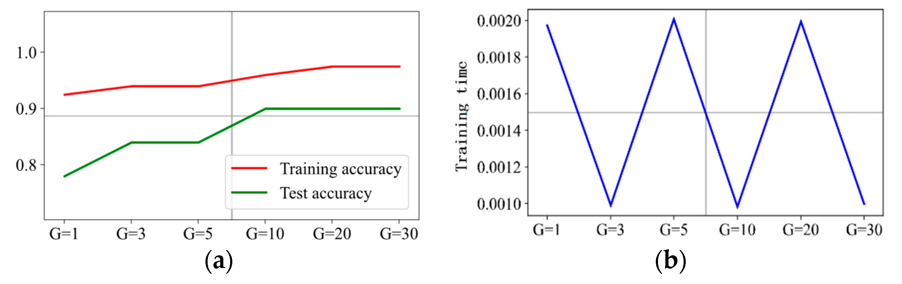
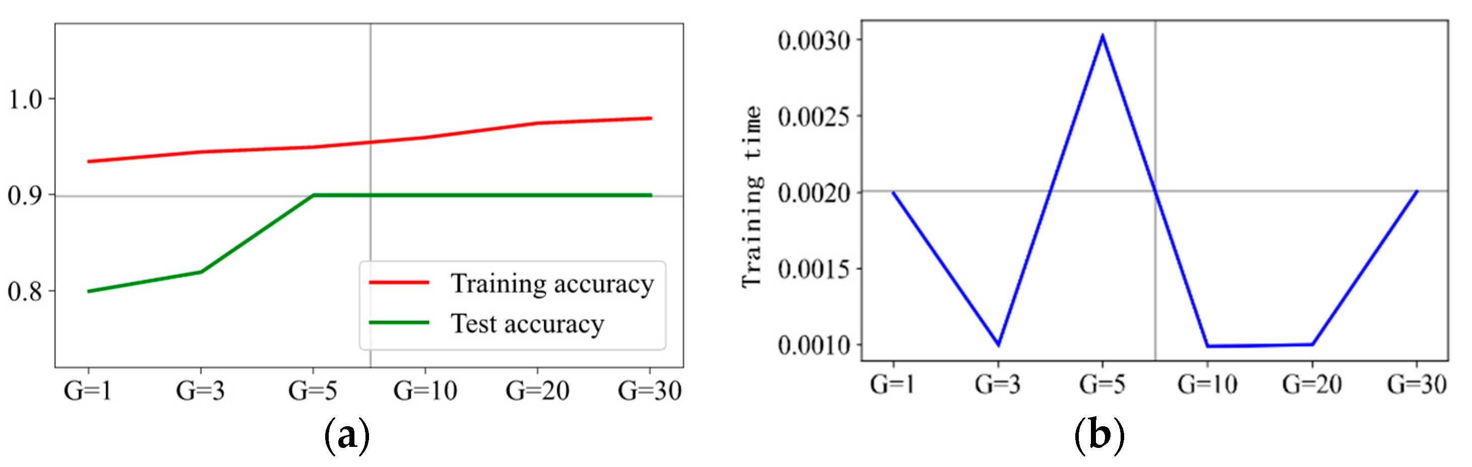
The prediction results are presented in Figure 12, Figure 13, Figure 14 and Figure 15 when C is 5, 10, 20, and 30, respectively. It can be concluded that is the optimal hyperparameter for penalty factor C = 5, and is the optimal one for penalty factor C = 10, 20, and 30.

Figure 12.
Prediction effect with penalty factor C = 5. (a) Model prediction accuracy. (b) Model training time.
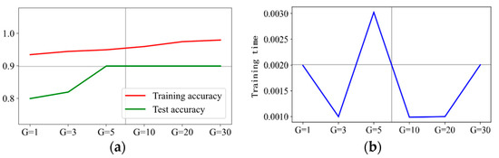
Figure 13.
Prediction effect with penalty factor C = 10. (a) Model prediction accuracy. (b) Model training time.
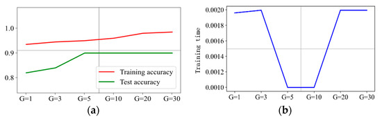
Figure 14.
Prediction effect with penalty factor C = 20. (a) Model prediction accuracy. (b) Model training time.
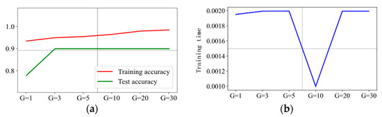
Figure 15.
Prediction effect with penalty factor C = 30. (a) Model prediction accuracy. (b) Model training time.
According to the above test results, we can conclude that the kernel function RBF is the most suitable for the fault data set “poor consistency of battery cells”, and the kernel function RBF with penalty factor C = 3 and hyperparametric is the optimized model for predicting the specified faulty. It has the advantages in curve fitting, test set accuracy, and model training time.
4.3. Experimental Verification
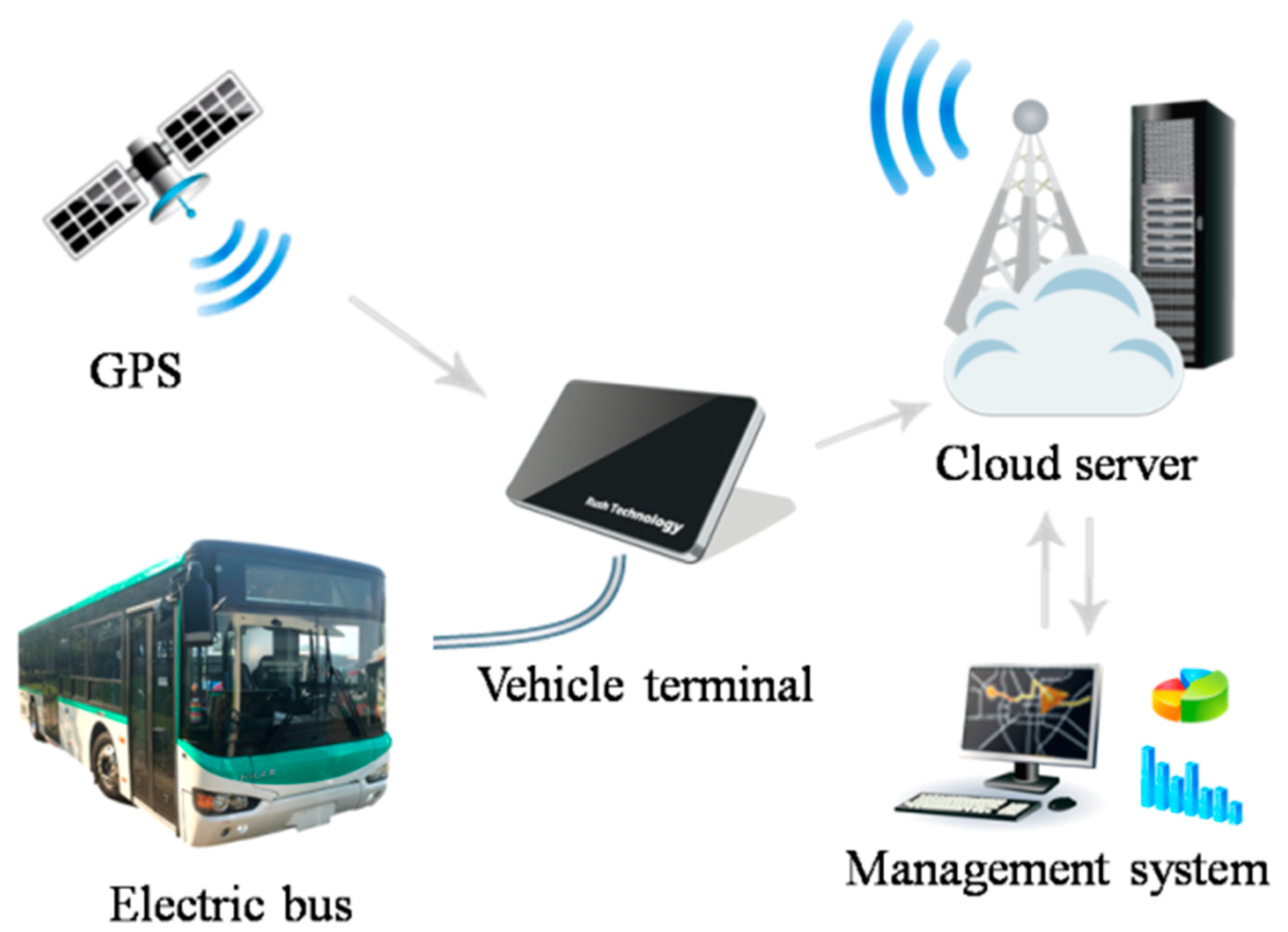
To verify the effectiveness of the key fault prediction model, the data of the same batch of electric buses are selected for verification, with a test system from the Higer Bus Company shown in Figure 16. The test system consists of the electric buses, vehicle terminal, cloud server, and management system. The battery state data of electric buses are transmitted to the cloud server through the vehicle terminal, and the cloud server transmits the data to the management system to implement the experimental operation.
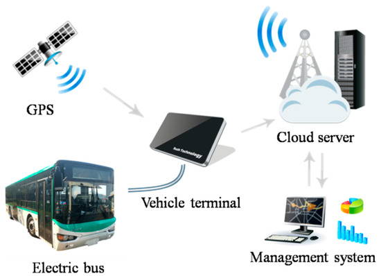
Figure 16.
A test system for key early fault warning method of electric buses from Higer Bus Company Limited.
For the model evaluation of the binary classification problem, since the actual fault probability of the vehicle is small, and the vehicle fault after one hour corresponding to most of the vehicle state data is “No fault”, the best verification method for this situation is to use the confusion matrix [43]. The specific operation of the verification method is as follows:
- (1)
- Extract the state parameters of some faulty electric buses one hour before the fault to form a real vehicle fault data set.
- (2)
- Input the fault data set into the model for calculation, record the results of early fault warning, and fill the data with the correct prediction and wrong prediction into the confusion matrix.
- (3)
- Extract the state parameters of some non-faulty electric buses to form a real vehicle fault-free data set.
- (4)
- Input the fault-free data set into the model for calculation, record the results of early fault warning, and fill the data with the correct prediction and wrong prediction into the confusion matrix.
- (5)
- Calculate the data in the confusion matrix, obtain the harmonic average value, and determine the prediction accuracy.
As above-mentioned, the data used to build the model and tune the model parameters were taken in March 2021 from a batch of electric buses operating in Zhenjiang. The vehicle state and the fault data of the same batch of electric buses in April 2021 were used for verification in this test. Select the kernel function RBF in SVM with the penalty factor C = 3 and hyperparameter . The confusion matrix of fault prediction results is shown in Table 4. The average harmonic value of the fault prediction is 85.2%, which shows that the model can meet the faulty prediction expectations.
Table 4.
The Confusion Matrix of a Batch of Electric Buses’ Fault Prediction Results.
5. Conclusions
This paper presents a data-driven early fault warning method that combines the advantages of reliability statistics and information processing based on big data analysis. Through short-text mining, the fault information recorded in various vehicle maintenance and service documents is identified, and the key fault types and names of electric buses are statistically analyzed. Through the grey correlation algorithm, the monitoring bus state data are processed. By processing and analysis, the key feature variables related to failures are extracted. The values of key feature variables in the vehicle state one hour before the failure are extracted to establish a machine learning model and predict the faulty possibility of vehicles in the next coming hour. Based on the SVM algorithm, the process of prediction model establishment and evaluation indicators are discussed. First, only the value of the penalty factor C is adjusted to find the proper kernel function with higher accuracy and lower operation time in fault prediction by comparing the effects of various kernel functions. Then, through the establishment of the data test matrix, the penalty factor C and the value of the other hyperparameters are adjusted simultaneously to obtain the optimized model. Finally, the fault prediction model is verified by comparing the predicted result with further obtained real fault data of electric buses. The results show that the key fault prediction model of electric buses based on big data can effectively predict the vehicle faults and carry out the early fault warning.
It should be mentioned that the described scheme is a data-driven method, which provides high performance for prediction; however, it still depends on the volume of data. The results might be inaccurate when applying to a limited data set. Moreover, further improvement of prediction performance can be offered by developing the presented method. In future work, it is necessary to consider distinguishing and effective clustering of vehicles in different states and then carry out the data-driven fault prediction, which can improve the effectiveness of the model prediction. In addition, the analysis process can be further optimized. The analysis system can process the data and model adjustment by itself to improve the reliability of the prediction model further and reduce the application cost.
Author Contributions
Conceptualization, Z.Z. and J.N.; methodology, Z.Z. and J.N.; software, Z.Z. and B.D.; validation, B.D., Z.Z. and J.N.; formal analysis, B.D. and Z.Z.; investigation, Z.Z. and B.D.; resources, J.N.; data curation, Z.Z. and B.D.; writing—original draft preparation; B.D., Y.C. (Yili Cai) and Z.Z.; writing—review and editing, B.D., W.C., Y.C. (Yuhua Chang) and J.H.; visualization, Z.Z. and B.D.; supervision, J.N., W.C., Y.C. (Yuhua Chang) and J.H.; funding acquisition, J.N. and W.C. All authors have read and agreed to the published version of the manuscript.
Funding
This research was funded by the National Key Research and Development Program of China, grant number 2020YFB1600203.
Institutional Review Board Statement
Not applicable.
Informed Consent Statement
Not applicable.
Data Availability Statement
Not applicable.
Conflicts of Interest
The authors declare no conflict of interest.
References
- Zhao, Y.; Wang, Z.; Shen, Z.; Sun, F. Data-driven framework for large-scale prediction of charging energy in electric vehicles. Appl. Energy 2021, 282, 116175. [Google Scholar] [CrossRef]
- Sun, Z.; Han, Y.; Wang, Z.; Chen, Y.; Liu, P.; Qin, Z.; Song, C. Detection of voltage fault in the battery system of electric vehicles using statistical analysis. Appl. Energy 2022, 307, 118172. [Google Scholar] [CrossRef]
- Si, J.; Ma, J.; Niu, J.; Wang, E. An intelligent fault diagnosis expert system based on fuzzy neural network. J. Vib. Shock 2017, 36, 164–171. [Google Scholar]
- Xu, Z. Leakage prediction of swing cylinder in concrete pump truck based on the improved direct grey model. J. Wuhan Univ. Sci. Technol. (Nat. Sci. Ed.) 2015, 6, 459–462. [Google Scholar]
- Li, J. Research on Safety Evaluation Method and Application of Vehicle Running State. Master’s Thesis, Beijing Jiaotong University, Beijing, China, 2007. [Google Scholar]
- Hao, X. Wang Yunsong, deputy director of the Quality Development Bureau of the State Market Supervision Administration: The recall of cars in 2021 mainly focused on electronic and electrical appliances, engines and other assemblies. Prod. Reliab. Rep. 2022, 1, 65–66. [Google Scholar]
- Jiang, X.; Fu, X.; Yang, Z. Application of RBF neural network method in remote monitoring system for vehicle state. Automob. Technol. 2011, 3, 23–26. [Google Scholar]
- Wu, J.; Song, L.; Chen, J. Common faults and treatment of bus CAN bus. People’s Public Transp. 2012, 2, 64. [Google Scholar] [CrossRef]
- Zeng, S.; Pecht, M.; Wu, J. Status and perspectives of prognostics and health management technologies. Acta Aeronaut. Astronaut. Sin. 2005, 26, 626–632. [Google Scholar]
- Zhai, H.; Xue, L.; Pei, D. Investigation and statistical analysis of the distribution characteristics of bus fault. Automob. Technol. 2017, 2, 208–210. [Google Scholar]
- Chen, F. Research classification algorithm based on support vector machine. Comput. Netw. 2009, 35, 64–67. [Google Scholar]
- Xuan, R. Vehicle Health Management and Monitoring System Based on Big Data. Master’s Thesis, Southeast University, Nanjing, China, 2017. [Google Scholar]
- Yılmaz, A.; Bayrak, G. A new signal processing-based islanding detection method using pyramidal algorithm with undecimated wavelet transform for distributed generators of hydrogen energy. Int. J. Hydrogen Energy 2022, 47, 19821–19836. [Google Scholar] [CrossRef]
- Patil, A.; Mishra, B.; Harsha, S. A mechanics and signal processing based approach for estimating the size of spall in rolling element bearing. Eur. J. Mech. A/Solids 2021, 85, 104125. [Google Scholar] [CrossRef]
- Hanna, S.; Dick, C.; Cabric, D. Signal Processing-Based Deep Learning for Blind Symbol Decoding and Modulation Classification. IEEE J. Sel. Areas Commun. 2021, 40, 82–96. [Google Scholar] [CrossRef]
- Ma, M.; Wang, Y.; Duan, Q.; Wu, T.; Sun, J.; Wang, Q. Fault detection of the connection of lithium-ion power batteries in series for electric vehicles based on statistical analysis. Energy 2018, 164, 745–756. [Google Scholar] [CrossRef]
- Rubini, R.; Meneghetti, U. Application of the envelope and wavelet transform analyses for the diagnosis of incipient faults in ball bearings. Mech. Syst. Signal Processing 2001, 15, 287–302. [Google Scholar] [CrossRef]
- Cheng, J.; Yu, D.; Yang, Y. Application of an impulse response wavelet to fault diagnosis of rolling bearings. Mech. Syst. Signal Processing 2007, 21, 920–929. [Google Scholar] [CrossRef]
- Fadaei, A.; Khasteh, S. Enhanced K-means re-clustering over dynamic networks. Expert Syst. Appl. 2019, 132, 126–140. [Google Scholar] [CrossRef]
- Fränti, P.; Sieranoja, S. How much can k-means be improved by using better initialization and repeats? Pattern Recognit. 2019, 93, 95–112. [Google Scholar] [CrossRef]
- Yang, R.; Xiong, R.; Ma, S.; Lin, X. Characterization of external short circuit faults in electric vehicle Li-ion battery packs and prediction using artificial neural networks. Appl. Energy 2020, 260, 114253. [Google Scholar] [CrossRef]
- Lee, S.; Han, S.; Han, K.; Kim, Y.; Agarwal, S.; Hariharan, K.; Oh, B.; Yoon, J. Diagnosing various failures of lithium-ion batteries using artificial neural network enhanced by likelihood mapping. J. Energy Storage 2021, 40, 102768. [Google Scholar] [CrossRef]
- Wang, P.; Zhang, J.; Wan, J.; Wu, S. A fault diagnosis method for small pressurized water reactors based on long short-term memory networks. Energy 2022, 239, 122298. [Google Scholar] [CrossRef]
- Kapucu, C.; Cubukcu, M. A supervised ensemble learning method for fault diagnosis in photovoltaic strings. Energy 2021, 227, 120463. [Google Scholar] [CrossRef]
- Zhang, Z. Research on Fault Early Warning Based on Big Data Mining. Master’s Thesis, Beijing University of Posts and Telecommunications, Beijing, China, 2018. [Google Scholar]
- Nan, J.; Deng, B.; Cao, W.; Tan, Z. Prediction for the Remaining Useful Life of Lithium–Ion Battery Based on RVM-GM with Dynamic Size of Moving Window. World Electr. Veh. J. 2022, 13, 25. [Google Scholar] [CrossRef]
- Ji, C.; Sun, W. A review on data-driven process monitoring methods: Characterization and mining of industrial data. Processes 2022, 10, 335. [Google Scholar] [CrossRef]
- Dina, N.; Yunardi, R.; Firdaus, A. Utilizing Text Mining and Feature-Sentiment-Pairs to Support Data-Driven Design Automation Massive Open Online Course. Int. J. Emerg. Technol. Learn. (iJET) 2021, 16, 134–151. [Google Scholar] [CrossRef]
- Xu, H.; Liu, Y.; Shu, C.; Bai, M.; Motalifu, M.; He, Z.; Wu, S.; Zhou, P.; Li, B. Cause analysis of hot work accidents based on text mining and deep learning. J. Loss Prev. Process Ind. 2022, 76, 104747. [Google Scholar] [CrossRef]
- Schmid, M.; Kneidinger, H.; Endisch, C. Data-driven fault diagnosis in battery systems through cross-cell monitoring. IEEE Sens. J. 2020, 21, 1829–1837. [Google Scholar] [CrossRef]
- Zhang, K.; Hu, X.; Liu, Y.; Lin, X.; Liu, W. Multi-fault Detection and Isolation for Lithium-Ion Battery Systems. IEEE Trans. Power Electron. 2021, 37, 971–989. [Google Scholar] [CrossRef]
- Zhao, Y.; Liu, P.; Wang, Z.; Zhang, L.; Hong, J. Fault and defect diagnosis of battery for electric vehicles based on big data analysis methods. Appl. Energy 2017, 207, 354–362. [Google Scholar] [CrossRef]
- Kang, M.; Tian, J. Machine Learning: Data Pre-processing. In Prognostics and Health Management of Electronics: Fundamentals, Machine Learning, and the Internet of Things; Springer: Berlin/Heidelberg, Germany, 2018; pp. 111–130. [Google Scholar] [CrossRef]
- Li, H. Functions and application of vehicle status analysis software based on vehicle on-board data. Urban Mass Transit 2015, 18, 150–152. [Google Scholar]
- Qaiser, S.; Ali, R. Text mining: Use of TF-IDF to examine the relevance of words to documents. Int. J. Comput. Appl. 2018, 181, 25–29. [Google Scholar] [CrossRef]
- Roobaert, D.; Karakoulas, G.; Chawla, N. Information Gain, Correlation and Support Vector Machines; Springer: Berlin/Heidelberg, Germany, 2006; pp. 463–470. [Google Scholar]
- Zhou, X. Research and Application of Grey Correlation Degree. Master’s Thesis, Jilin University, Changchun, China, 2007. [Google Scholar]
- Zhou, R.; Li, Z.; Chen, S. Parallel optimization sampling clustering K-means algorithm for big data processing. J. Comput. Appl. 2016, 36, 311–315. [Google Scholar]
- Scholkopf, B. Making large scale SVM learning practical. In Advances in Kernel Methods: Support Vector Learning; The MIT Press: London, UK, 1999; pp. 41–56. [Google Scholar]
- Otchere, D.; Ganat, T.; Gholami, R.; Ridha, S. Application of supervised machine learning paradigms in the prediction of petroleum reservoir properties: Comparative analysis of ANN and SVM models. J. Pet. Sci. Eng. 2021, 200, 108182. [Google Scholar] [CrossRef]
- Shang, X. Research on the State Subdivision and Fault Prediction of Public Traffic Vehicles Based on Big Data. Master’s Thesis, Beijing Jiaotong University, Beijing, China, 2018. [Google Scholar]
- Ossig, D.; Kurzenberger, K.; Speidel, S.; Henning, K.; Sawodny, O. Sensor fault detection using an extended Kalman filter and machine learning for a vehicle dynamics controller. In Proceedings of the IECON 2020 The 46th Annual Conference of the IEEE Industrial Electronics Society, Singapore, 18–21 October 2020; pp. 361–366. [Google Scholar] [CrossRef]
- Lewis, H.; Brown, M. A generalized confusion matrix for assessing area estimates from remotely sensed data. Int. J. Remote Sens. 2001, 22, 3223–3235. [Google Scholar] [CrossRef]


Publisher’s Note: MDPI stays neutral with regard to jurisdictional claims in published maps and institutional affiliations. |
© 2022 by the authors. Licensee MDPI, Basel, Switzerland. This article is an open access article distributed under the terms and conditions of the Creative Commons Attribution (CC BY) license (https://creativecommons.org/licenses/by/4.0/).