Abstract
This paper presents a regenerative braking logic that aims to maximize the recovery of energy during braking without compromising the stability of the vehicle. This model of regenerative braking ensures that the regenerative torque of the electric motor (for front- and rear-wheel drive vehicles) or electric motors (for all-wheel drive vehicles equipped with one motor for each axle) is exploited to the maximum, avoiding the locking of the driving wheels and, subsequently, if necessary, integrating the braking with the traditional braking system. The priority of the logic is that of maximizing energy recovery under braking, followed by the pursuit of optimal braking distribution. This last aspect in particular occurs when there is an integration of braking and, for vehicles with all-wheel drive, also when choosing the distribution of regenerative torque between the two electric motors. The logic was tested via simulation on a front-, rear-, and all-wheel drive compact car, and from the simulations, it emerged that, on the WLTC driving cycle, the logic saved between 29.5 and 30.3% in consumption compared to the same vehicle without regenerative recovery, and 22.6–23.5% compared to a logic commonly adopted on the market. On cycle US06, it saves 23.9–24.4% and 19.0–19.5%, respectively.
1. Introduction
Currently, the market for electric and hybrid vehicles is growing more and more, with the aim of reducing exhaust emissions in the transport sector [1]. In fact, regulation 2021/1119/EU [2], in force since 29 July 2021, mandates a reduction in greenhouse gas emissions by 55% compared to 1990 levels by 2030. This law also provides for a series of actions that must lead to climate neutrality by 2050.
Furthermore, the problem of traditional vehicles is also associated with the non-infinite availability of fossil fuels [3].
For the aforementioned reasons, and for issues related to exhaust emissions, the automotive market is progressively switching to electrification, i.e., to hybrid electric vehicles and fully electric vehicles.
However, a strong limitation of these vehicles (especially for fully electric vehicles) is imposed by the limited range of electric drive when compared to traditional internal combustion engine vehicles. In fact, despite their continuous technological development, the energy density of lithium batteries is still far from being competitive with petrol or diesel [3].
Therefore, in order to maximize the range of electric vehicles with the same nominal capacity in the battery pack, it is necessary to better manage the energy on board the vehicle, in particular, by maximizing energy recovery during the deceleration and braking phases.
In fact, as stated in [4], regenerative braking technology can increase the driving range by 10 to 20% when the electric vehicle travels in urban road traffic with frequent stop and start events (American Electric Power Research Institute data) [5].
The goal of efficient regenerative braking logic is to increase the vehicle range, thus making it possible to reduce the weight and size of the battery pack in the design phase and, therefore, to reduce the consumption of natural resources in the battery production phase. All this results in a less severe environmental impact, both in the production phase of the battery pack and in the use phase of the vehicle [6].
In this paper, a regenerative braking logic is presented to be implemented in the vehicle control unit, which aims at minimizing the use of dissipative braking and to achieve the maximum possible energy regeneration by means of the braking torque provided by the electric motor(s) while preserving vehicle stability even in emergency braking events.
In [7], a strategy was proposed for the distribution of braking torques according to ECE regulations [8] and the so-called fold lines. Such a strategy meets the requirements of braking regulations and aims at maximizing the recovery energy, but, on the other hand, it may occasionally result in reduced stability and braking efficiency due to the fold lines deviating from the ideal curve [5]. The logic of regenerative braking (RB logic) presented in this paper solves the problem of stability, as the logic not only maximizes energy recovery but also restores the system to the condition of optimal braking distribution if the vehicle is in critical conditions and at the limit of wheel locking. Once this last condition has been reached, the vehicle will then lock the wheels in conditions of optimal braking distribution, as it would in the absence of RB logic. Therefore, it is appropriate to associate RB logic with a correct ABS logic, which also takes the contribution of the electric motor into account in braking. In this regard, it is interesting to mention article [9]. In [10] a method to maximize regenerative braking is proposed, where the braking torques on the front and rear axles are distributed according to the ideal curve and the motor ensures braking torque demand through the driving wheels according to its regenerative braking torque capabilities; otherwise, the friction braking torque comes into play in order to supplement the braking torque [5]. By always following the ideal curve for braking distribution, energy recovery is not fully maximized. The RB logic, by bringing the system back to optimum braking distribution conditions only when it is close to critical conditions, allows for the maximization of regenerative recovery in standard conditions by moving the braking distribution toward the axle driven by the electric motor (in the case of vehicles with front- or rear-wheel drive only). The approach adopted for the RB logic is therefore a hybrid of those exposed in articles [7,10]. In this way, the resulting problems are solved for both logics, and the related advantages are exploited.
In [11], a distribution control law for regenerative braking torque and hydraulic braking torque is proposed, but in this control, the various constraint factors on energy recovery are not considered [5]. Unlike the latter regenerative braking logic, the RB logic object in this paper takes into account not only the limitations imposed by the maximum torque in the motors but also the limitations on energy recovery imposed by the maximum currents that the battery pack can accept at the input of the considered operating point. Furthermore, if limitations occur, the model outputs can be corrected by suitably integrating braking with traditional brakes.
In [12,13], a fuzzy control strategy distributing the regenerative braking torque and the hydraulic braking torque is presented. An ABS logic is already integrated into these two strategies. This can be an advantage over RB logic. On the other hand, not having an ABS strategy already integrated in the regenerative braking logic can allow for the adoption of, downstream of the RB logic, a specific one according to the needs, provided that the latter takes into account the intervention of the electric motors during braking, such as the logic presented in article [9]. In the studies cited above, the vertical load variation on the front and rear axles due to longitudinal load transfer is not considered; therefore, the stability of the vehicle cannot be fully guaranteed. However, as stated in [14], the aim of the regeneration control strategy is to ensure the maximum recovery of braking energy while also ensuring braking stability; therefore, this aspect must be taken into consideration for the sake of active safety.
Paper [15] describes a method for improving the braking stability of the vehicle. An optimal braking torque distribution, front to rear, is achieved by controlling the longitudinal slip ratio of each tire; see also [5]. The load transfer between the wheels is also considered in the RB logic, both due to longitudinal and lateral accelerations, but the logic object of this paper is suitable for use on vehicles where electric motors act on the axles and not on a single wheel. The motor torques are then managed for the axles and not for each individual wheel.
In [16], the regenerative braking strategy takes into account the ideal braking torque distribution, but the characteristics of the battery pack are not considered, unlike in the RB logic proposed in this paper.
In [5], a braking torque distribution algorithm is presented: calculation of the optimal braking torque distribution is based on the ECE braking regulation [8], and the motor and battery limitations are taken into account together with various limitations, as with the RB logic, but the strategy is mainly based on the concept of optimal braking distribution. Conversely, the RB logic causes the system to deviate from the latter in order to maximize energy recovery whenever dynamic conditions allow it without compromising the stability of the vehicle.
A recent comprehensive literature review (year, 2021) on energy management issues when using braking controllers is presented in [17]. In this study, the literature analysis is carried out according to different categories [18]:
- For gradual braking and emergency braking;
- With or without the estimation of the road surface friction coefficient;
- With fixed or allocated torque distribution;
- By tools used for simulation (MATLAB/Simulink®, AMESim®, CARSim®, or co-simulation);
- By the type of model validation (without validation, with physical imitators, or with real vehicles).
The controllers for regenerative braking can be classified into conventional and intelligent controllers. Conventional controllers are basically the proportional–integral–differential controllers (PIDC), threshold controllers (TC), and sliding-mode controllers (SMC). Intelligent controllers are fuzzy logic controllers (FLC), neural network-based controllers (NNC), and model reference controllers (MRC) [17].
The regenerative braking strategy presented in this article can be considered to be a conventional controller. It is based on a modular and flexible Simulink® model. It can be implemented in the vehicle control unit (VCU) of front-, rear-, or all-wheel drive vehicles equipped with electric traction only (full electric vehicles, hybrid APU vehicles, and fuel cell electric vehicles). In particular, the vehicle in question can have an electric motor acting on the front or rear axle or on two electric motors, one for each axle.
The model combines several characteristics considered by the different studies cited above, in particular:
- Various vehicle, driveline, electric motor(s), and brake system data are considered;
- The model calculates the brake force request, starting from the brake demand i.e., from driver force acting on the brake pedal;
- The optimal braking distribution between front and rear axles is obtained considering the load transfer due to longitudinal acceleration/deceleration;
- The logic aims at maximizing energy recovery under braking considering various limitations that can come into play;
- The limitations related to tire grip are considered;
- Motor and battery limitations are also considered;
- Finally, traditional brakes integrate regenerative braking to ensure the braking torque request is met in all conditions while keeping the system closer to the optimal braking distribution.
Model validation was carried out by means of the VI-CarRealTime® simulation package by VI-Grade® and the TEST (Target-speed EV Simulation Tool) model described in [19,20,21].
This paper is organized as follows:
- In Section 2, the general layout of this logic is presented together with the related mathematical background. In particular, the logic is modular, and the details of each submodel are provided. This section begins with the definition of the model’s inputs and outputs, including an explanation of how the logic interprets the brake demand signal and a calculation of the optimal braking distribution. The calculation of the electric motor' torque requests, which also prevents wheel locking, is then shown. Subsequently, various situations are considered that may make it necessary to limit these motor torques, that is, the maximum braking torques available from the electric motor/s and the battery pack limitations. Finally, once these torques have been calculated, taking into account all the limitations, the logic will calculate pressures in the front and rear braking systems in order to guarantee the amount of braking required by the brake demand.
- In Section 3, the results achieved through this logic are presented. In particular, results based on standard driving cycles (to validate energy savings) and test outcomes (aimed at showing how the logic does not impair vehicle stability) are shown.
- In Section 4, the results obtained in Section 3 are discussed, some future developments for the logic object of this paper are presented, and some future fields of application are proposed (the context in which it is possible to know the road friction coefficient, for example, in the context of smart roads).
- Finally, Appendix A includes the nomenclature with all symbols and abbreviations used in this paper.
2. Materials and Methods
The regenerative braking logic object of this paper was modeled in the MATLAB/Simulink® software. Indeed, the Simulink® environment is very popular in the programming of automotive control units.
The model can be set for use on an electric vehicle equipped with a single motor, both front- and rear-wheel drive, or for an all-wheel drive vehicle with an electric motor for each axle. The vehicle braking system must be equipped with two master cylinders, allowing for the separate management of front and rear brake pressures.
Figure 1 summarizes the structure of the regenerative braking logic. Model inputs are the brake demand from the driver, the vehicle acceleration, the rotation speed of the motor or motors, and of the wheels and battery characteristics. Both load transfer and optimal braking distribution between front and rear axles are calculated based on vehicle acceleration.
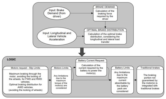
Figure 1.
Structure of the regenerative braking logic.
Regenerative motor torques are calculated based on brake demand in order to optimize energy recovery considering the optimal brake distribution if there are two motors and ensuring the stability of the vehicle by considering its slip limits. Then, it is also necessary to consider the limitations imposed by the maximum performance of the motors and batteries. Finally, traditional brakes can be integrated with the electric motor brake in order to ensure the deceleration intensity requested by the driver. All this while keeping the system close to optimal braking conditions.
The next subsections show the Equations and logics implemented in the Simulink® model for deploying a regenerative braking logic aimed at maximizing energy recovery.
2.1. Model Inputs and Outputs
The Simulink® model inputs are listed below.
- Brake demand (): value from 0 to 1, proportional to the force imposed by the driver on the brake pedal.
- Longitudinal vehicle deceleration (): positive value for vehicle deceleration.
- Lateral vehicle acceleration (): absolute value.
- Vehicle speed ( ): longitudinal vehicle speed.
- Angular velocity of the front wheels (): average value between left and right front wheels.
- Angular velocity of the rear wheels (): average value between left and right front wheels.
- Angular velocity of the front electric motor (): if the front motor is present.
- Angular velocity of the rear electric motor (): if the rear motor is present.
- Battery voltage ().
- Maximum charging current of the battery pack (): maximum current that the battery is able to accept in input from the motors at the moment considered.
The model outputs are listed below.
- Front brake pressure (): signal required for the control logic of the front braking system.
- Rear brake pressure (): signal required for the control logic of the rear braking system.
- Front motor torque (): output torque of the front electric motor.
- Rear motor torque (): output torque of the rear electric motor.
2.2. Brake Demand
The “BRAKE DEMAND” module receives the brake signal from the driver as an input and associates the required braking force to this signal.
The signal range is a value from 0 to 1, proportional to the master cylinder pressure and, hence, to the force imposed by the driver on the brake pedal, and the required braking force is imposed proportional to the maximum traditional brake force. Therefore, the value represents the maximum braking pressure, which is set a priori in the vehicle model.
The maximum force () that the traditional front brakes can generate at the tire contact patch is calculated in Equation (1):
is the maximum pressure that can be generated inside the master cylinder of the front brake system, is the total area of the brake pistons in the front calipers, is the dynamic coefficient of friction between the front brake pads and brake discs, is the average radius of application of the braking force on the front discs, and is the nominal rolling radius of the front wheels.
The maximum force () that the traditional rear brakes can generate at the tire contact patch is calculated in Equation (2):
is the maximum pressure that can be generated inside the master cylinder of the front brake system, is the total area of the brake pistons in the front calipers, is the dynamic coefficient of friction between the front brake pads and brake discs, is the average radius of application of the braking force on the front discs, and is the nominal rolling radius of the front wheels.
The maximum disc brake force () is the sum of the maximum front braking force () and the maximum rear braking force ().
The total braking force associated with the brake demand () is calculated in Equation (3).
2.3. Optimal Brake Distribution
The “OPTIMAL BRAKE DISTRIBUTION” module calculates the optimal brake distribution between the front and rear axle, taking the longitudinal () and lateral () vehicle acceleration as inputs. The braking distribution guarantees the correct stability of the vehicle during braking events.
The optimal braking distribution is calculated by taking into account the load transfer and the road friction coefficient to consider the road–tire adhesion limit that leads to locking the front and rear wheels at the same time.
The load on the front axle (), considering only the static weight and the longitudinal load transfer, is calculated in Equation (4):
is the vehicle mass, is the gravitational acceleration equal to 9.81 m/s2, is the wheelbase, is the center of gravity height, and is the longitudinal distance between the rear axle and the center of gravity of the vehicle, which is the difference between the wheelbase and the longitudinal distance between the front axle and the center of gravity (), as in Equation (5):
The load on the rear axle (), considering only the static weight and the longitudinal load transfer, is calculated in (6):
The load transfer, due to lateral acceleration, depends on the roll stiffness distribution and the roll angle.
The roll stiffness () of the front axle is calculated in Equation (7):
is the stiffness of the front suspension springs, is the stiffness of the front anti-roll bar, and is the front track of the vehicle.
The roll stiffness () of the rear axle is calculated in Equation (8):
is the stiffness of the rear suspension springs, is the stiffness of the rear anti-roll bar, and is the rear track of the vehicle.
The roll angle, , is calculated in Equation (9):
is the front sprung mass of the vehicle, is the rear sprung mass, is the height of the front roll center, and is the height of the rear roll center.
Finally, the front () and rear () load transfers, due to lateral acceleration, are calculated, respectively, in Equations (10) and (11):
Considering a single-wheel assembly, is half the front unsprung mass of the vehicle and is half the rear unsprung mass.
In the end, the reference loads on the front () and rear () axles, considering the inner wheel when cornering, is imposed, respectively, in Equations (12) and (13).
The model calculates the maximum forces on the front and rear axles considering the reference forces above.
The front total maximum braking force () is expressed in Equation (14), where is the road–tire friction coefficient.
The rear total maximum braking force () is expressed in Equation (15):
In the end, the optimal braking distribution () is defined as follows Equation (16):
2.4. Motors Request – Slip Limits
The Simulink® model includes three different logics for a front-wheel drive vehicle (FWD) with a single electric motor acting on the front axle, a rear-wheel drive vehicle (RWD) equipped with an electric motor acting on the rear axle, and for all-wheel drive vehicle (AWD) equipped with an electric motor for each axle.
2.4.1. FWD
For the FWD vehicle, the braking force required from the motor () is imposed as the minimum between the total braking force requested by the driver () and the front total maximum braking force (), multiplied by a safety coefficient ().
The front electric motor torque required () is calculated in Equation (17), taking into account the front wheel radius, the inertia of the wheels, the inertia of the differential, the inertia of the motor, and the transmission ratios.
is the time derivative; is the moment of inertia for a single front wheel; and are the moments of inertia of the transmission before and after the front motor reducer, respectively; is the moment of inertia of the front electric motor; is the gear ratio of the front differential; is the gear ratio of the front motor reducer; and is the general efficiency of the whole front transmission.
2.4.2. RWD
For the RWD vehicle, the braking force required from the motor () is imposed as the minimum between the total braking force requested by the driver () and the rear total maximum braking force (), multiplied by a safety coefficient ().
The rear electric motor torque required () is calculated in Equation (18), taking into account, as in the FWD case, the wheel radius, the inertia of the wheels, the inertia of the differential, the inertia of the motor, and the transmission ratios.
is the moment of inertia for a single rear wheel; and are the moments of inertia for the transmission before and after the front motor reducer, respectively; is the moment of inertia for the rear electric motor; is the gear ratio of the rear differential; is the gear ratio of the rear motor reducer; and is the general efficiency of the whole rear transmission.
2.4.3. AWD
For the AWD vehicle, the rear braking force associated with the driver demand () is calculated in Equation (19):
The front braking force associated with the driver demand () is instead the difference between and .
The braking force required from the front motor () is imposed as the minimum between the front total braking force requested by the driver () and the front total maximum braking force (), multiplied by a safety coefficient ().
Similarly, the braking force required from the rear motor () is imposed as the minimum between the rear total braking force requested by the driver () and the rear total maximum braking force (), multiplied by a safety coefficient ().
The Equations (17) and (18) are also used for the calculation of the required driving torques for the AWD case but they are calculated starting from the values of and , as explained in this section.
2.5. Motors Limits
In the subsystem called “Motors Limits” in Figure 1, the electric motor torques required—front () and rear ()—are compared with the maximum motor torques available at the motor RPM of the considered instant.
Outputs from this subsystem are the minimum value of torque, front () and rear (), between the maximum available and the required torque.
The maximum value of available torque for each motor (front and rear) is obtained by means of Simulink® lookup tables containing the torque curves of the motors as a function of the RPM of the motors themselves.
2.6. Battery Current Request
The “Battery Current Request” subsystem calculates the current that the motors should send to the battery if they provided the output braking torque from the “Motor Limits” subsystem.
The charging current of the front motor (), if present, is obtained with Relationship (20):
is the efficiency of the front motor at the point of operation considered, and it is obtained through the use of a two-dimensional Simulink® lookup table. This lookup table contains the front motor efficiency map; it receives the motor torque, , and the RPM of the motor in input and returns the efficiency at the operating point in output.
is the electric resistance of the front connection cables, and it is calculated as follows with Equation (21):
is the electric resistivity of copper (or in any case of the conductive material of the electric cables), is the total length of the connection cables of the front motor, and is the diameter of the front motor cables.
Similarly, the charging current of the rear motor (), if present, is obtained through Relationship (22):
is the efficiency of the rear motor at the point of operation considered, and it is obtained using a two-dimensional Simulink® lookup table that receives the motor torque and the RPM of the motor in input and returns the efficiency at the operating point in output.
is the electric resistance of the rear connection cables, and it is calculated as follows with Equation (23).
is the total length of the connection cables of the rear motor and is the diameter of the rear motor cables.
Finally, the total current that the motors should send to the battery () is provided by the sum of and .
2.7. Battery Limits
In the “Battery Limits” subsystem, the limits of the battery pack are considered; in particular, it is checked if the current that the motors should send to the battery does not exceed the maximum that can be absorbed by the battery pack at the moment ().
If this limit is not respected, it is necessary to limit the regenerative motor torques.
In case the motors do not need to be limited due to restrictions due to the battery pack, the following equations apply (Equations (24)–(26)):
is the charging current of the battery pack generated by the motor or motors, is the braking torque of the front motor, and is the braking torque of the rear motor.
In case of battery limitations, Euqations (24)–(26) are not valid. The current generated by the motor or motors is obtained through Equation (27) and the other two quantities are calculated as shown in the following sections, depending on the type of vehicle: FWD, RWD, or AWD.
2.7.1. FWD
For FWD vehicles, in the event of battery limitations, the regenerative front motor torque is recalculated from the maximum charging current, as in Equation (28):
is the actual efficiency of the front electric motor (in the case of an FWD vehicle), calculated with a Simulink® lookup table containing an efficiency map of the front motor.
2.7.2. RWD
Similar to the case of FWD vehicles, for RWD vehicles, in the event of battery limitations, the regenerative rear motor torque is recalculated based on the maximum absorbable current, as in Equation (29):
is the actual efficiency of the rear electric motor (in the case of an RWD vehicle), calculated with a Simulink® lookup table containing an efficiency map of the rear motor.
2.7.3. AWD
For AWD vehicles, the maximum power that can be sent to the battery by the motors is divided between the front () and rear () motors by means of the optimal braking distribution ratio, as in Equations (30) and (31):
By applying the optimal distribution to the power, the optimal distribution between the braking forces of the two axles is obtained, with an approximation due to losses related, in turn, to the resistance of the connection cables. In fact, the power is provided by the product between the force and the speed, and the longitudinal speed can be considered constant between the two axles; therefore, distributing the power in a certain way between the two axles means distributing the braking forces in the same way.
The maximum regenerative torque () that can be obtained from the front motor, exploiting the absorbable power, , of the battery pack, is provided by Relation (32).
is the electrical efficiency of the front motor at the operating point characterized by the parameters and , obtained thanks to Simulink® lookup tables containing efficiency maps of the front motor.
At this point of the model, a further check is carried out: it is verified that is not greater than , calculated as an output by the “Motors Limits” subsystem.
If is not greater than , the hypothetical front regenerative torque () is equal to ; vice versa, it is equal to .
Moreover, if is not greater than , the hypothetical charging power provided by the rear motor () is equal to ; otherwise, is calculated with Equation (33):
is the current that the front motor sends to the battery pack when it produces a regenerative motor torque equal to .
is calculated as follows in Relation (34):
is the electrical efficiency of the front motor at the operating point characterized by the parameters and , obtained thanks to a Simulink® lookup table containing an efficiency map of the front motor.
The hypothetical rear regenerative torque () is calculated using the Equation (35), starting from the power .
is the electrical efficiency of the rear motor at the operating point characterized by the parameters and , obtained thanks to Simulink® lookup tables containing efficiency maps of the rear motor.
Now, a further check is carried out: it is verified that is not greater than , calculated as output by subsystem “Motors Limits”.
If is not greater than , the actual rear regenerative torque () is equal to , and is equal to ; vice versa, is equal to , and in this case, it is necessary to recalculate the regenerative front motor torque as in Equation (36).
is the electrical efficiency of the front motor at the operating point characterized by the parameters and , obtained thanks to Simulink® lookup tables containing efficiency maps of the front motor.
is calculated in Equation (37):
is the current that the rear motor sends to the battery pack when it produces a regenerative motor torque equal to .
is calculated as follows in Equation (38):
is the electrical efficiency of the rear motor at the operating point characterized by the parameters and , obtained thanks to a Simulink® lookup table containing an efficiency map of the front motor.
2.8. Traditional Brakes
The “Traditional Brakes” subsystem calculates the pressure on the front () and rear () master cylinders of the brake system necessary to integrate the braking forces provided by the motor or motors in such a way as to guarantee the total braking force requested by the driver.
Moreover, the integration of braking through the traditional brake system ensures that the system comes as close as possible to the condition of optimal braking distribution to guarantee vehicle stability.
If only the motor (or motors) is able to guarantee the braking request from the driver, the pressures and are imposed equal to the null value; vice versa, the model must calculate the two pressure values.
In this second case, is calculated as in Equations (39) if the value resulting from (39) is smaller than ; otherwise, is imposed equal to , while is calculated as in Equations (40) if the value resulting from (40) is smaller than ; otherwise, is imposed equal to .
3. Results
This section reports the results of simulation tests carried out with VI-CarRealTime® on an FWD, an RWD, and an AWD car to check the braking efficiency and stability of a vehicle equipped with the logic presented in this paper.
Finally, through the Simulink® TEST model [1], the energy saving obtained through the regenerative braking logic is estimated.
3.1. Reference Vehicles
Three fully electric compact cars were taken as reference vehicles: one with front-wheel drive with an electric motor acting on the front axle, one with rear-wheel drive with an electric motor acting on the rear axle, and one with all-wheel drive with an electric motor for each axle.
The three vehicles share the characteristics shown in Table 1.

Table 1.
Reference vehicles characteristics.
Figure 2 represents the torque and power curves of the motor for both the FWD and RWD vehicles and for the two motors of the AWD vehicle.
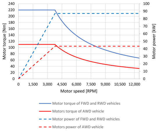
Figure 2.
Torque and power of electric motors of FWD, RWD, and AWD vehicles.
Table 2 shows the characteristics of the braking system of the three vehicles. If the vehicles are equipped with the regenerative braking logic, the front and rear master cylinders should be controlled by the logic independently; otherwise, there is a master cylinder controlled by the force input on the brake pedal, which distributes the pressure (total pressure equal to 15 MPa) between the front and rear cylinders with a bias on the front equal to 0.65.
Table 2.
Braking system characteristics.
Table 3 shows the main suspension characteristics of the three vehicle models, useful for defining the constant parameters of the regenerative logic. The three vehicles do not feature anti-roll bars for simplicity.
Table 3.
Suspension characteristics.
Table 4 shows the characteristics of the battery pack of the reference vehicles.
Table 4.
Battery pack characteristics.
The available capacity of the battery pack is the portion of capacity that can actually be used during vehicle operation. It differs from the nominal capacity, which is instead the real battery capacity, without considering that, during the operation of the vehicle, there will be limitations that will ensure that this capacity is not fully used in order to preserve the battery from premature decay.
When the three vehicles are equipped with the regenerative braking logic described in this article, a minimum speed equal to 15 km/h is defined for the activation of regenerative recovery, and the safety coefficients and are both set equal to 0.9; finally, the road–tire friction coefficient, , considered in the logic is set to constant.
Furthermore, none of the vehicles analyzed are equipped with an ABS system.
3.2. Test of the Regenerative Braking Logic
In this section, straight braking tests performed with VI-CarRealTime® are presented to show how the regenerative braking logic object of this paper acts on the regenerative motor torque and on the pressure in the traditional brake system.
The tests are carried out for the three vehicle types (FWD, RWD and AWD), equipped with RB logic with the coefficient constant equal to 1.
Table 5 shows the parameters of the tests; in particular, the initial vehicle speed is set equal to 108 km/h (30 m/s). At the start of the test (“start time” equal to zero seconds), 100% brake demand is achieved linearly in 10 s (“ramp up time”). The test ends when the vehicle stops. Therefore, a brake demand equal to 1 may not be reached during the test. The braking imposed was specifically chosen not to be very intensive so as not to lead to wheel locking or vehicle instability.
Table 5.
Parameters of straight braking test.
Figure 3 shows the speed of the three vehicles (FWD, RWD, and AWD) featuring the RB logic, as well as the brake demand during the straight braking test. Figure 3 also shows the motor torque and the brake pressure during the tests. Only the brake pressures on the left side of the vehicle are graphically represented because the left and right pressures are the same.
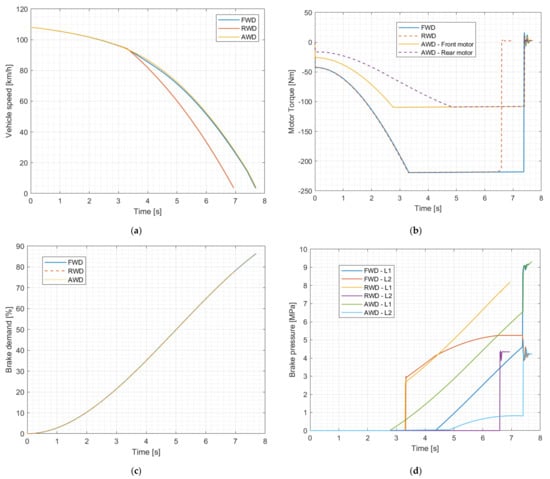
Figure 3.
Straight braking tests. (a) Vehicle speed; (b) motor torque; (c) brake demand; (d) brake pressure at the front left wheel (L1) and at the rear left wheel (L2).
Figure 3 shows that, in the initial stage of braking, only the braking torque of the motor (or motors) intervenes, while when braking becomes more intensive, the contribution of the traditional brakes integrates the regenerative braking.
3.3. Braking Performance and Handling
In this section, tests performed with the VI-CarRealTime® software are presented to check the performance and handling of vehicles equipped with RB logic.
3.3.1. Straightline Panic Brake
First of all, a panic braking test on a straightline is carried out via VI-CarRealTime® to verify the braking effectiveness of the vehicle equipped with RB logic. The behavior of the latter is compared with that of the same vehicle without regenerative braking.
The tests are carried out for the three vehicle types, as stated before (FWD, RWD, and AWD), and with two different coefficients of road surface friction (1 for dry tarmac; 0.7 for a wet surface), remembering that the model coefficient in the RB logic is defined as a constant value because it is not possible to know the real road friction coefficient on board the vehicle.
In the RB logic, the model coefficient is normally set equal to 1. The tests with a road friction coefficient of 0.7 for vehicles equipped with regenerative braking logic, are also repeated with a model coefficient set to 0.7 to verify the influence of the correct definition of this parameter for panic braking performance.
These tests are used to verify that the RB logic performs well in comparison with a standard vehicle (i.e., without any regenerative braking), even in the case of a low friction coefficient. For this reason, no tests were carried out below the value of 0.7: as a matter of fact, any standard vehicle without an anti-lock braking system (ABS) performs poorly in a panic stop maneuver on wet pavement because wheel locking occurs immediately; therefore, it makes no sense to take its behavior as a reference. The same goes for the tests of the next subsection. Braking in turn maneuvers can be carried out successfully only if an appropriate ABS logic is implemented on the vehicle, either with or without a regenerative braking logic. An appropriate ABS strategy, downstream of the RB logic, also considering the contribution of the electric motors during braking, is therefore required. An example of ABS logic suitable for the purpose, as already anticipated, is presented in [9].
Table 6 shows the test parameters: the initial vehicle speed is set to 90 km/h; this speed is maintained for 1 s (“start time”), then 100% brake demand is achieved linearly in 1 s (“ramp up time”).
Table 6.
Parameters of straight panic braking test.
Figure 4 shows the results of various panic brake tests carried out on a straightline.
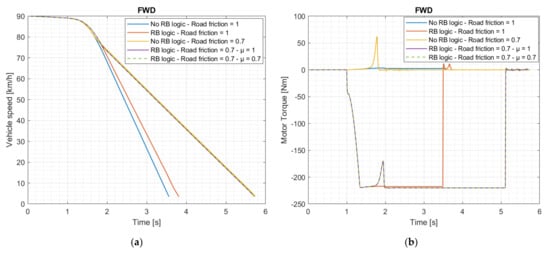
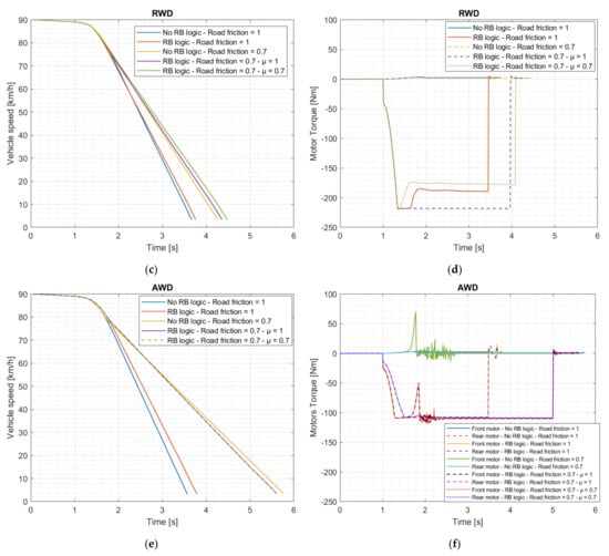
Figure 4.
Vehicle speeds and motor torques during the straightline panic brake tests. In particular: (a) vehicle speed in tests with FWD vehicles (with and without RB logic) on surfaces with road friction coefficients equal to 1 and 0.7; (b) motor torque in tests with FWD vehicles (with and without RB logic) on surfaces with road friction coefficients equal to 1 and 0.7; (c) vehicle speed in tests with RWD vehicles (with and without RB logic) on surfaces with road friction coefficients equal to 1 and 0.7; (d) motor torque in tests with RWD vehicles (with and without RB logic) on surfaces with road frictions coefficient equal to 1 and 0.7; (e) vehicle speed in tests with AWD vehicles (with and without RB logic) on surfaces with road friction coefficients equal to 1 and 0.7; (f) motor torque in tests with AWD vehicles (with and without RB logic) on surfaces with road friction coefficients equal to 1 and 0.7.
As shown by Figure 4a,c,e, the RB logic leads to a slight deterioration of the panic braking performance of all three vehicles (FWD, RWD, and AWD) on road surfaces with a friction coefficient equal to 1. As for surface tests with a model coefficient of friction equal to 0.7, the FWD vehicles equipped with RB logic behave like the vehicle without the regenerative braking; the RWD vehicles equipped with RB logic have slightly lower performance in the panic brake test compared with the RWD vehicle without regenerative braking; and, finally, the RB logic in AWD vehicles leads to an improvement in panic braking compared to the same vehicle not equipped with RB logic.
In these tests, the contribution of the variation of the model coefficient assumed that the RB logic does not lead to substantial variations in the behavior of the cars.
It can be said that effective panic braking has been achieved through RB logic even without an ABS system.
Furthermore, unlike what happens on vehicles equipped with classic regenerative braking logics in the literature, the RB logic object of this paper also allows for an intensive intervention of electric motors in generator mode for panic braking, as can be seen from panels (b), (d), and (f) in Figure 4.
Figure 5 shows the mean between the angular speeds of the left and right front wheels and the mean between the angular speeds of the left and right rear wheels for all the FWD vehicles in the panic brake tests (with road friction coefficients equal to 1 and 0.7): the vehicle without RB logic, the vehicle with RB logic with a model coefficient equal to 1, and the vehicle with RB logic with a model coefficient equal to 0.7.
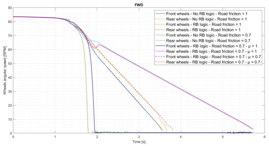
Figure 5.
Mean between the angular speeds of the left and right wheels (front mean and rear mean) of the FWD vehicles (with and without RB logic) during the straight panic brake tests on road surfaces with friction coefficients equal to 1 and 0.7.
As shown by the graph in Figure 5, in the tests with a road friction coefficient equal to 0.7, all the vehicles lock the front wheels and not the rear wheels, even those equipped with RB logic; this is positive to ensure stability, as it is necessary to avoid locking the rear wheels or, in any case, to assure the front wheels lock before the rear ones.
Figure 6 shows the mean between the angular speeds of the left and right front wheels and the mean between the angular speeds of the left and right rear wheels for all the RWD vehicles in the panic brake tests.
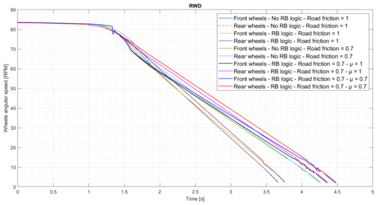
Figure 6.
Mean between the angular speed of the left and right wheels (front mean and rear mean) of the RWD vehicles (with and without RB logic) during the straight panic brake tests on road surfaces with friction coefficients equal to 1 and 0.7.
As shown in Figure 6, in all the tests (with road friction coefficients equal to 1 and 0.7), all the vehicles lock the front and rear wheels almost simultaneously. The tests with RWD vehicles, therefore, achieved excellent results.
Finally, Figure 7 shows the mean between the angular speeds of the left and right front wheels and the mean between the angular speeds of the left and right rear wheels for all the AWD vehicles in the panic brake tests.
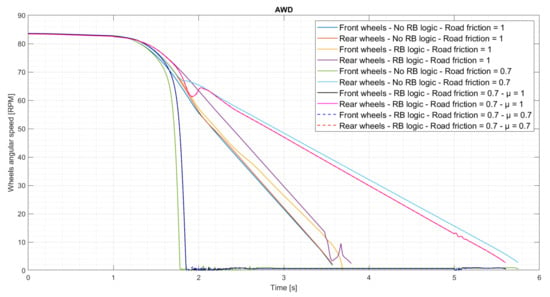
Figure 7.
Mean between the angular speeds of the left and right wheels (front mean and rear mean) of the AWD vehicles (with and without RB logic) during the straight panic brake tests on road surfaces with friction coefficients equal to 1 and 0.7.
3.3.2. Braking in Turn
The “braking in turn” test consists of driving along a constant radius curve at a predetermined speed and then braking with a target deceleration. Table 7 shows the related parameters.
Table 7.
Parameters of the “braking in turn” test.
In this test, the vehicle, traveling at 126 km/h, turns into a circular trajectory with a radius of 300 m. After 5 s, the braking phase begins with target deceleration equal to 10 m/s2. The simulation ends when the vehicle reaches zero speed.
Figure 8 shows the vehicle speeds and motor torques of FWD, RWD, and AWD vehicles for all the “braking in turn” tests performed.
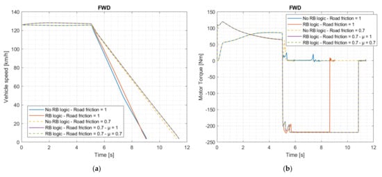
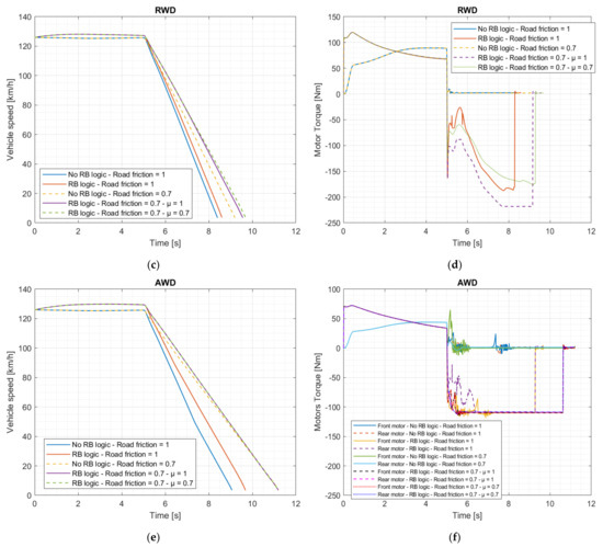
Figure 8.
Vehicle speeds and motor torques during the “braking in turn” tests. (a) Vehicle speed of FWD vehicles (with and without RB logic) on surfaces with road friction coefficients equal to 1 and 0.7; (b) motor torque of FWD vehicles (with and without RB logic) on surfaces with road friction coefficients equal to 1 and 0.7; (c) vehicle speed of RWD vehicles (with and without RB logic) on surfaces with road friction coefficients equal to 1 and 0.7; (d) motor torque of RWD vehicles (with and without RB logic) on surfaces with road friction coefficients equal to 1 and 0.7; (e) vehicle speed of AWD vehicles (with and without RB logic) on surfaces with road friction coefficients equal to 1 and 0.7; (f) motor torques of AWD vehicles (with and without RB logic) on surfaces with road friction coefficients equal to 1 and 0.7.
As shown by Figure 8, panels (a), (c), and (e), the RB logic leads to a slight deterioration of the braking performance in the “braking in turn” test for the FWD vehicle on the surface with a coefficient of friction equal to 0.7, for the RWD vehicle on both surfaces, and for the AWD vehicle on the surface with a friction coefficient equal to 1. In the remaining cases, the RB logic does not lead to substantial differences in the behavior of the vehicle when braking in cornering compared to the case of a vehicle without regenerative braking.
Even in these tests, the contribution of the variation of the RB logic model coefficient does not lead to substantial variations in the behavior of the cars.
The RB logic object of this paper allows for an intensive intervention of the electric motors in generator mode, as can be seen from panels (b), (d), and (f) of Figure 8.
Figure 9 shows the trajectory of the center of gravity of the vehicles during the tests. In particular, the coordinates of the center of gravity of the vehicle are reported along two orthogonal axes, where the initial position of the vehicle at the start of the test corresponds to zero coordinates at the origin of the orthogonal coordinate system.
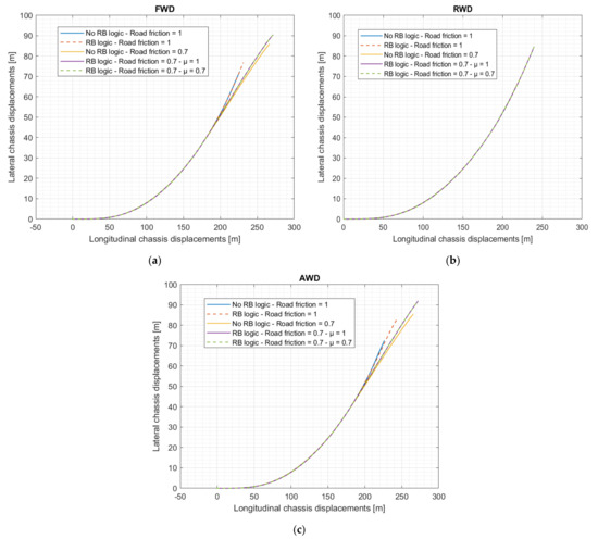
Figure 9.
Lateral chassis displacements as a function of longitudinal chassis displacements during “braking in turn” tests. In particular: (a) tests with the FWD vehicle; (b) tests with the RWD vehicle; (c) tests with the AWD vehicle.
Figure 10 shows the angular speed of each wheel for all the FWD vehicles in the “braking in turn” tests (with road friction coefficients equal to 1 and 0.7): the vehicle without RB logic, the vehicle with RB logic with a model coefficient equal to 1, and the vehicle with RB logic with a model coefficient equal to 0.7.
Figure 10.
Angular speed of each wheel of the FWD vehicles (with and without RB logic) during “braking in turn” tests, where L1 is the front left (outer) wheel, R1 the front right (inner) wheel, L2 the rear left (outer) wheel, and R2 the rear right (inner) wheel. In particular: (a) tests on a road surface with a friction coefficient equal to 1; (b) tests on a road surface with a friction coefficient equal to 0.7.
As can be seen from the graphs in Figure 10, in the tests with a road friction coefficient equal to 1, the vehicle without RB logic first locks the front inner (right) wheel; then the rear inner (right) wheel; and then, finally, the front outer (left) wheel. The rear outer (left) wheel is not locked during the test. The vehicle equipped with RB logic, on the other hand, locks only the front wheels (the front inner wheel first and the front outer only toward the end of the test). For this test, the regenerative braking logic can, therefore, lead to benefits in terms of vehicle stability.
In the tests with a road friction coefficient equal to 0.7, the vehicle without RB logic locks the front wheels and not the rear wheels, while the vehicle equipped with RB logic has the same behavior with model parameters equal to both 1 and 0.7, and it locks the front wheels first and the then the rear inner (right) wheel. On the low road surface friction, the RB logic, therefore, resulted in locking the rear wheel inside the curve as a detrimental effect, and it delayed the locking of the front outer (left) wheel with respect to the front inner (right) one as compared to the case of the vehicle without regenerative braking.
Figure 11 shows the angular speed of each wheel for all the RWD vehicles in the “braking in turn” tests.

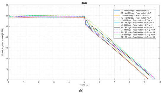
Figure 11.
Angular speed of each wheel of the RWD vehicles (with and without RB logic) during the “braking in turn” tests, where L1 is the front left (outer) wheel, R1 the front right (inner) wheel, L2 the rear left (outer) wheel, and R2 the rear right (inner) wheel. In particular: (a) tests on a road surface with a friction coefficient equal to 1; (b) tests on a road surface with a friction coefficient equal to 0.7.
As can be seen from the graphs in Figure 11, in the RWD tests, there is never a complete locking of any wheel, for any vehicle.
Finally, Figure 12 shows the angular speed of each wheel for all the AWD vehicles in the “braking in turn” tests.
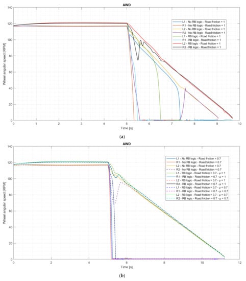
Figure 12.
Angular speed of each wheel of the AWD vehicles (with and without RB logic) during the “braking in turn” tests, where L1 is the front left (outer) wheel, R1 the front right (inner) wheel, L2 the rear left (outer) wheel, and R2 the rear right (inner) wheel. In particular: (a) tests on a road surface with a friction coefficient equal to 1; (b) tests on a road surface with a friction coefficient equal to 0.7.
As can be seen from Figure 12, in the tests with a road friction coefficient equal to 1, the vehicle without RB logic first locks the front inner (right) wheel; then the rear inner (right) wheel; and then, finally, the front outer (left) wheel. The rear outer (left) wheel is not locked during the test. The vehicle equipped with RB logic, on the other hand, locks only the front wheels (the front inner wheel first and the front outer wheel afterward). For this test, the regenerative braking logic, therefore, led to benefits in terms of AWD vehicle stability, as with the front-wheel drive vehicle.
In the tests with a road friction coefficient equal to 0.7, the vehicle without RB logic locks the front wheels and not the rear wheels, as does the vehicle equipped with RB logic, which has the same behavior with model parameters equal to both 1 and 0.7.
Therefore, on the low road friction surface, the RB logic for this vehicle does not lead to substantial changes in the behavior of the vehicle itself.
3.4. Energy Consumption and Recovery Estimation
This section uses the test model described in paper [19] to estimate the energy savings associated with the adoption of the regenerative braking logic (RB logic) covered by this paper in the three vehicles (FWD, RWD, and AWD). In particular, the RB logic is integrated into the TEST model [19], and through the graphic user interface of the model, it is possible to activate this logic or keep it deactivated and simulate the braking phase as described in paper [19], which is considered a classic, traditional, or standard regenerative braking logic, the simplest adopted on the market.
The energy consumption of the three vehicles (FWD, RWD, and AWD) equipped with RB logic, without brake recovery, and equipped with a classic and simple regenerative braking logic—commonly adopted on electric vehicles on the market, which will be explained later—has been estimated on the basis of two different standard driving cycles (WLTC and US06), keeping in mind that energy consumption is strongly influenced by the driving cycle considered [22]. Vehicles without regenerative recovery and vehicles equipped with classic logic are used to estimate the energy savings guaranteed by the RB logic.
3.4.1. Vehicle Models
The vehicles subject to simulations using the TEST model [19] are the same (FWD, RWD, and AWD) as those previously analyzed through the tests with VI-CarRealTime, i.e., those described in Section “3.1 Reference Vehicles” with characteristics shown in Table 1, Table 2, Table 3 and Table 4. The AWD vehicle features a 50% distribution of the drive torque between front and rear in acceleration and, in the case of regenerative recovery with classic logic, in braking as well.
As already mentioned, three simulations are carried out for each vehicle type, one with RB logic, one without braking energy recovery, and one with a classic regenerative braking logic according to [19].
In the case of classic regenerative braking, maximum torque is considered for regenerative braking, which has a trend that increases linearly as a function of the time elapsed from the beginning of braking and then reaches a predefined maximum value (absolute value only). This is the approach typically adopted in electric vehicles on the market. This approach is also the one adopted in the waste collection vehicle in the prototype state used for the validation of the TEST model in paper [19]. The values of the maximum regenerative braking trend (Figure 13), i.e., the slope (22.5 Nm/s) of the increasing linear section and the constant plateau value (50 Nm), are also taken from the waste collection vehicle considered in paper [19]. These values are used for the simulations of the FWD and RWD vehicles, while for the AWD vehicle, such values are equally split between the two motor units (11.25 Nm/s and 25 Nm) so that the total contribution of the maximum regenerative braking is the same as the other vehicles.
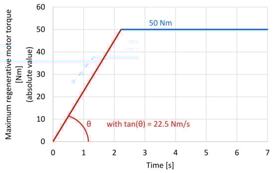
Figure 13.
Maximum regenerative motor torque trend for the classic regenerative braking logic for the FWD and RWD vehicles.
For both regenerative braking logics, a minimum speed of 15 km/h is set for the activation of the logic itself. Below this speed, there is no energy recovery during braking.
The simulations were carried out starting with a battery SOC equal to 70% so as to exploit the central range of SOC in such a way that only limitations due to the maximum current and maximum power (in absolute value, positive and negative, in input and output from the battery pack) come into play within this range, therefore avoiding the more stringent limitations related to the extremes of the SOC range.
3.4.2. WLTP Procedure
First, consumption and energy recovery are estimated on the regulated cycle known as WLTC (Worldwide Harmonized Light-Duty Vehicles Test Cycle), as described in the WLTP procedure (Worldwide Harmonized Light-Duty Vehicles Test Procedure) [23].
The standard in [23] differentiates various classes for the WLTC depending on the power/weight ratio. The vehicles examined have a maximum power of 87 kW and a weight of 1548.4 kg with a power/weight ratio of approximately 56.2 W/kg; therefore, they fall within class 3. Furthermore, the maximum speed of these vehicles is higher than 120 km/h; therefore, they fall into subclass 3b. The class 3b WLTC is composed of the phases “Low3”, “Medium3-2”, “High3-2”, and “Extra High3”, as defined by [23].
The tests with the TEST model [19] were then carried out on the class 3b WLTC cycle, which has a duration of 1800 s on a distance of about 23.3 km.
Figure 14 reports some results of the simulations carried out for the FWD vehicles.
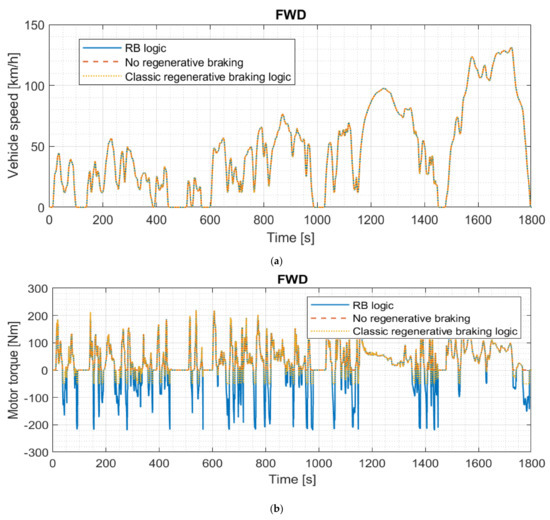
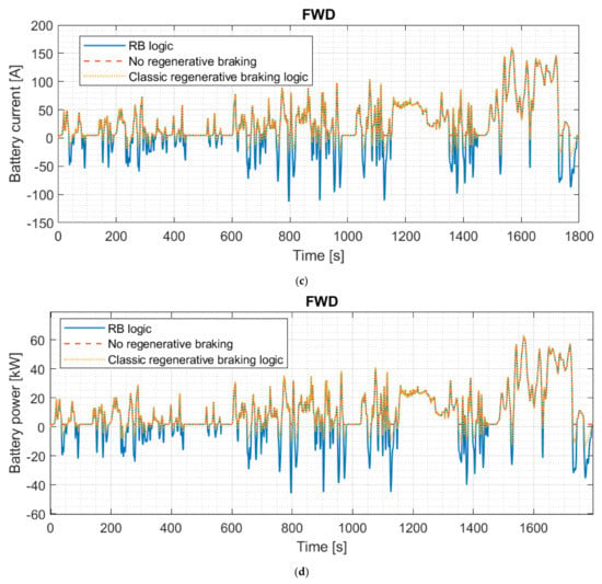
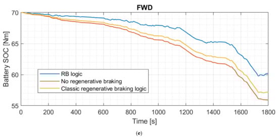
Figure 14.
Results of FWD vehicle simulations on the class 3b WLTC. (a) Vehicle speed; (b) motor torque; (c) battery current; (d) output (positive) and input (negative) power to the battery pack; (e) battery SOC.
In Figure 14b–d, it can be seen how the regenerative braking of the RB logic is decidedly more intensive than that of the vehicle equipped with classic logic. This results in a higher SOC at the end of the driving cycle, as can be seen in Figure 14e.
FWD vehicles, as well as RWD and AWD vehicles, manage to faithfully follow the class 3b WLTC. Graph (a) of Figure 14 is, therefore, basically the same for all vehicle types.
Figure 15 reports some results of the simulations carried out for the RWD vehicles.

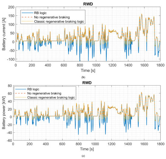
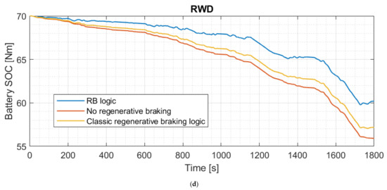
Figure 15.
Results of the RWD vehicle simulations on the class 3b WLTC. (a) Motor torque; (b) battery current; (c) output (positive) and input (negative) power to the battery pack; (d) battery SOC.
Figure 15a–c show how the regenerative braking of the RB logic is decidedly more efficient for the RWD vehicle as well. This again improves the average SOC during the driving cycle, as shown in Figure 15d.
Figure 16 reports some results of the simulations carried out for the AWD vehicles.
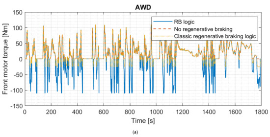
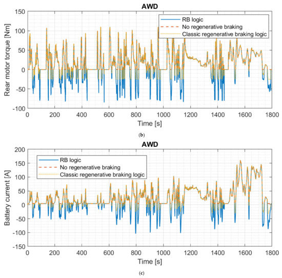
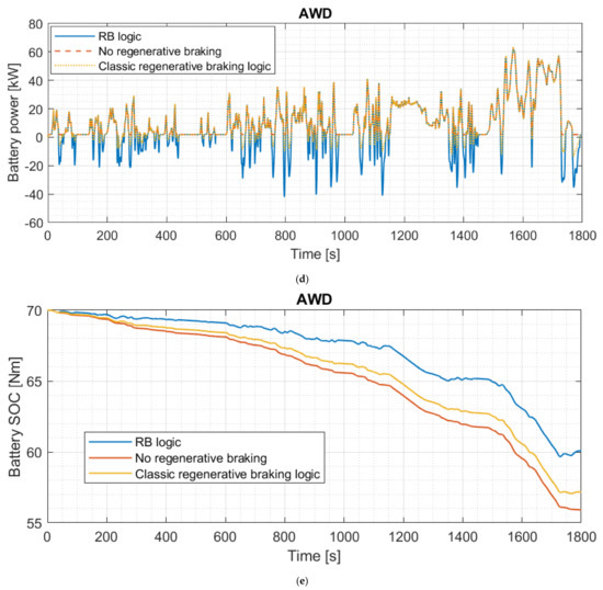
Figure 16.
Results of simulations with AWD vehicles on the class 3b WLTC. In particular: (a) front motor torque; (b) rear motor torque; (c) battery current; (d) output (positive) and input (negative) power to the battery pack; (e) battery SOC.
The same considerations made for FWD and RWD vehicles can also be made for the simulations of AWD vehicles, i.e., those from Figure 16a d; it can be seen how the regenerative braking of the RB logic is an improvement over the traditional logic. This results in a lower decrease in SOC during the driving cycle, as can be seen in Figure 16d.
Table 8 reports energy consumption and SOC on the class 3b WLTP cycle, for the FWD, RWD, and AWD vehicles, equipped with RB logic, classic regenerative braking logic, and without braking recovery. The final SOC of the simulation on the single cycle is also reported, remembering that the initial SOC was set to equal 70%. The specific energy consumption is also reported on the basis of the distance traveled by the vehicles during the simulation.
Table 8.
Consumption in the class 3b WLTC.
3.4.3. US06 Cycle
Consumption and energy recovery are also estimated on the SFTP-US06-regulated cycle, described in the EPA Supplemental Federal Test Procedure (SFTP).
We also chose to carry out simulations on the US06 cycle to obtain results on a cycle with more intense acceleration and deceleration levels than the relatively mild ones of the WLTP.
The simulations were performed again by means of the TEST model [19].
The US06 cycle has a duration of 600 s, and the vehicle travels about 12.9 km on this cycle.
Figure 17, Figure 18 and Figure 19 graphically report some results of the simulations carried out for the FWD, RWD, and AWD vehicles on the US06 cycle.
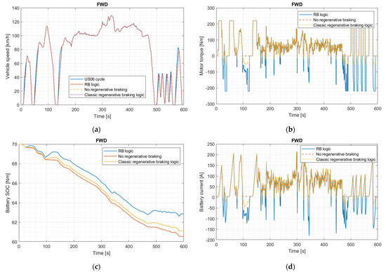
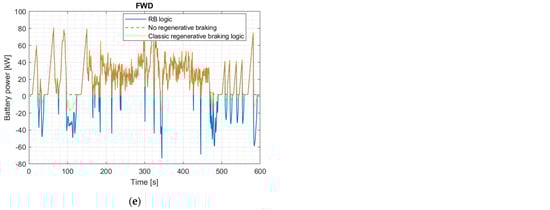
Figure 17.
Results of simulations with FWD vehicles on the US06 cycle. In particular: (a) vehicle speed; (b) motor torque; (c) battery SOC; (d) battery current; (e) output (positive) and input (negative) power to the battery pack.
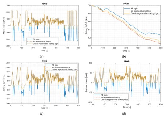
Figure 18.
Results of simulations with RWD vehicles on the US06 cycle. In particular: (a) motor torque; (b) output (positive) and input (negative) power to the battery pack; (c) battery current; (d) battery SOC.
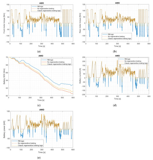
Figure 19.
Results of simulations with AWD vehicles on the US06 cycle. In particular: (a) front motor torque; (b) rear motor torque; (c) battery SOC; (d) battery current; (e) output (positive) and input (negative) power to the battery pack.
As shown in section (a) of Figure 17, the FWD vehicle (both with the two regenerative braking logics and without any) is unable to follow the target profile defined by cycle US06; the vehicle speed deviates from the target in some acceleration phases. The same situation was found for all RWD and AWD vehicles, whose speed profiles are the same as the FWD vehicle, i.e., section (a) of Figure 17. As a matter of fact, the vehicles in question lack the torque and performance to faithfully follow the US06 standard cycle, which is particularly demanding with regard to acceleration phases.
Again, on the US06 cycle, braking energy recovery is generally higher for vehicles equipped with the RB logic presented in this paper, and this is true for all vehicles considered (FWD, RWD, and AWD). This can be easily seen in Figure 17b–e; Figure 18a,c,d; and Figure 19a,b,d,e.
Table 9 reports the energy consumption and SOC on the US06 cycle, again for all three vehicles featuring RB logic, traditional braking logic, and without braking recovery. The final SOC of the simulation on the single cycle is also reported, remembering that the initial SOC was set to equal 70%. The specific energy consumption is also reported.
Table 9.
Consumption on the US06 cycle.
4. Discussion
In this paper, a regenerative braking logic aimed at the optimization of energy recovery during braking is presented to be adopted on electric vehicles with FWD, RWD, or AWD (equipped with a motor for each axle) transmission layouts.
Section 3.2 shows the operation of the RB logic and, in particular, how regenerative torque and pressures in the front and rear brake systems intervene during the braking phase in a normal braking maneuver.
In Section 3.3, a panic braking maneuver is used to verify that the RB logic does not lead to a loss of vehicle stability. A comparison is made with similar vehicles without any regenerative braking logic. Section 3.3.1 presents straightline panic braking and shows how deceleration performance is not made worse when compared to a reference vehicle without regenerative recovery. Section 3.3.2, on the other hand, shows the correct operation of the RB logic even during a phase of intense braking when cornering.
Section 3.4 demonstrates the energy savings that can be obtained thanks to the use of the RB logic, either on the WLTC or on the more demanding US06 cycle. For both cycles and for all vehicle types (FWD, RWD, and AWD), a comparison is also made with the consumption obtained by implementing a standard type of regenerative logic.
The RB logic in the FWD vehicle made it possible to save 7.70 kWh (savings of 30.3%) of battery on the class 3b WLTC and 7.66 kWh (savings of 24.4%) on the US06 cycle compared to the same vehicle without regenerative recovery. Comparing the RB logic with a classic logic commonly adopted on the market, a saving of 5.43 kWh (savings of 23.4%) on the WLTC and 5.75 kWh (savings of 19.5%) on the US06 cycle was found instead.
The RB logic in the RWD vehicle made it possible to save 7.71 kWh (savings of 30.3%) of battery on the class 3b WLTC and 7.65 kWh (savings of 24.4%) on the US06 cycle compared to the same vehicle without regenerative recovery. Comparing the RB logic with a classic logic commonly adopted on the market, a saving of 5.45 kWh (savings of 23.5%) on the WLTC cycle and 5.75 kWh (savings of 19.5%) on the US06 cycle was found instead.
Finally, the RB logic in the AWD vehicle made it possible to save 7.52 kWh (savings of 29.5%) of battery on the class 3b WLTC and 7.50 kWh (savings of 23.9%) on the US06 cycle compared to the same vehicle without regenerative recovery. Comparing the RB logic with a classic logic commonly adopted on the market, a saving of 5.25 kWh (savings of 22.6%) on the WLTC cycle and 5.59 kWh (savings of 19.0%) on the US06 cycle was found instead.
The RB logic performs better in terms of energy savings on the relatively mild WLTC compared to the US06.
The different tests reported in this paper were all carried out with a constant tire-road friction model coefficient (); in particular, in the base case, is equal to 1.
By setting to be constant in the model, however, it is possible to optimize the operation of the RB logic for a certain friction coefficient and then act on the two safety limits ( and ) to avoid locking the drive wheels in other cases (with different coefficients of adhesion) due to regenerative braking alone, even before the braking system has intervened.
For the correct operation of the RB logic, it is necessary to correctly set all the vehicle parameters within the model and, if necessary, to use the unknown parameters as calibration values. It is also necessary to tune the braking system of the vehicle correctly for a correct distribution between the maximum pressures in the front and rear braking system in particular in order to guarantee correct braking even in the event of 100% brake demand.
Another interesting opportunity is the adoption of an ABS strategy specifically tuned for the RB logic, where control of the regenerative torques offered by the electric motors is also taken into account when necessary. In this way, it is possible to optimize the logic for a given condition, for example, in different road friction conditions.
The RB logic also lends itself to further optimization in cases where a real-time estimate of the road friction coefficient is available. Review paper [24] reports various techniques for this purpose, as well as the role and practicality of this coefficient in the vehicle system.
Paper [25] reports another review on the topic. Various estimation methods are also classified based on:
- Offboard sensors (laser profilometer, camera, intelligent tire with accelerometer, ultrasonic transmitter, receiver, etc.);
- Onboard sensors and vehicle dynamics model (lateral, longitudinal, and coupled dynamics model);
- Data-driven (neural networks and so on).
The RB logic model has a modular structure, so it lends itself to modifications and improvements. Here are some aspects concerning possible future developments of the RB logic:
- Integration of the logic with a model for the estimation of the tire–road friction coefficient, as stated above;
- Improvement of the tire simulation model—in particular, the tire–road interaction, for example, by implementing a fully nonlinear Pacejka Magic Equation;
- Integration of a specific ABS strategy also acting on the braking torques of the electric motors; see [9] for an example.
5. Conclusions
This paper presents a regenerative braking logic aimed at maximizing energy recovery when braking without compromising the stability of the vehicle. Such RB logic was tested on the vehicle dynamics models of FWD, RWD, and AWD compact cars.
In summary, the RB model ensures that the regenerative torque of the electric motor(s) is exploited to the maximum while also preventing the locking of drive wheels at the same time, and subsequently, if necessary, integrating motor braking with the action of the traditional brake system.
For FWD and RWD vehicles, the integration between regenerative and traditional braking also aids the optimal braking distribution and the maximization of regenerative braking at the same time.
In the case of an AWD vehicle, the logic aims to pursue, instant by instant, the optimal motor braking distribution on the basis of the longitudinal acceleration and related load transfer effects.
For the FWD and RWD compact cars, the RB logic makes it possible to save around 30% in terms of energy consumption on the class 3b WLTP cycle compared to a vehicle without regenerative recovery and about 23.5% compared to a vehicle equipped with a classic regenerative braking logic, commonly adopted on vehicles on the market according to [19]. On the US06 cycle, on the other hand, it made it possible to save 24.4% and 19.5%, respectively. Similar, promising results have been achieved with the AWD car.
Author Contributions
Conceptualization, G.S., D.C. and M.G.; methodology, G.S.; software, G.S.; validation, G.S. and D.C.; data curation, G.S.; writing—original draft preparation, G.S.; writing—review and editing, G.S., D.C. and M.G.; visualization, M.G. and D.C.; supervision, M.G. and D.C. All authors have read and agreed to the published version of the manuscript.
Funding
This research received no external funding.
Institutional Review Board Statement
Not applicable.
Informed Consent Statement
Not applicable.
Data Availability Statement
The data presented in this study are available on request from the corresponding author. The data are not publicly available due to University of Brescia privacy policy.
Conflicts of Interest
The authors declare no conflict of interest.
Appendix A
Table A1.
Nomenclature.
Table A1.
Nomenclature.
| Abbreviation | Description |
|---|---|
| ABS | From the German: Antiblockiersystem. Anti-lock system. Avoid locking the vehicle’s wheels when braking. |
| Lateral vehicle acceleration (of the center of gravity), absolute value 3 | |
| Total area of the brake pistons, front calipers 1 | |
| Total area of the brake pistons, rear calipers 1 | |
| APU | Auxiliary power unit |
| AWD | All-wheel drive vehicle |
| Optimal braking distribution 4 | |
| Brake demand (from 0 to 1) 3 | |
| CG | Center of gravity |
| Maximum charging current of the battery pack 3 | |
| Charging current of the battery pack generated by the motor or motors 4 | |
| Current that the front motor sends to the battery pack when it produces a regenerative motor torque equal to Tref F 4 | |
| Current that the rear motor sends to the battery pack when it produces a regenerative motor torque equal to Tref F 4 | |
| Total charging current generated by the motor or motors | |
| Charging current generated by the front motor 4 | |
| Charging current generated by the rear motor 4 | |
| EPA | Environmental Protection Agency |
| Total braking force request 4 | |
| Front braking force associated with the driver demand 4 | |
| Rear braking force associated with the driver demand 4 | |
| FLC | Fuzzy logic controllers |
| Theoretical total maximum braking force that the front axle can unload on the ground 4 | |
| Theoretical total maximum braking force that the rear axle can unload on the ground 4 | |
| Maximum braking force that the traditional brakes can unload on the ground 4 | |
| Maximum braking force that the traditional front brakes can unload on the ground 4 | |
| Maximum braking force that the traditional rear brakes can unload on the ground 4 | |
| Braking force required from the front motor 4 | |
| Braking force required from the rear motor 4 | |
| FWD | Front-wheel drive vehicle |
| Acceleration of gravity 1 | |
| Height of the front roll center 1 | |
| Height of the rear roll center 1 | |
| Height of the center of gravity of the vehicle 1 | |
| Longitudinal vehicle deceleration (positive value) 3 | |
| Moment of inertia of the transmission after the front motor reducer 1 | |
| Moment of inertia of the transmission after the rear motor reducer 1 | |
| Moment of inertia of the front electric motor 1 | |
| Moment of inertia of the rear electric motor 1 | |
| Moment of inertia of the transmission before the front motor reducer 1 | |
| Moment of inertia of the transmission before the rear motor reducer 1 | |
| Moment of inertia of a single front wheel 1 | |
| Moment of inertia of a single rear wheel 1 | |
| Stiffness of the front anti-roll bar 1 | |
| Stiffness of the rear anti-roll bar 1 | |
| The roll stiffness of the front axle 1 | |
| The roll stiffness of the rear axle 1 | |
| Stiffness of the front suspension springs 1 | |
| Stiffness of the rear suspension springs 1 | |
| Wheelbase 1 | |
| Distance between the front axle and the center of gravity of the vehicle 1 | |
| Distance between the rear axle and the center of gravity of the vehicle 1 | |
| Total length of the connection cables of the front motor 1 | |
| Total length of the connection cables of the rear motor 1 | |
| Vehicle mass 1 | |
| Half the front unsprung mass of the vehicle 1 | |
| Half the rear unsprung mass of the vehicle 1 | |
| Front sprung mass of the vehicle 1 | |
| Rear sprung mass of the vehicle 1 | |
| MRC | Model reference controllers |
| NNC | Neutral networks controllers |
| Hypothetical power absorbed by the battery pack, coming from the front motor, in the case of an AWD vehicle, with battery limitations 4 | |
| Hypothetical charging power provided by the rear motor 4 | |
| Charging power provided by the front motor in case of approximation error in the calculation of TmotR, for AWD vehicles 4 | |
| Hypothetical power absorbed by the battery pack, coming from the rear motor, in the case of an AWD vehicle, with battery limitations 4 | |
| PIDC | Proportional-integral-differential controllers |
| Front master cylinder brake pressure 4 | |
| Rear master cylinder brake pressure 4 | |
| Maximum pressure that can be generated inside the master cylinder of the front brake system 1 | |
| Maximum pressure that can be generated inside the master cylinder of the rear brake system 1 | |
| RB | Regenerative Braking |
| Electric resistance of the front connection cables 2 | |
| Electric resistance of the rear connection cables 2 | |
| Average radius of application of the braking force on the front discs 1 | |
| Average radius of application of the braking force on the rear discs 1 | |
| RPM | Revolutions per minute |
| RWD | Rear-wheel drive vehicle |
| Nominal rolling radius of the front wheels 1 | |
| Nominal rolling radius of the rear wheels 1 | |
| Safety coefficient for the braking force guarantee by the front motor, for avoiding the locking of the front driving wheels 1 | |
| Safety coefficient for the braking force guarantee by the rear motor, for avoiding the locking of the rear driving wheels 1 | |
| SFTP | Supplemental Federal Test Procedure |
| SMC | Sliding-mode controllers |
| SOC | Battery State of Charge |
| Hypothetical front regenerative torque, minimum value between TAWD_MAXf and TrefF 4 | |
| Hypothetical rear regenerative torque, calculated starting from the power PAWD_HYPr 4 | |
| Maximum regenerative torque that can be obtained from the front motor, exploiting the absorbable power PAWDf by the battery pack 4 | |
| TC | Threshold controllers |
| TEST | Target-speed EV Simulation Tool |
| Regenerative torque of the front electric motor 4 | |
| Regenerative torque of the rear electric motor 4 | |
| Front track of the vehicle 1 | |
| Rear track of the vehicle 1 | |
| Regenerative torque required from the front electric motor (respecting the limitations of the motor) 4 | |
| Regenerative torque required from the rear electric motor (respecting the limitations of the motor) 4 | |
| Regenerative torque required from the front electric motor (not considering any limitations) 4 | |
| Regenerative torque required from the rear electric motor (not considering any limitations) 4 | |
| US06 | Normed driving cycle, SFTP-US06 |
| Longitudinal vehicle speed 3 | |
| VCU | Vehicle control unit |
| Battery pack voltage 3 | |
| Load on the front axle, considering only the static weight and the longitudinal load transfer 4 | |
| WLTC | Worldwide harmonized Light-duty vehicles Test Cycles |
| WLTP | Worldwide harmonized Light-Duty vehicles Test Procedure |
| Load on the rear axle, considering only the static weight and the longitudinal load transfer 4 | |
| Reference load on the front axle, used in the Simulink® model 4 | |
| Reference load on the rear axle, used in the Simulink® model 4 | |
| Front-load transfer due to lateral acceleration 4 | |
| Rear-load transfer due to lateral acceleration 4 | |
| Time derivative | |
| Electrical efficiency of the front motor at the operating point characterized by the parameters PAWD f and ωmotF 4 | |
| Electrical efficiency of the rear motor at the operating point characterized by the parameters PAWD_HYP r and ωmotR 4 | |
| Electrical efficiency of the front motor at the operating point characterized by the parameters PAWD_NEW f and ωmotF 4 | |
| Electrical efficiencies of the front motor (FWD vehicles) 4 | |
| Electrical efficiencies of the front motor (before considering possible battery limitations) 4 | |
| Electrical efficiencies of the rear motor (before considering possible battery limitations) 4 | |
| Electrical efficiency of the front motor at the operating point characterized by the parameters Tref F and ωmotF 4 | |
| Electrical efficiency of the rear motor at the operating point characterized by the parameters Tref F and ωmotR 4 | |
| Electrical efficiencies of the rear motor (RWD vehicles) 4 | |
| General efficiency of the entire front transmission 1 | |
| General efficiency of the entire rear transmission 1 | |
| Diameter of the front motor cables 1 | |
| Diameter of the rear motor cables 1 | |
| Road–tire friction coefficient 1 | |
| Dynamic coefficient of friction between front brake pads and brake calipers 1 | |
| Dynamic coefficient of friction between rear brake pads and brake calipers 1 | |
| Electric resistivity of copper (or in any case of the conductive material of the electric cables) 1 | |
| Roll angle of the vehicle 4 | |
| Reduction ratios of the front differential 1 | |
| Reduction ratios of the rear differential 1 | |
| Reduction ratios of the front motor reductor 1 | |
| Reduction ratios of the rear motor reductor 1 | |
| Angular velocity of the front electric motor 3 | |
| Angular velocity of the rear electric motor 3 | |
| Angular velocity of the front wheels 3 | |
| Angular velocity of the rear wheels 3 |
1 Constant value. 2 Constant calculated parameter. 3 Model input. 4 Variable.
References
- Automotive World. An ICE-y Road to an Electric Future. Available online: https://www.automotiveworld.com/articles/anice-y-road-to-an-electric-future/ (accessed on 21 December 2021).
- Official Journal of the European Union. REGULATION (EU) 2021/1119 OF THE EUROPEAN PARLIAMENT AND OF THE COUNCIL of 30 June 2021. Available online: https://eur-lex.europa.eu/legal-content/EN/TXT/PDF/?uri=CELEX:32021R1119&from=EN (accessed on 21 December 2021).
- Ehsani, M.; Gao, Y.; Longo, S.; Ebrahimi, K. Modern Electric, Hybrid Electric, and Fuel Cell Vehicles. In CRC Press; Taylor & Francis Group: Boca Raton, FL, USA, 2018; pp. 1–11. [Google Scholar]
- Zhang, Y.-J.; Yang, P.-P. Modeling and Simulation of Regenerative Braking System for Pure Electric Vehicle. J. Wuhan Univ. Technol. Mater. Sci. Ed. 2010, 15, 90–94. [Google Scholar] [CrossRef]
- Biao, J.; Xiangwen, Z.; Yangxiong, W.; Wenchao, H. Regenerative Braking Control Strategy of Electric Vehicles Based on Braking Stability Requirements. Int. J. Automot. Technol. 2021, 22, 465–473. [Google Scholar] [CrossRef]
- Sandrini, G.; Có, B.; Tomasoni, G.; Gadola, M.; Chindamo, D. The Environmental Performance of Traction Batteries for Electric Vehicles from a Life Cycle Perspective. Environ. Clim. Technol. 2021, 25, 700–716. [Google Scholar] [CrossRef]
- Li, P.; Jin, D.F.; Luo, Y.G. Regenerative Braking Control Strategy for a Mild HEV. Automot. Eng. 2005, 27, 570–574. [Google Scholar] [CrossRef]
- Regulation No 13 of the Economic Commission for Europe of the United Nations (UN/ECE)—Uni-form Provisions Concerning the Approval of Vehicles of Categories M, N and O with Re-gard to Braking [2016/ 194]. 2016. Available online: https://op.europa.eu/en/publication-detail/-/publication/0a43f880-d612-11e5-a4b5-01aa75ed71a1/language-en (accessed on 8 August 2022).
- He, L.; Ye, W.; He, Z.; Song, K.; Shi, Q. A combining sliding mode control approach for electric motor anti-lock braking system of battery electric vehicle. Control Eng. Pract. 2020, 102, 104520. [Google Scholar] [CrossRef]
- Guo, J.; Wang, J.; Cao, B. Brake-Force Distribution Strategy for Electric Vehicle Based on Maximum Energy Recovery. Hsi-An Chiao Tung Ta Hsueh/J. Xi’an Jiaotong Univ. 2008, 42, 607–611. [Google Scholar]
- Li, Y.F.; Tian, Y.T.; Hu, L.L.; Yin, C. A Study on Control Algorithm of Regenerative Braking for EV/HEV. Automot. Eng. 2007, 29, 1059–1063. [Google Scholar]
- Kim, J.; Ko, S.; Lee, G.; Yeo, H.; Kim, P.; Kim, H. Development of co-operative control algorithm for parallel HEV with electric booster brake during regenerative braking. In Proceedings of the 2021 IEEE Vehicle Power and Propulsion Conference (VPPC); Chicago, IL, USA, 6–9 September 2011. [Google Scholar] [CrossRef]
- Ko, J.W.; Ko, S.Y.; Kim, I.S.; Hyun, D.Y.; Kim, H.S. Co-operative control for regenerative braking and friction braking to increase energy recovery without wheel lock. Int. J. Automot. Technol. 2014, 15, 253–262. [Google Scholar] [CrossRef]
- He, H.; Xiong, R.; Guo, H. Online estimation of model parameters and state-of-charge of LiFePO4 batteries in electric vehicles. Appl. Energy 2012, 89, 413–420. [Google Scholar] [CrossRef]
- Tjonnas, J.; Johansen, T.A. Stabilization of Automotive Vehicles Using Active Steering and Adaptive Brake Control Allocation. IEEE Trans. Control. Syst. Technol. 2010, 18, 545–558. [Google Scholar] [CrossRef]
- Lian, Y.-F.; Tian, Y.-T.; Hu, L.-L.; Yin, C. A new braking force distribution strategy for electric vehicle based on regenerative braking strength continuity. J. Central South Univ. 2013, 20, 3481–3489. [Google Scholar] [CrossRef]
- Vodovozov, V.; Raud, Z.; Petlenkov, E. Review on Braking Energy Management in Electric Vehicles. Energies 2021, 14, 4477. [Google Scholar] [CrossRef]
- Vodovozov, V.; Raud, Z.; Aksjonov, A.; Petlenkov, E. Fuzzy Logic Control of Electric Vehicles in Changing Braking Conditions. In Proceedings of the 2020 XI International Conference on Electrical Power Drive Systems (ICEPDS), Saint Petersburg, Russia, 4–7 October 2020; pp. 1–6. [Google Scholar]
- Sandrini, G.; Gadola, M.; Chindamo, D. Longitudinal Dynamics Simulation Tool for Hybrid APU and Full Electric Vehicle. Energies 2021, 14, 1207. [Google Scholar] [CrossRef]
- Chindamo, D.; Gadola, M.; Romano, M. Simulation tool for optimization and performance prediction of a generic hybrid electric series powertrain. Int. J. Automot. Technol. 2014, 15, 135–144. [Google Scholar] [CrossRef]
- Chindamo, D.; Economou, J.T.; Gadola, M.; Knowles, K. A neurofuzzy-controlled power management strategy for a series hybrid electric vehicle. Proc. Inst. Mech. Eng. Part D: J. Automob. Eng. 2014, 228, 1034–1050. [Google Scholar] [CrossRef]
- Chindamo, D.; Gadola, M. What is the Most Representative Standard Driving Cycle to Estimate Diesel Emissions of a Light Commercial Vehicle? IFAC-PapersOnLine 2018, 51, 73–78. [Google Scholar] [CrossRef]
- COMMISSION REGULATION (EU) 2017/1151. Available online: https://www.legislation.gov.uk/eur/2017/1151/contents (accessed on 8 August 2022).
- Acosta, M.; Kanarachos, S.; Blundell, M. Road Friction Virtual Sensing: A Review of Estimation Techniques with Emphasis on Low Excitation Approaches. Appl. Sci. 2017, 7, 1230. [Google Scholar] [CrossRef]
- Wang, Y.; Hu, J.; Wang, F.; Dong, H.; Yan, Y.; Ren, Y.; Zhou, C.; Yin, G. Tire Road Friction Coefficient Estima-tion: Review and Research Perspectives. Chin. J. Mech. Eng. 2022, 35, 6. [Google Scholar] [CrossRef]
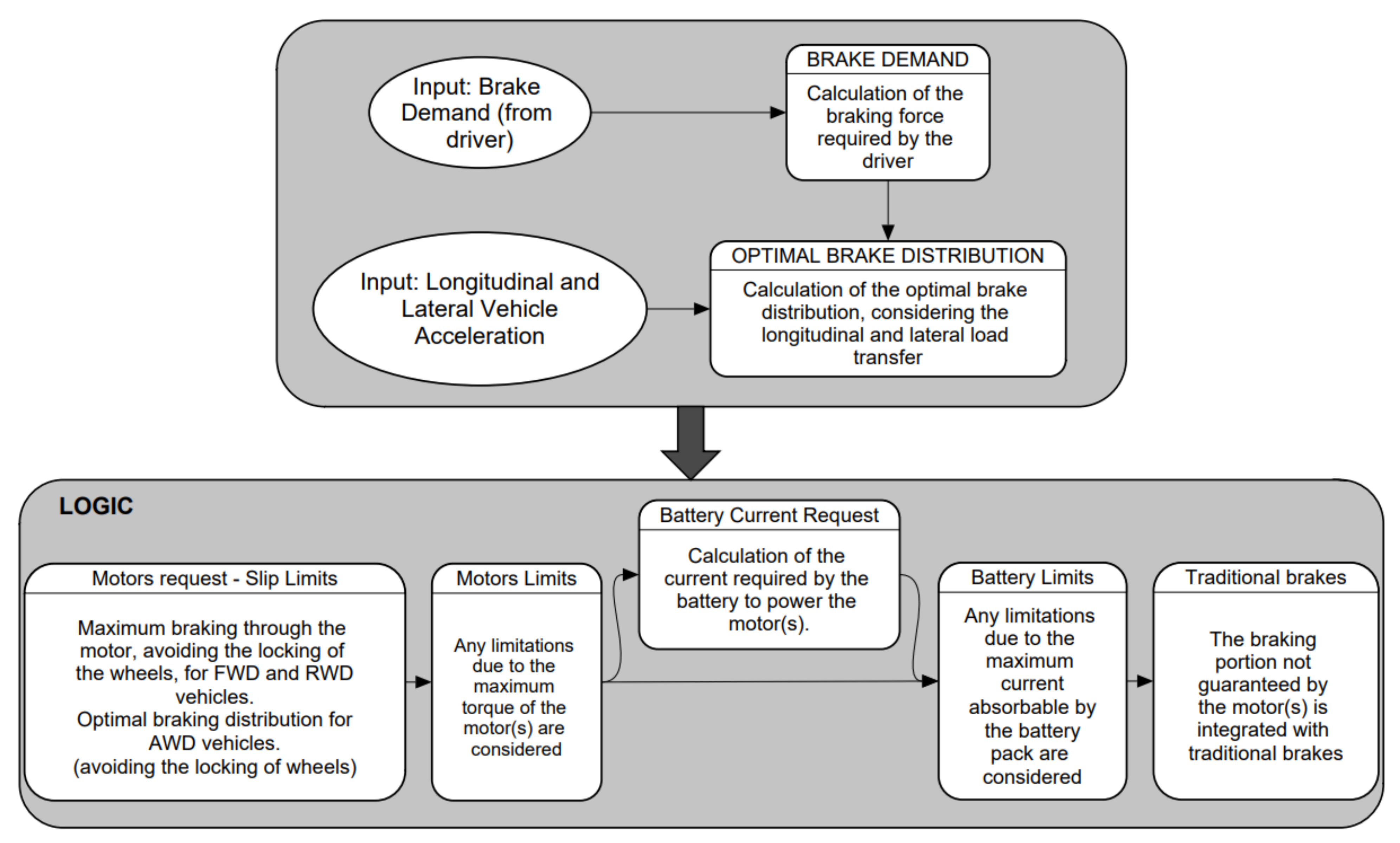

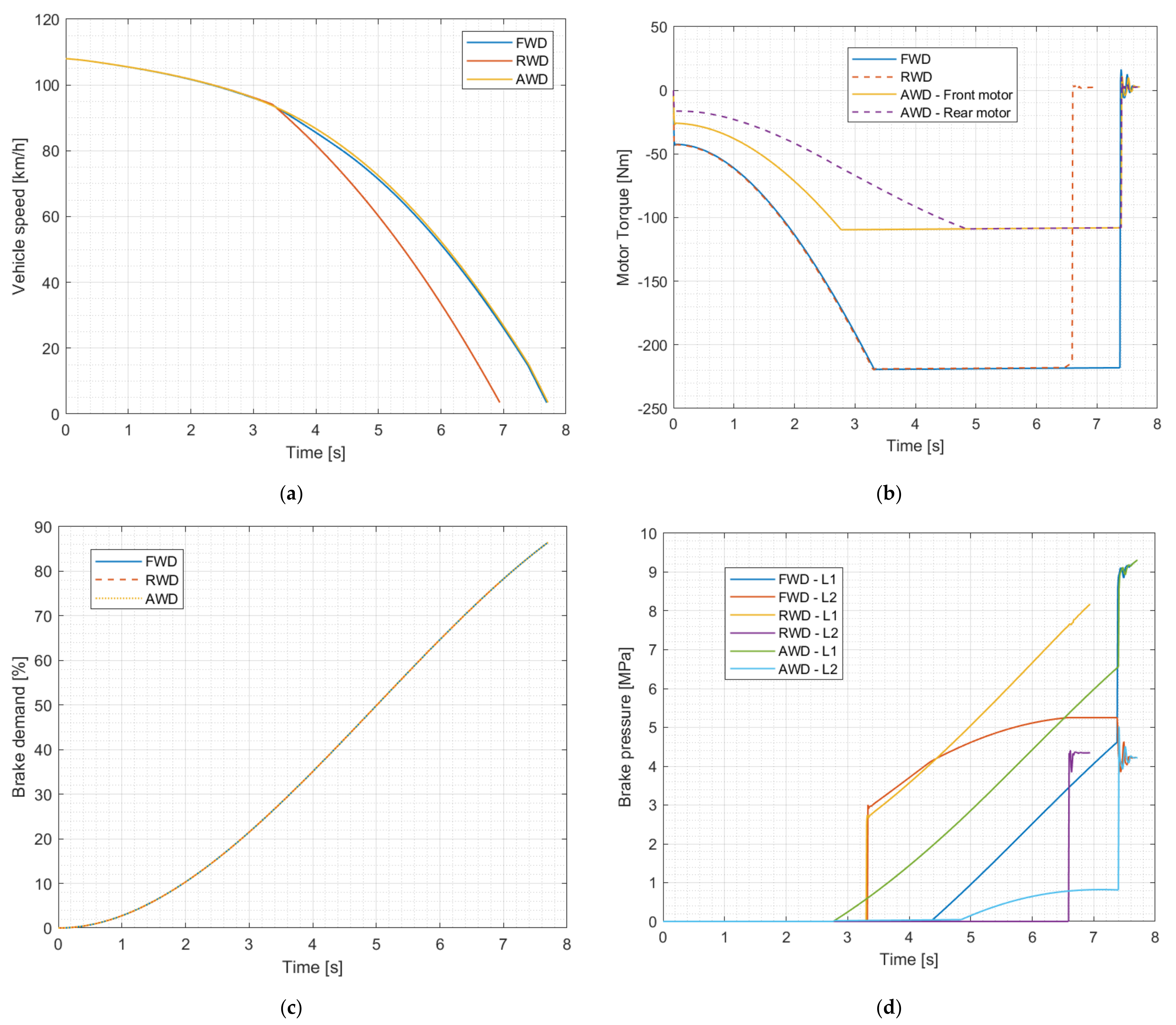
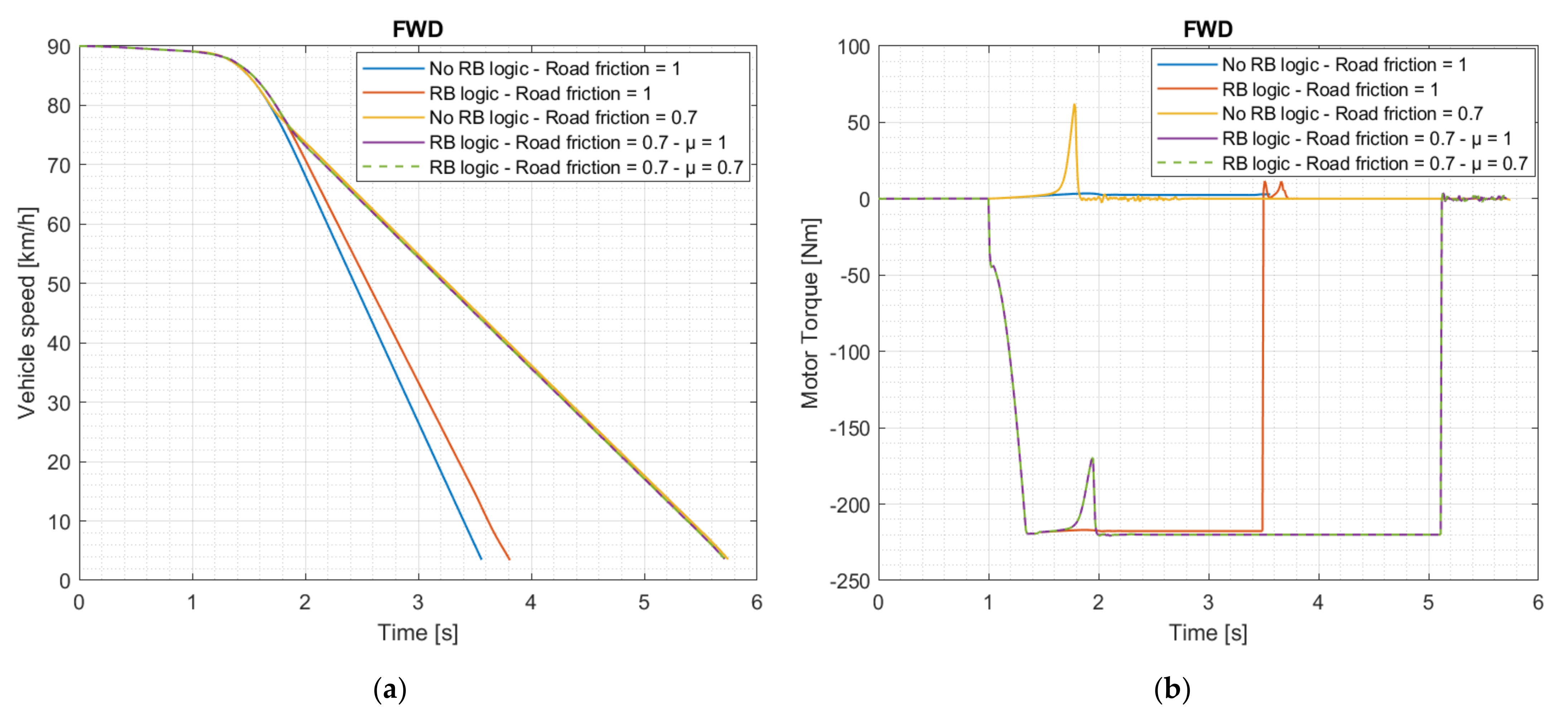
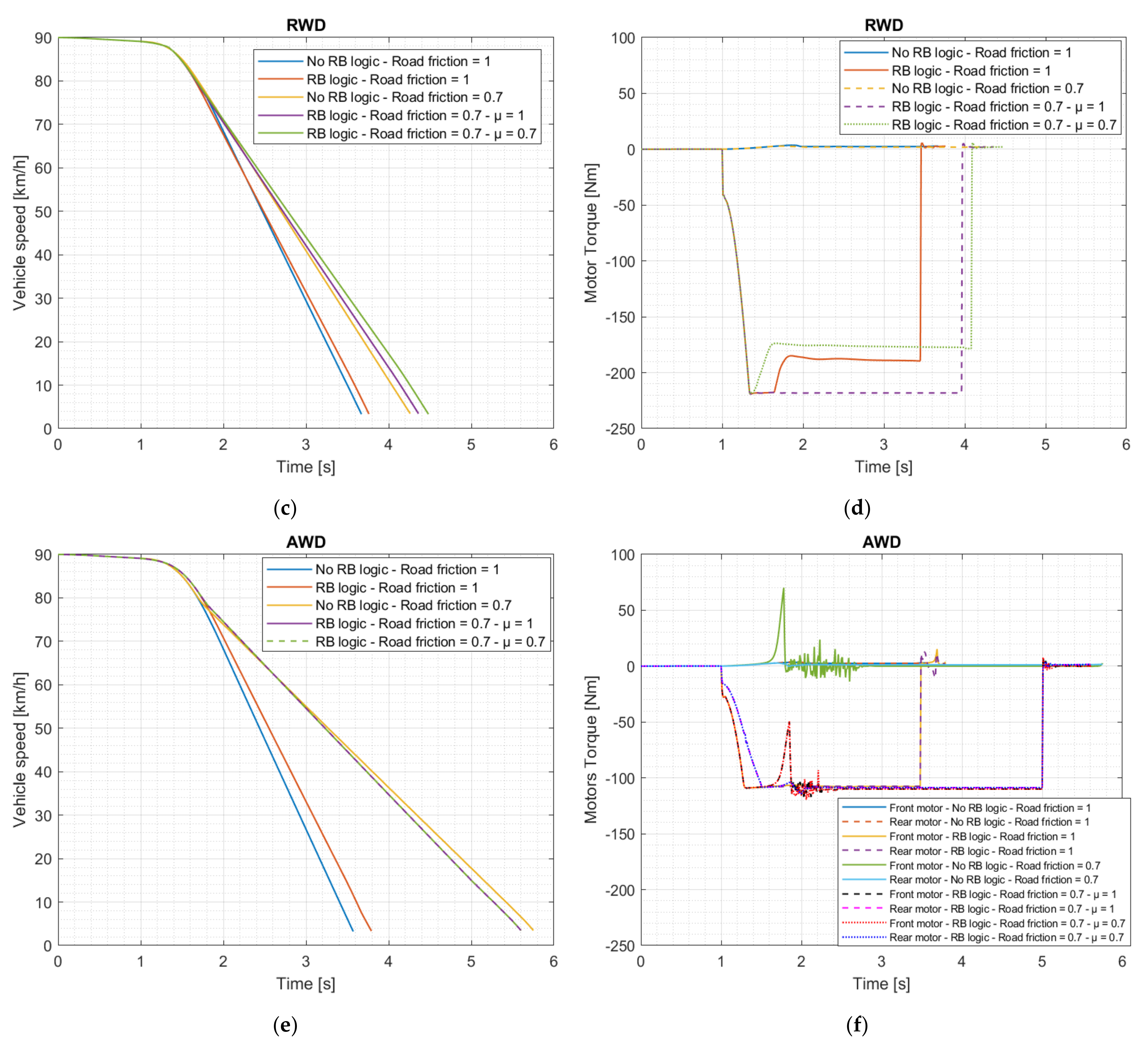
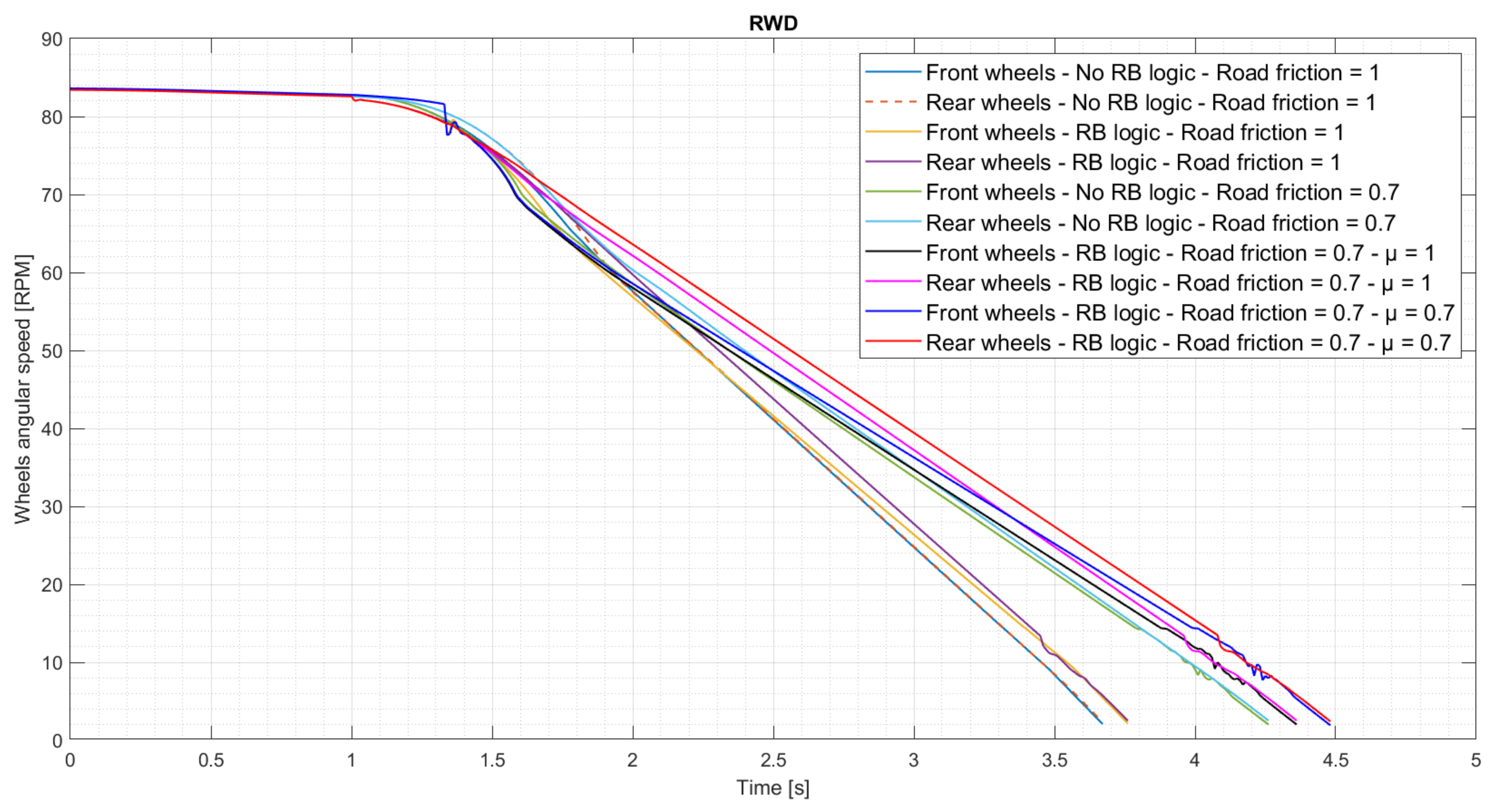
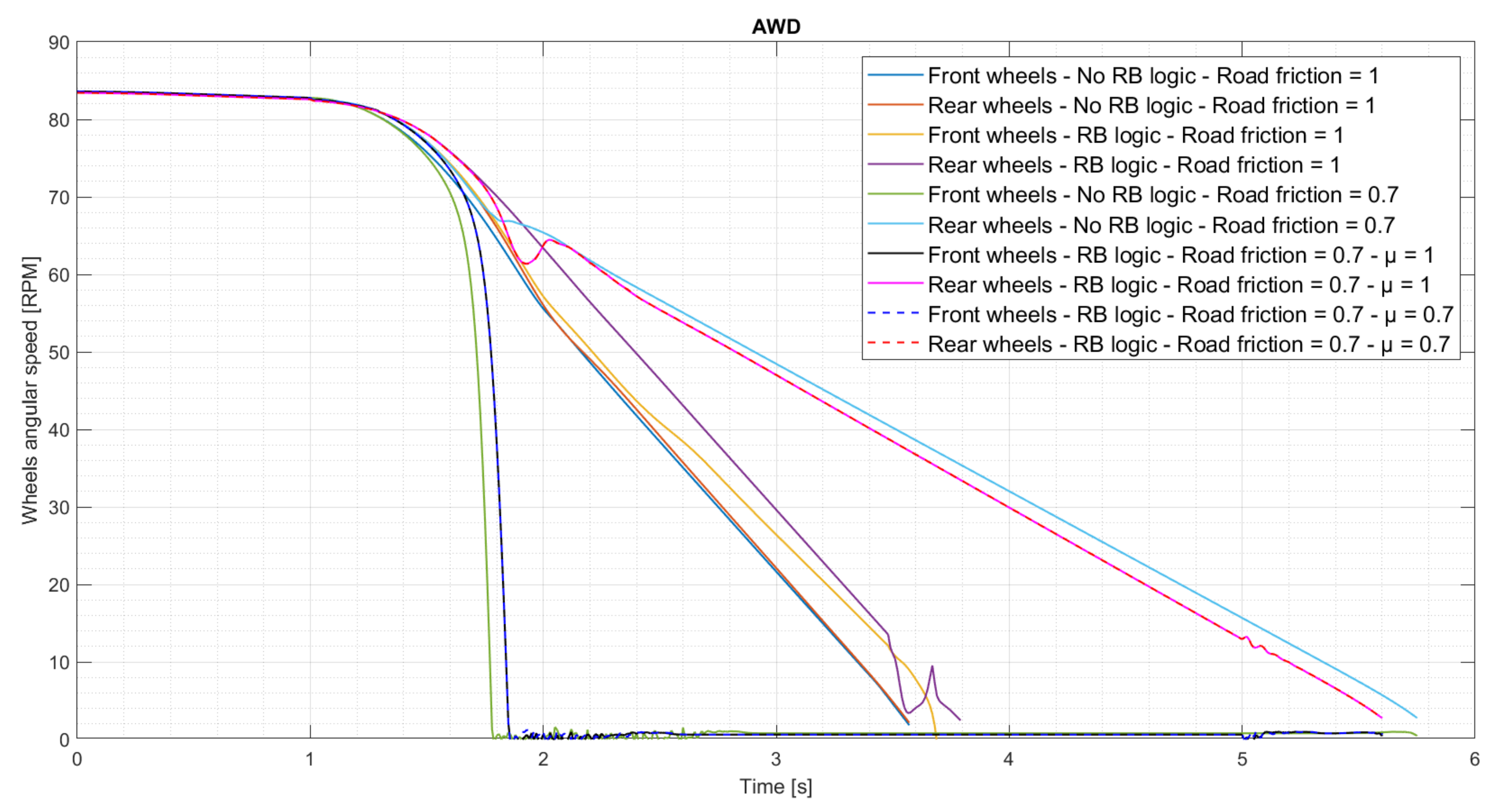
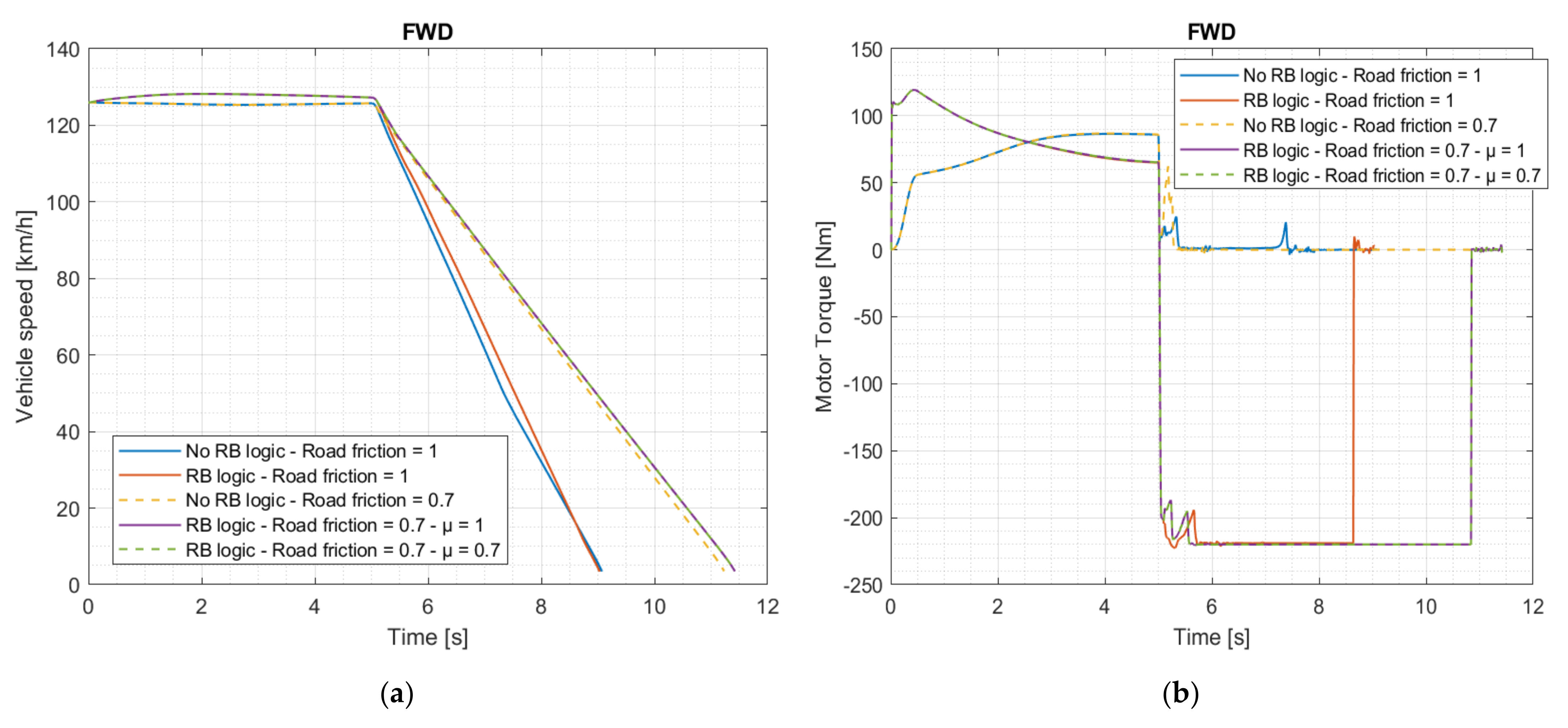
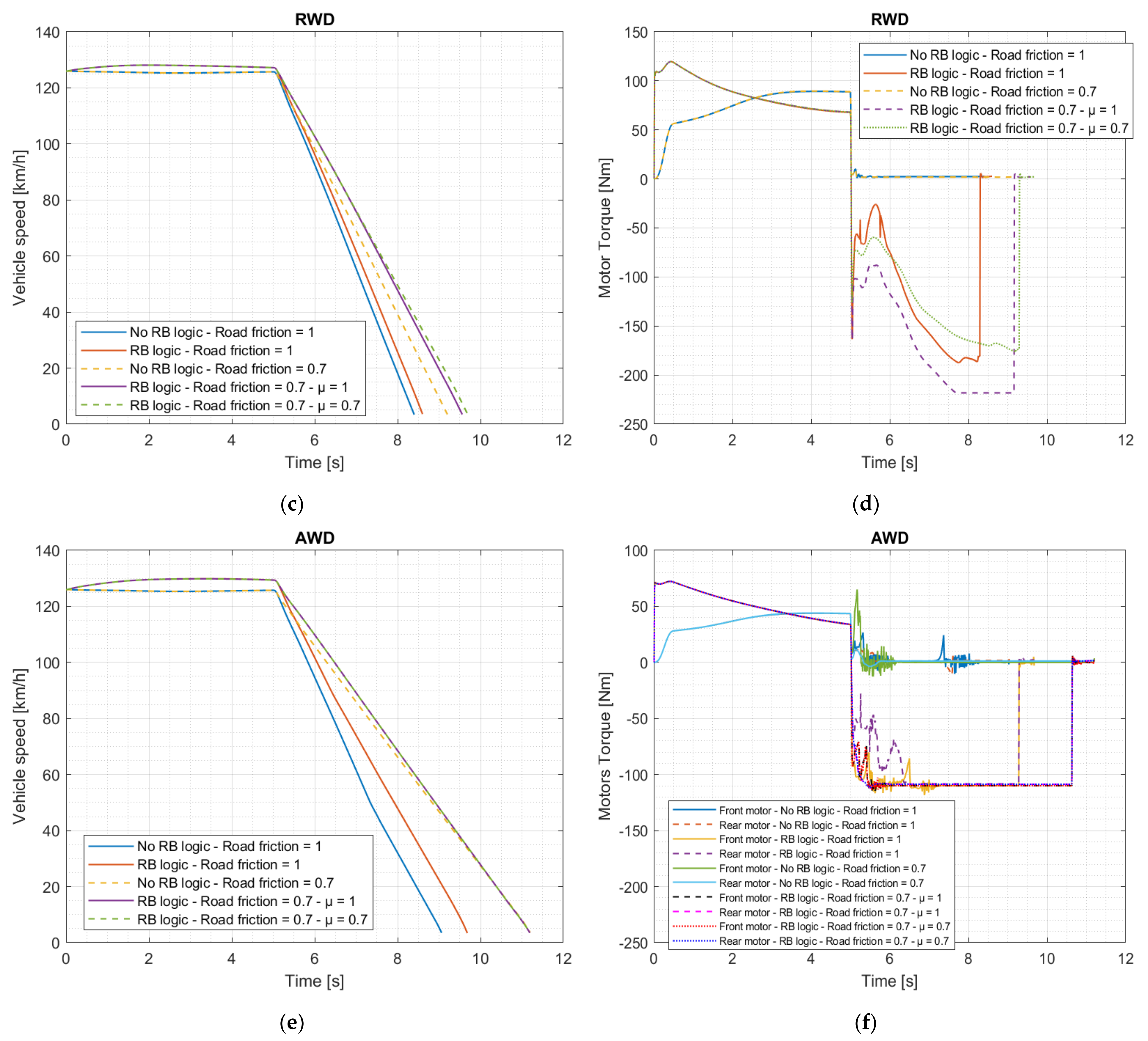
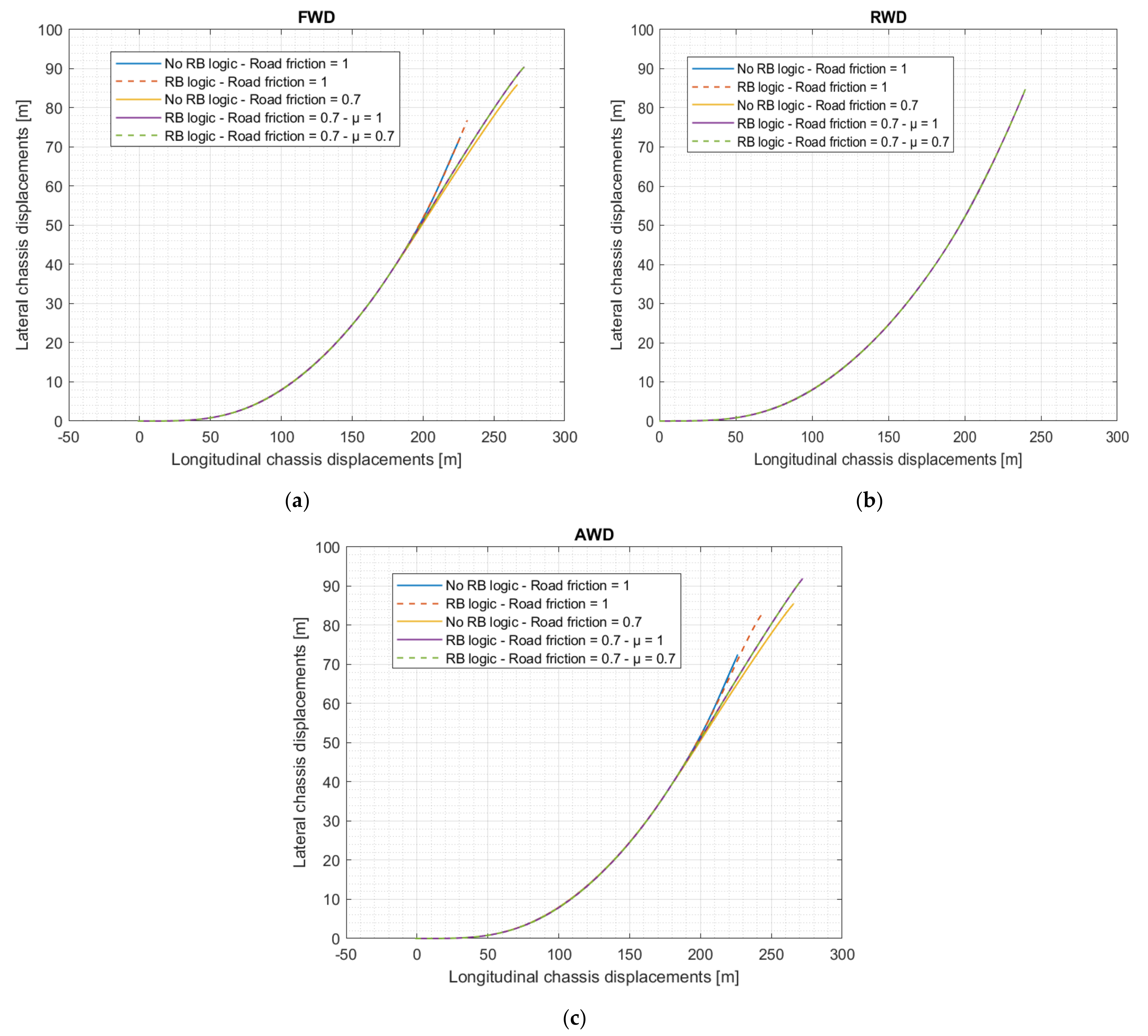
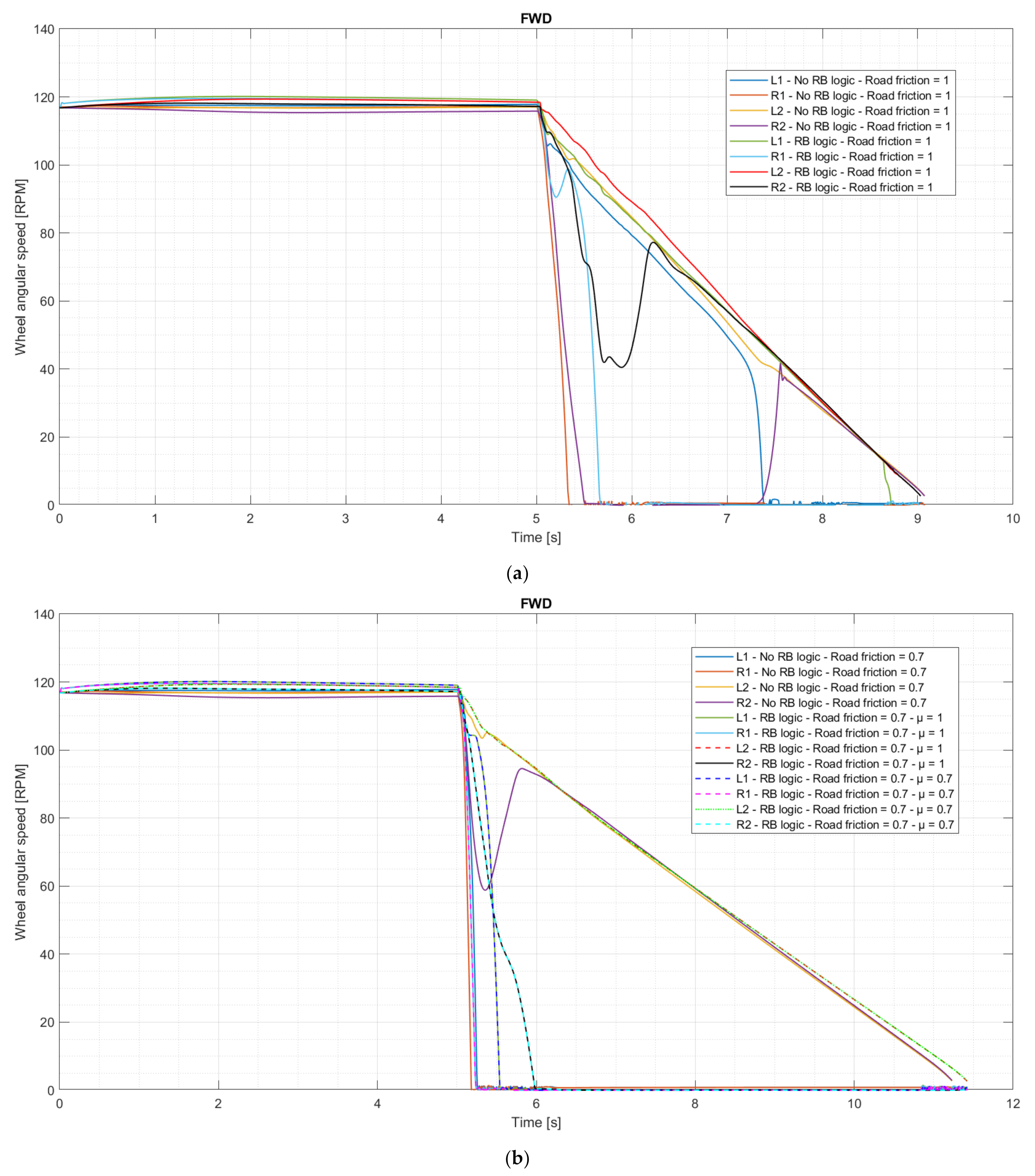
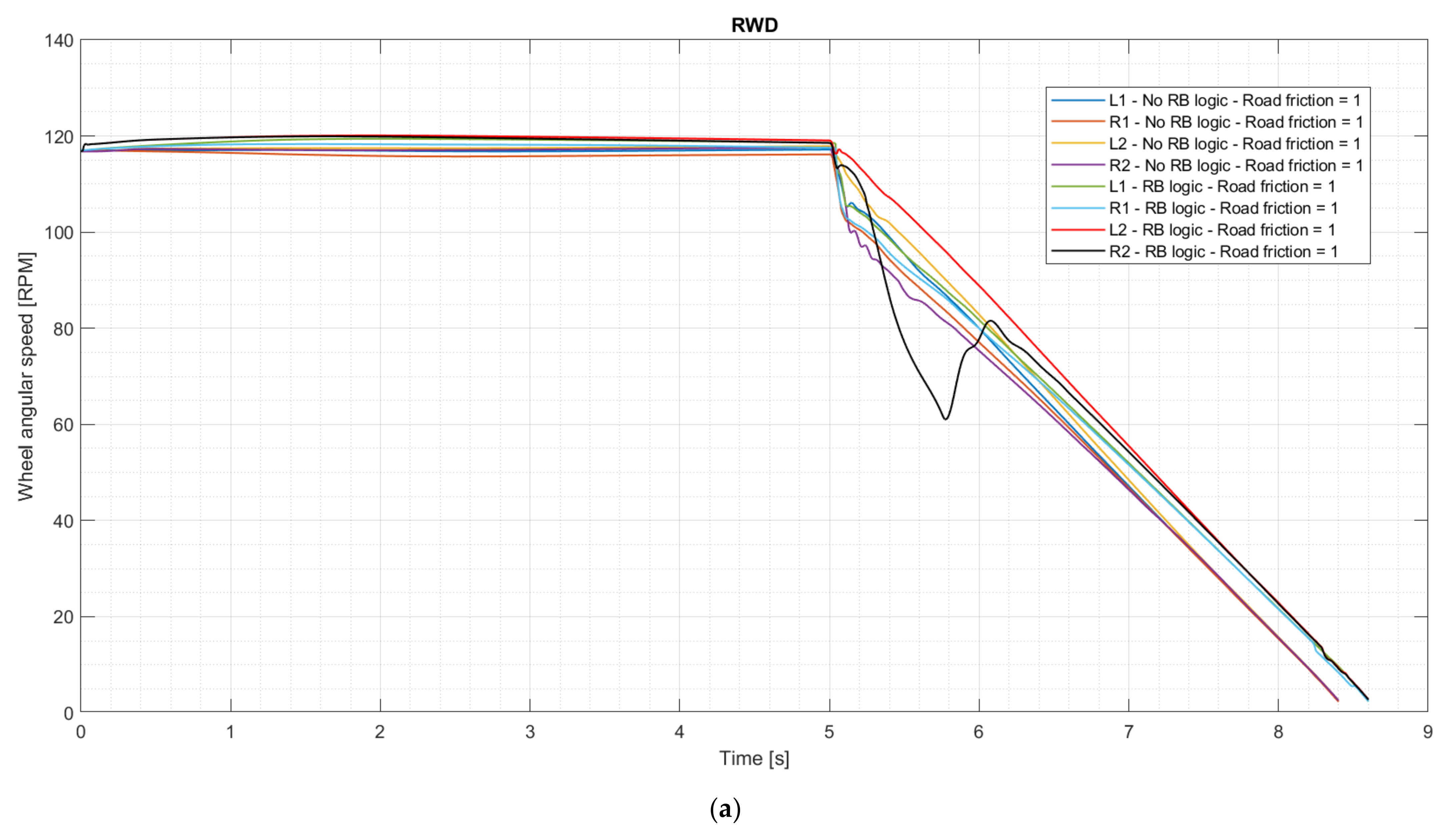
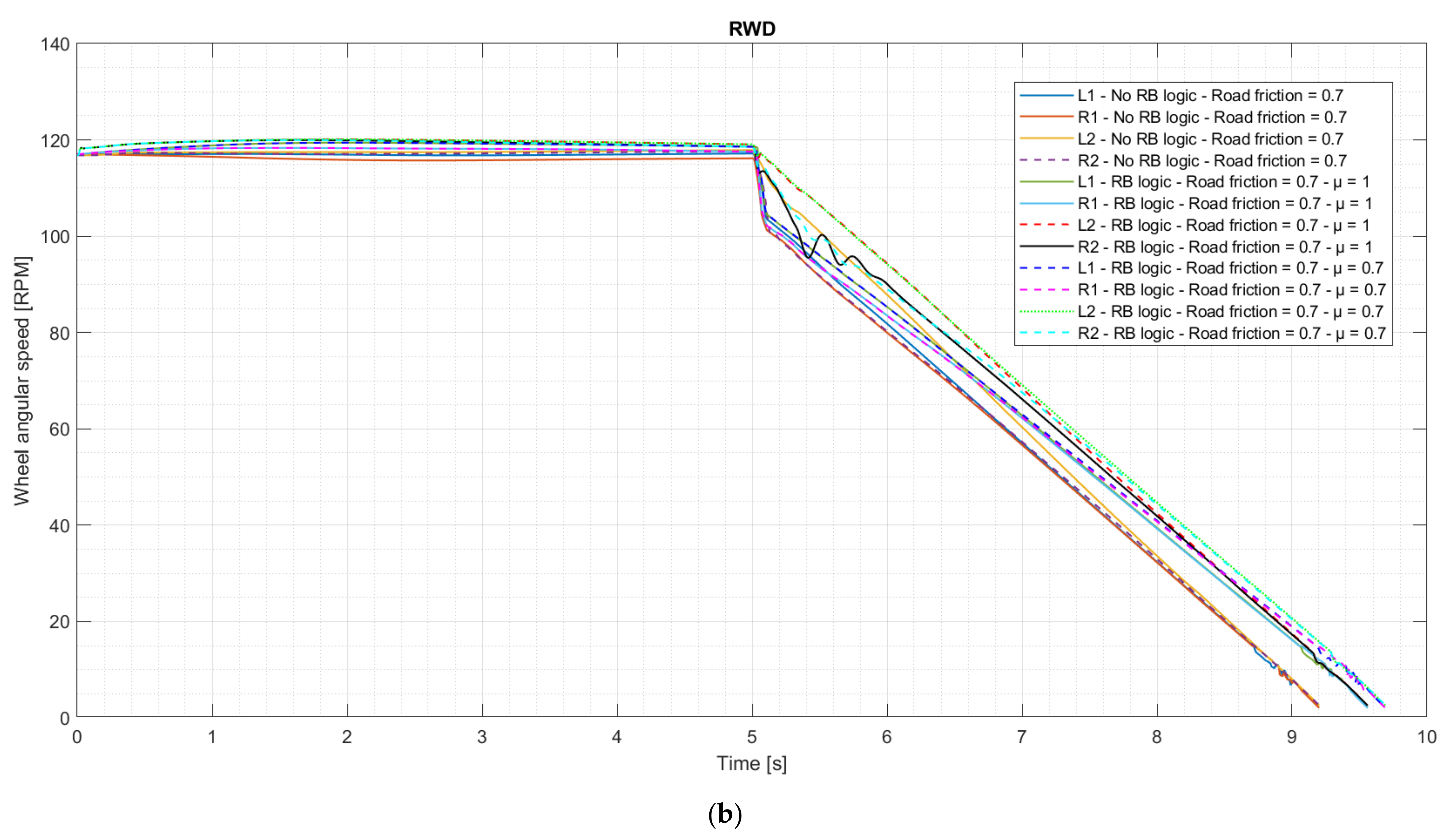
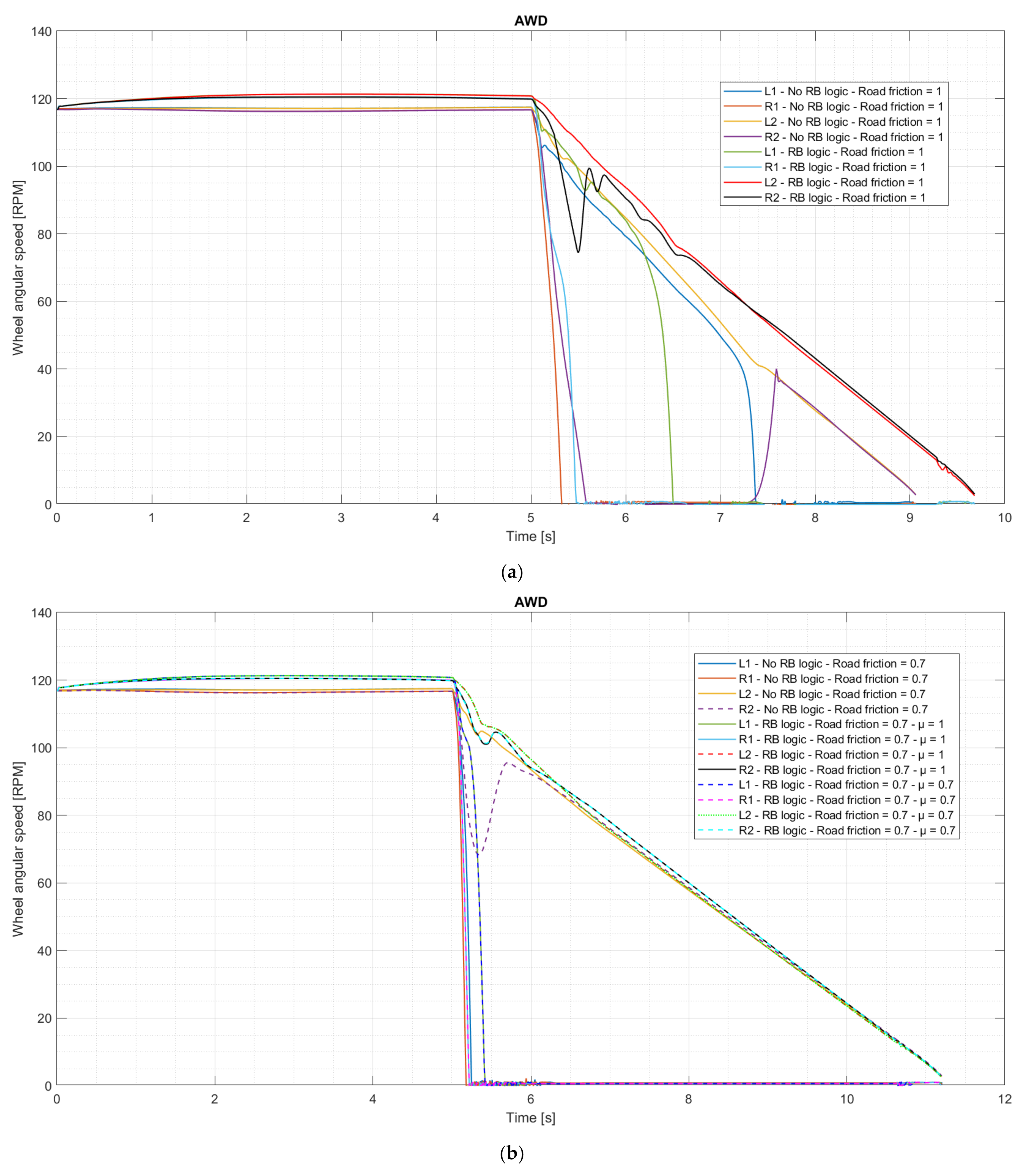
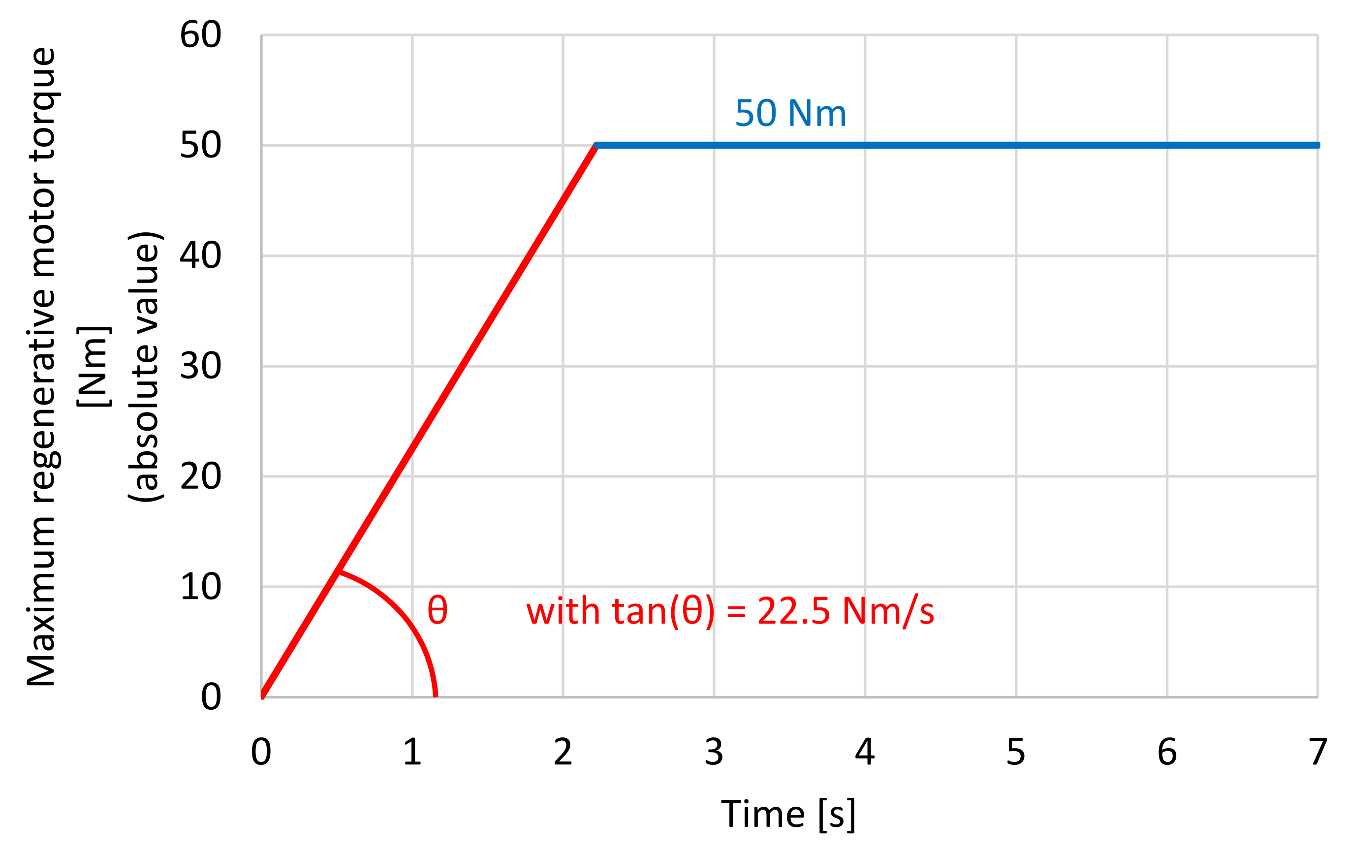
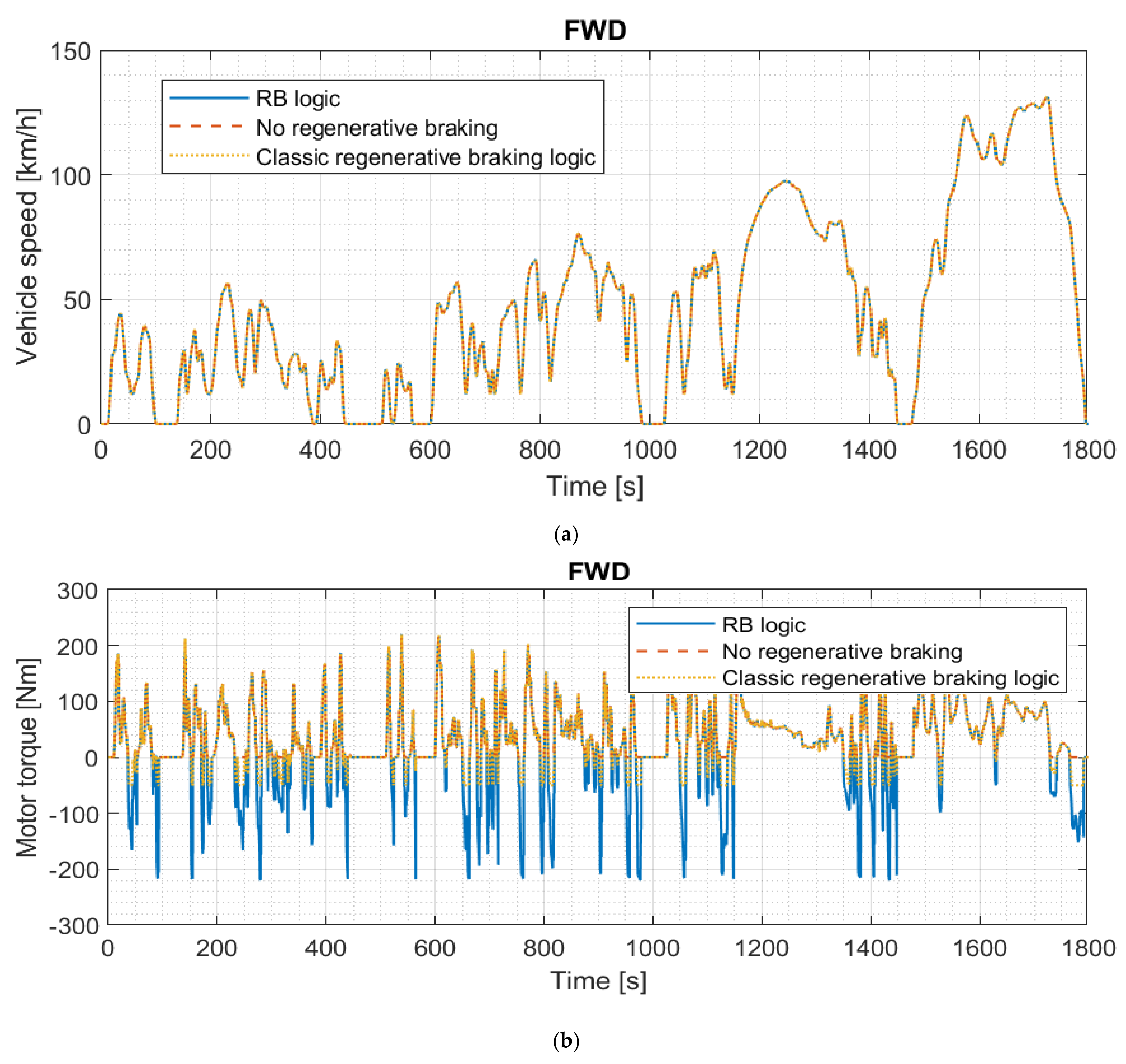
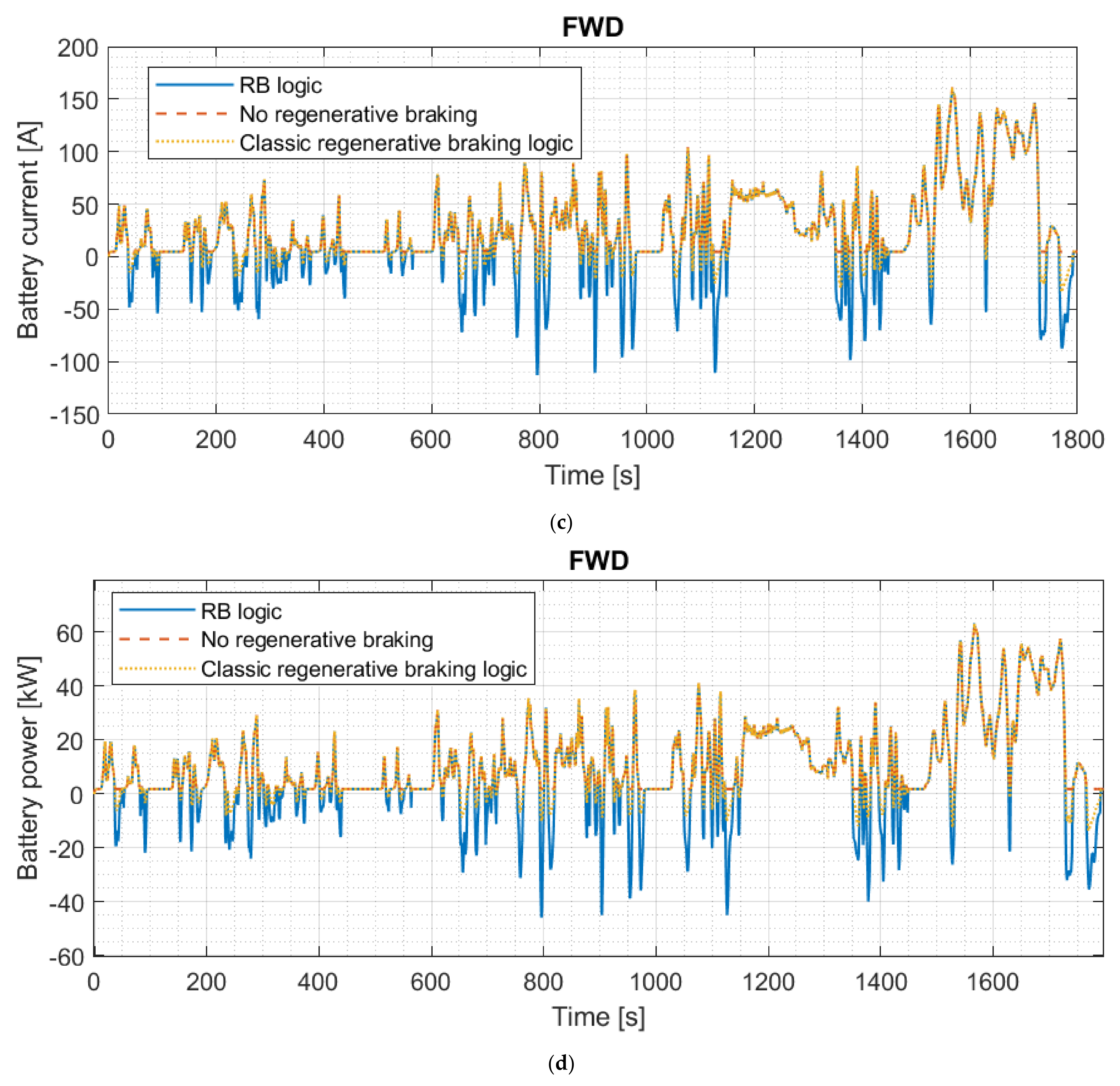
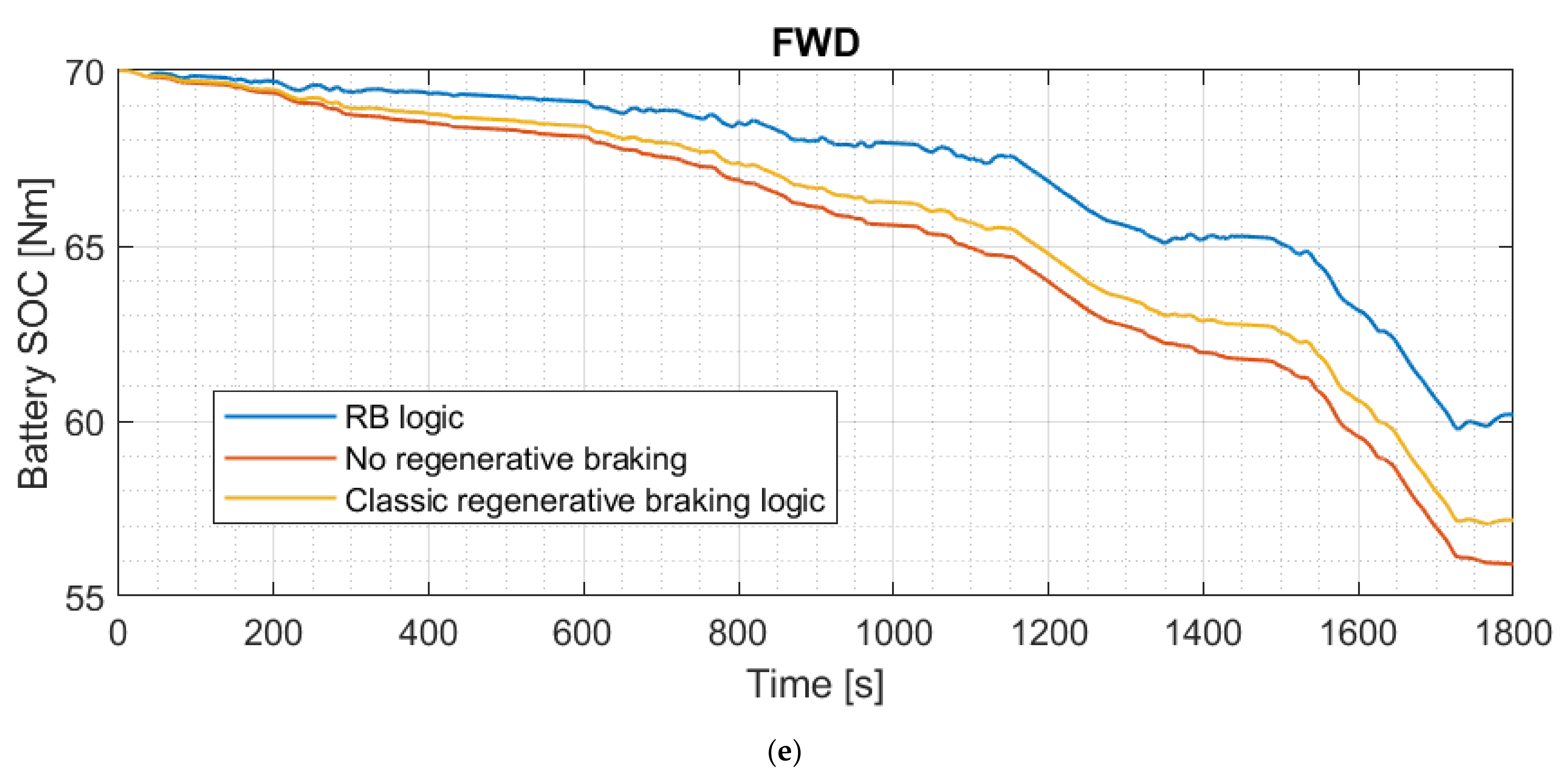
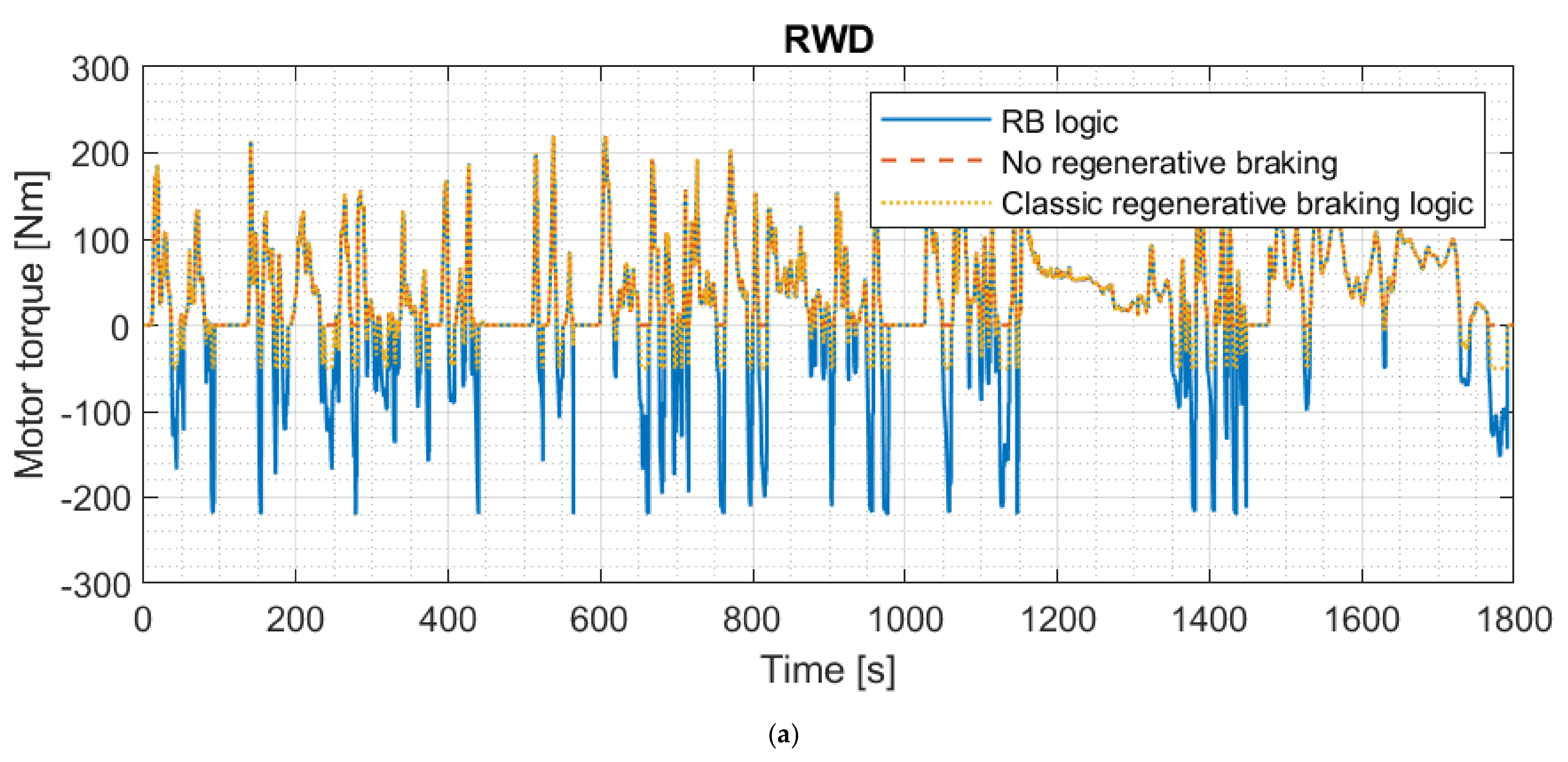
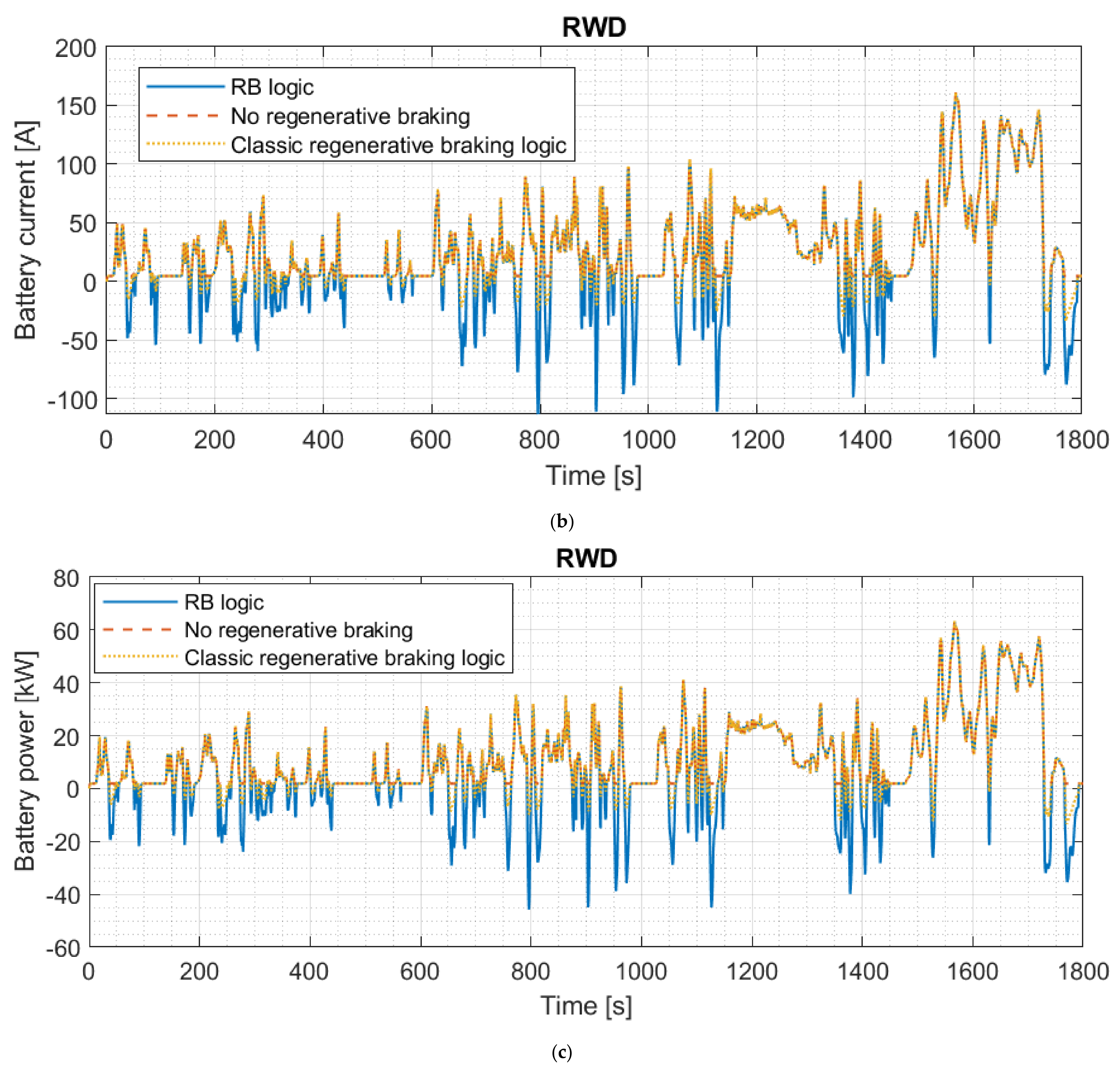
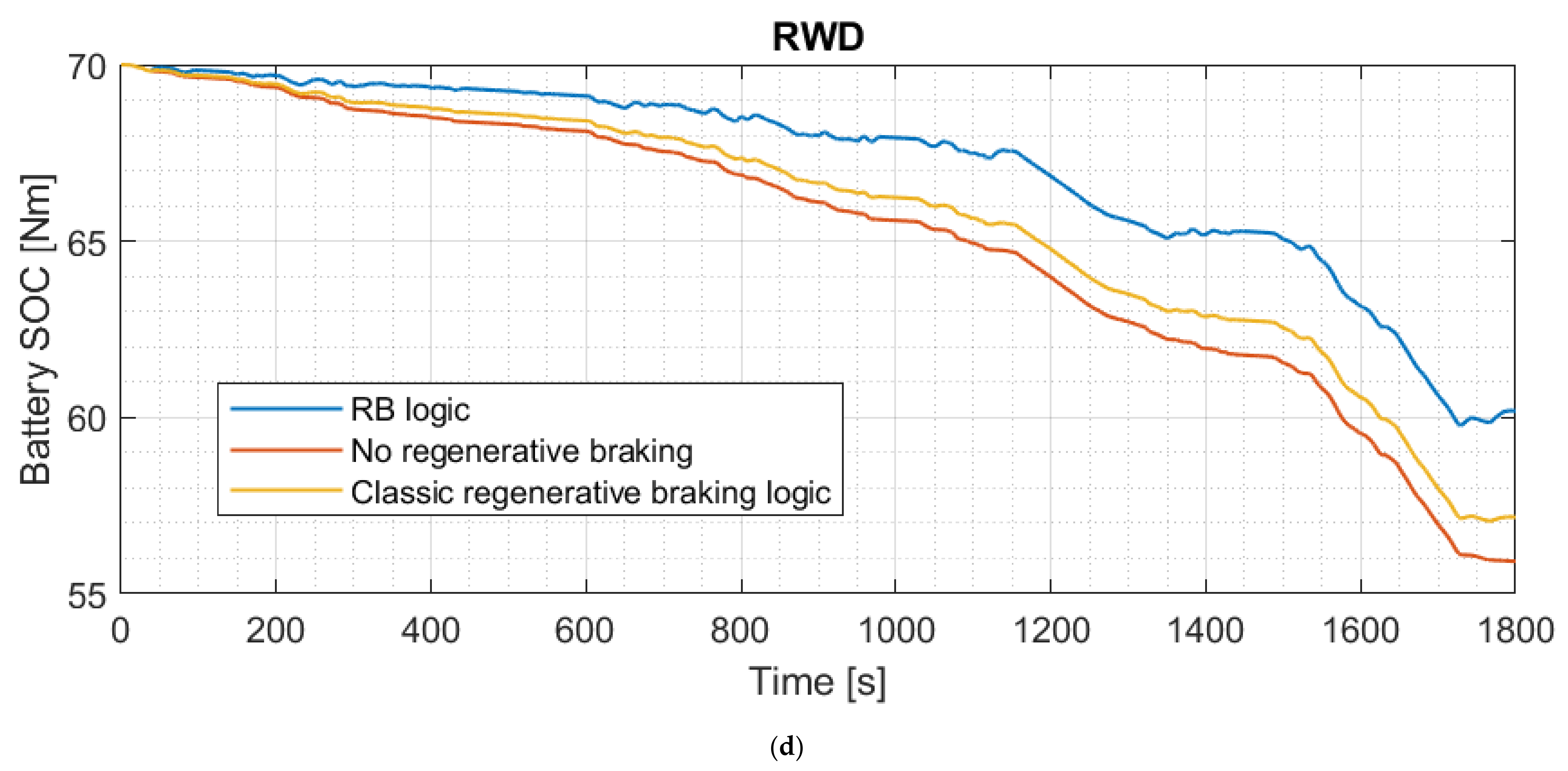
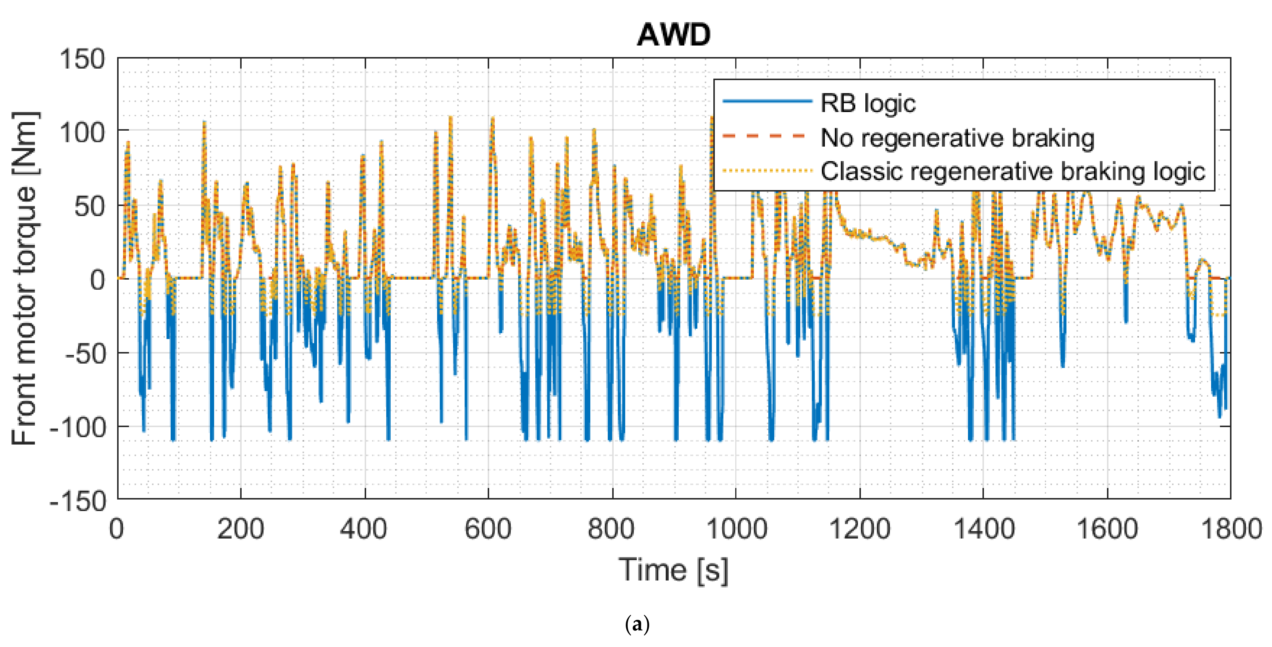
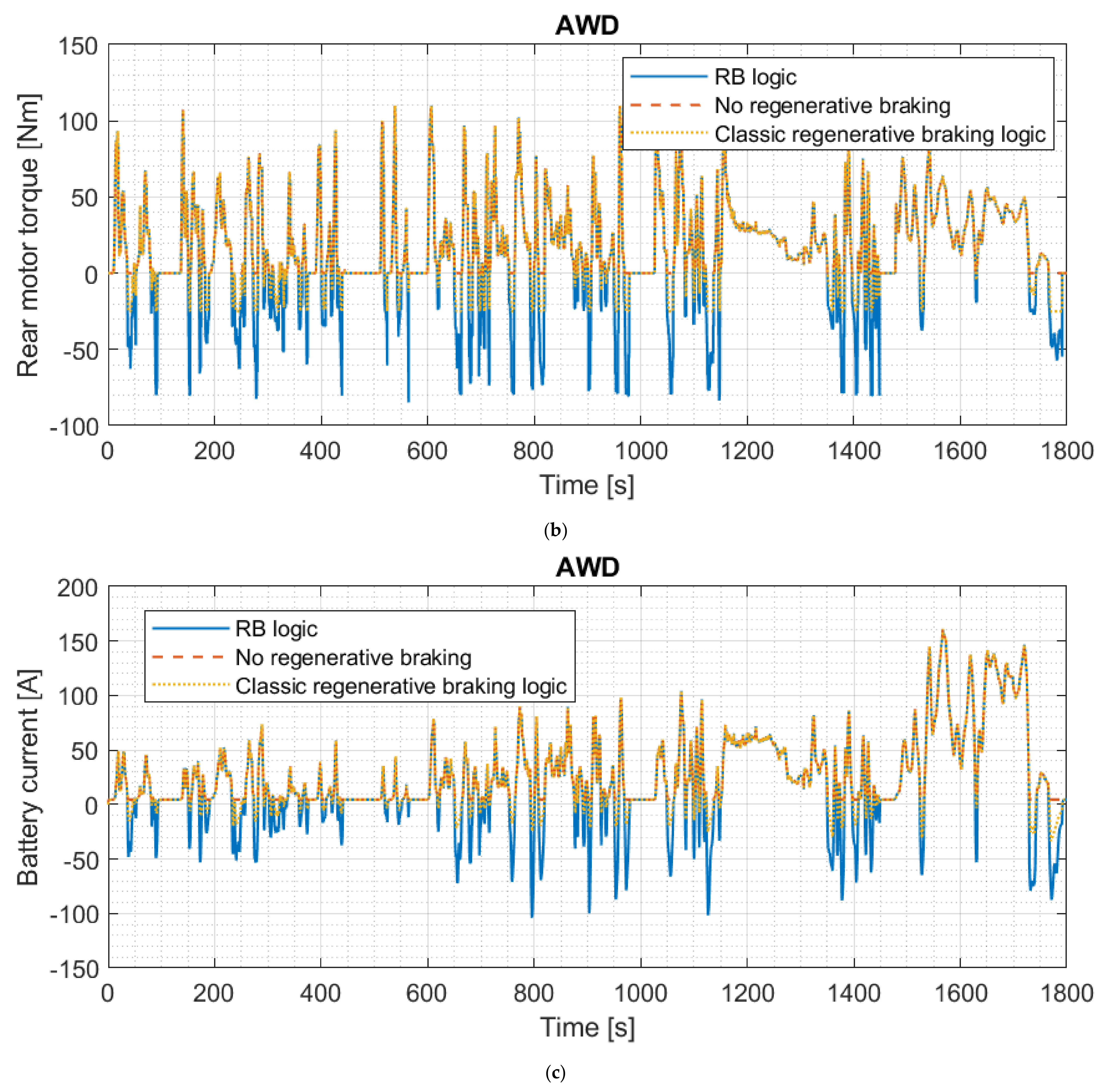
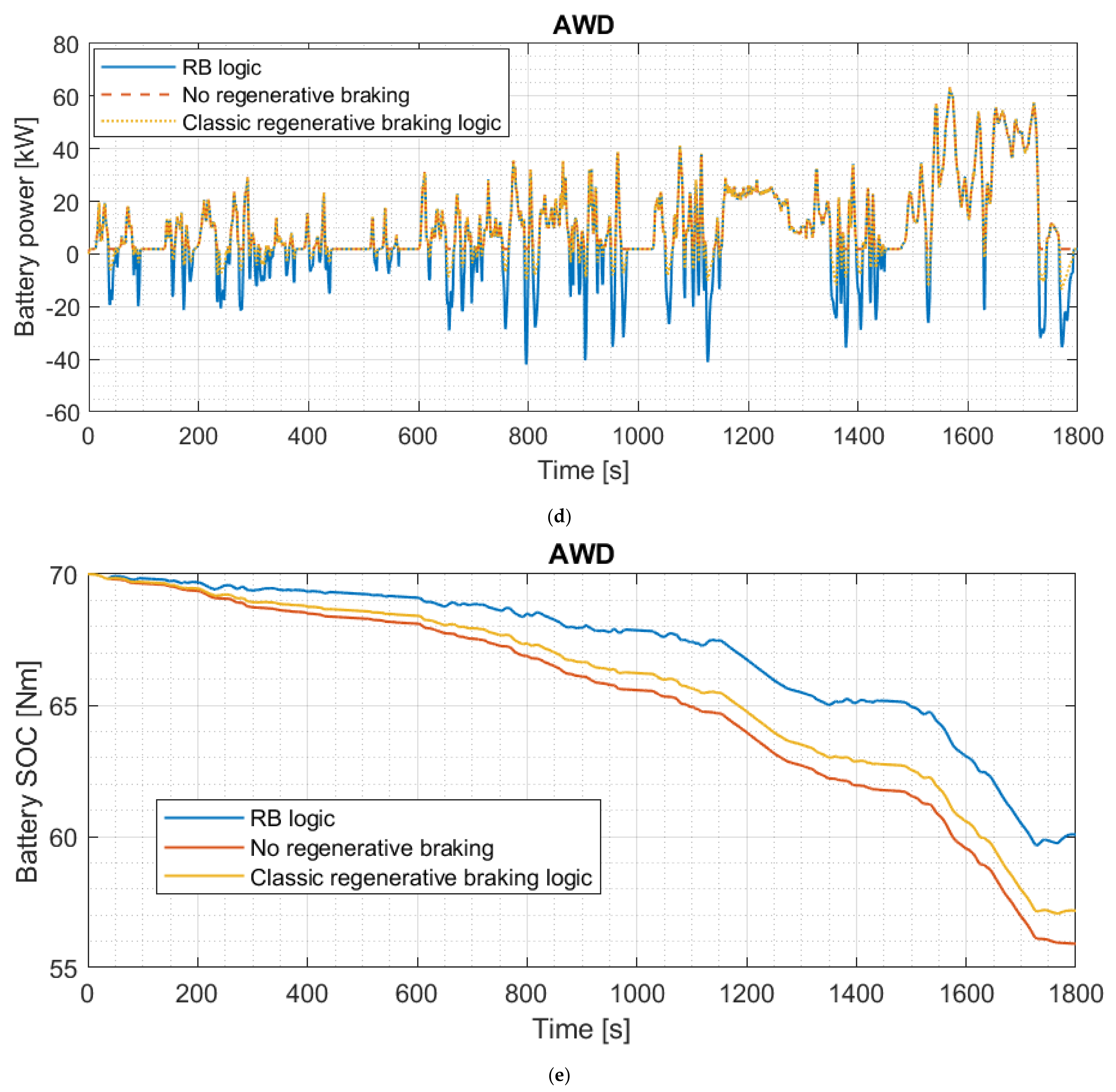
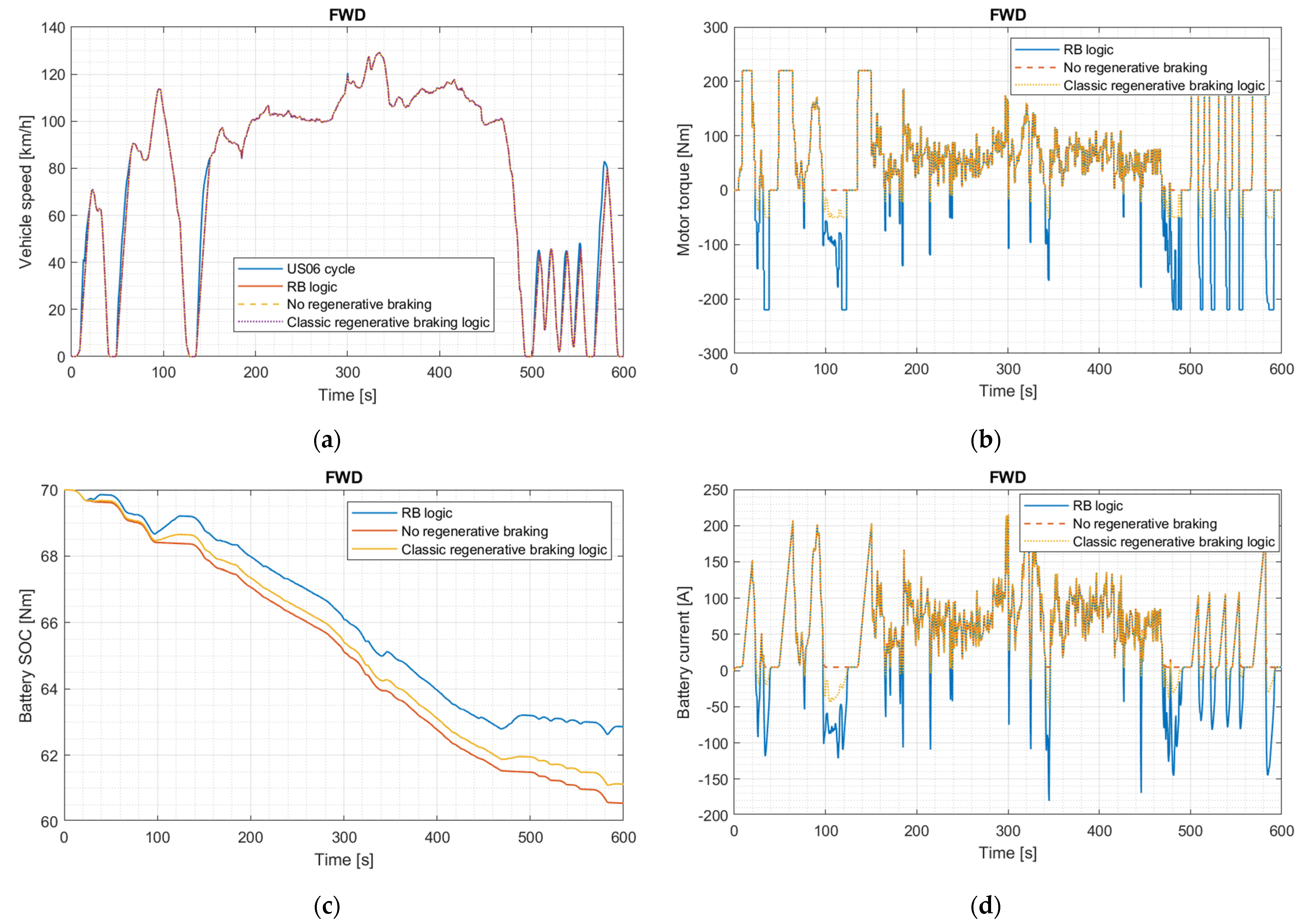
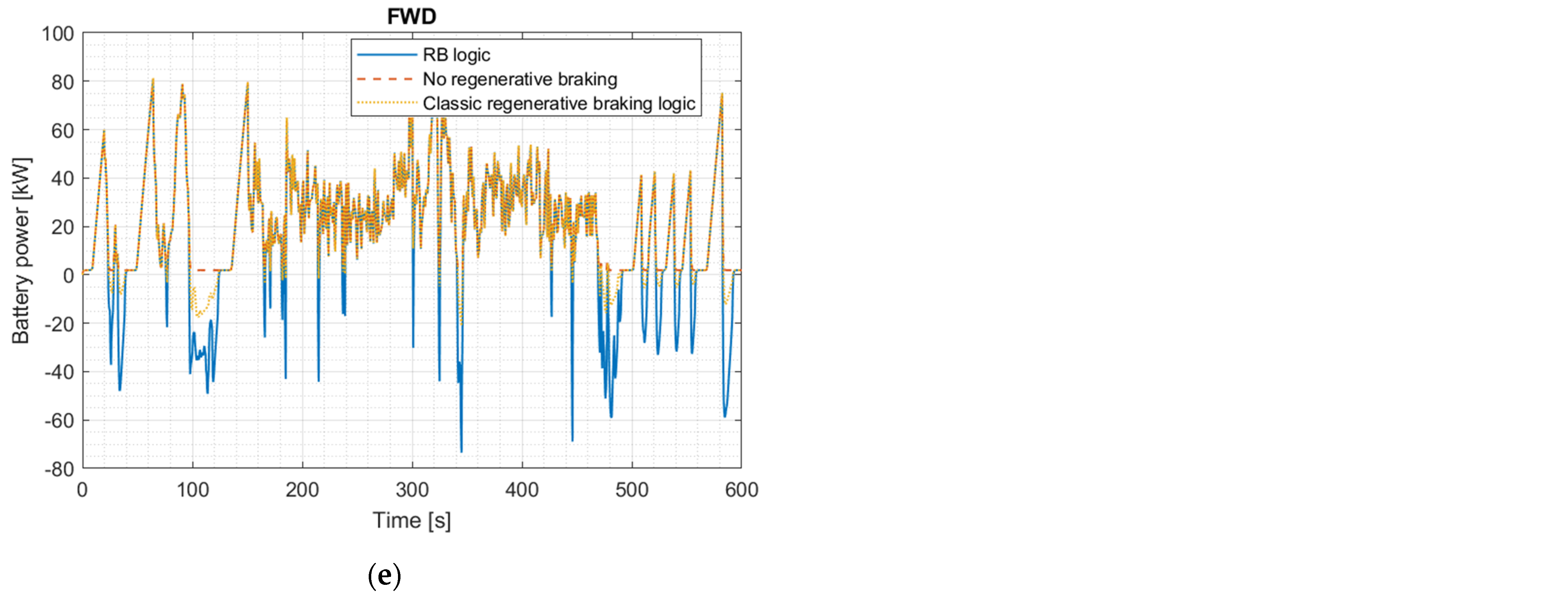
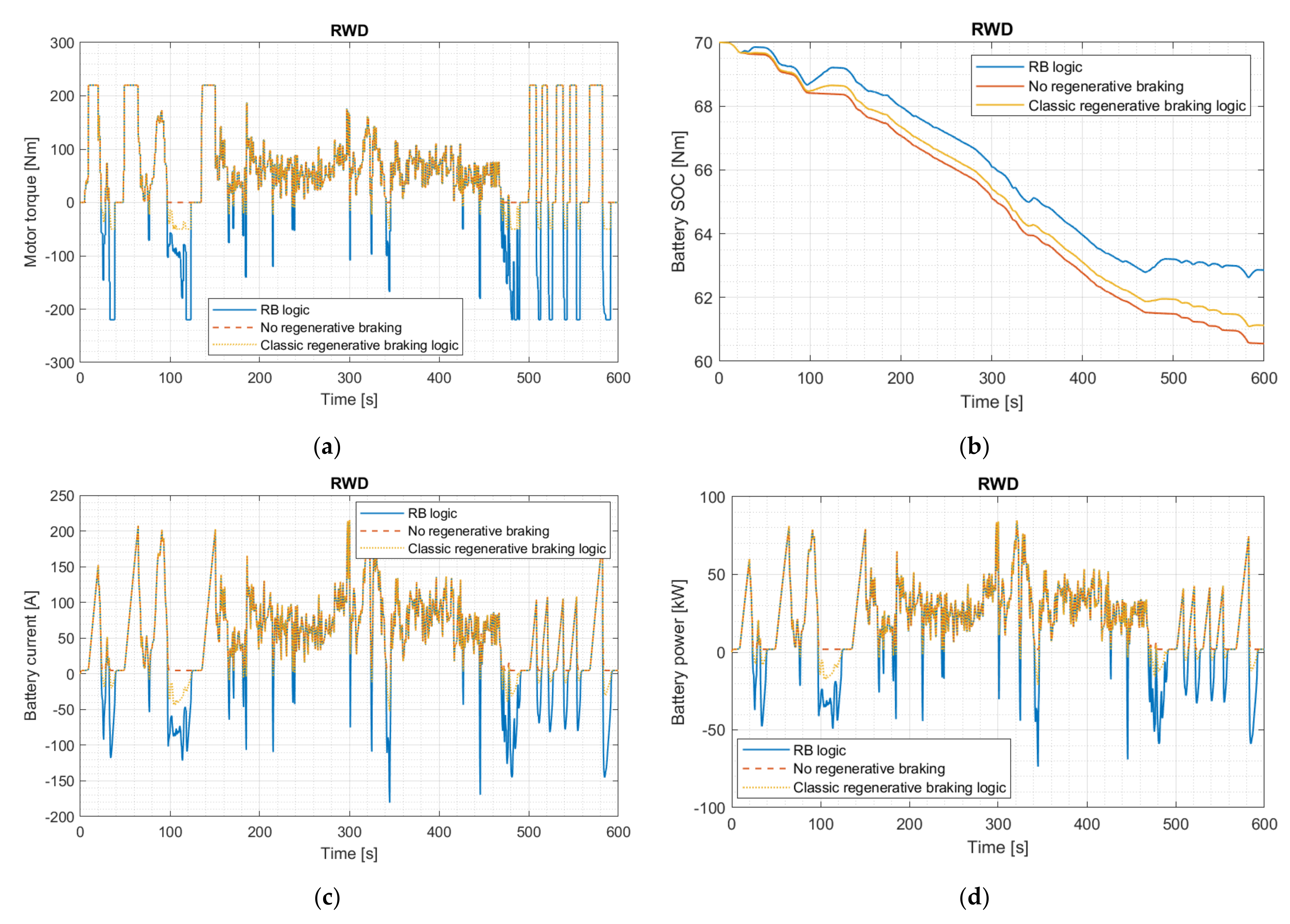
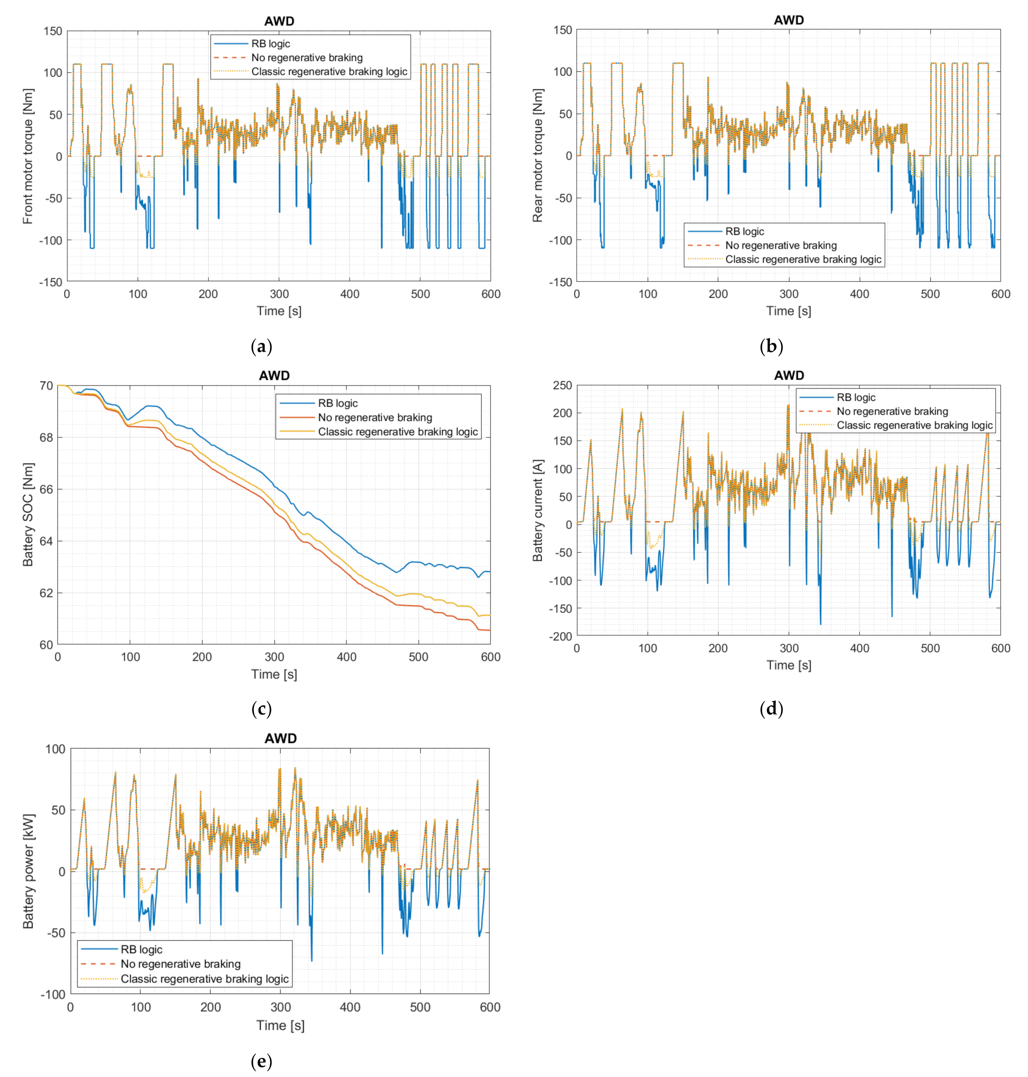
Publisher’s Note: MDPI stays neutral with regard to jurisdictional claims in published maps and institutional affiliations. |
© 2022 by the authors. Licensee MDPI, Basel, Switzerland. This article is an open access article distributed under the terms and conditions of the Creative Commons Attribution (CC BY) license (https://creativecommons.org/licenses/by/4.0/).