An Exponential Solvent Chamber Geometry for Modeling the VAPEX Process

Abstract

Accurate simulation of the VAPEX process relies heavily on precise modeling of the solvent chamber propagation. In the previously developed models, the solvent chamber possesses either a linear, circular, or parabolic shape. In this study, an exponential solvent chamber model was considered to represent the propagation of the chamber throughout the spreading and falling stages of the VAPEX process. The tuning parameters of the proposed model include the exponential function coefficient and the transition region thickness. These parameters are altered by employing a MATLAB-based Genetic Algorithm (GA) to minimize the error between determined and measured cumulative produced oil in four experimental case studies presented in the literature. According to the outcomes, the proposed method can accurately adjust the cumulative produced oil to the measured values in both spreading and falling stages. Additionally, the thickness of the transition region obtained by this model is in reasonable agreement with the laboratory measurements. Accordingly, the average relative errors of all four cases for cumulative produced oil and transition region thickness are 7.73% and 5.12%, respectively. Consequently, the model estimates the oil production rate with reasonable precision and the predicted solvent chamber shapes are well-aligned with the experimentally observed chambers.

1. Introduction

Vapor-Assisted Petroleum Extraction (VAPEX) is among the most effective solvent-based Enhanced Heavy Oil Recovery (EHOR) techniques when applied at the laboratory scale. In this method, vapor solvent is introduced into the reservoir via a horizontal injector. Due to the occurrence of molecular diffusion and convective dispersion, the introduced solvent dissolves into the heavy oil, primarily in the transition region, thereby reducing its viscosity. Finally, gravity helps the less viscous oil to travel through the transition region from the top of the solvent chamber towards a horizontal producer beneath the injector [1,2]. At the same time, the injected solvent propagates in both axial and lateral directions, replacing the produced oil to expand the solvent chamber. In this process, the solvent chamber propagates in three stages: rising, spreading, and falling. After establishing a connection between the well pair, the rising stage begins. This stage ends after the solvent chamber touches the peak of the experimental model. The spreading stage takes place when the solvent chamber expands sideways to reach two top corners at either end. The final stage expresses the movement of the solvent chamber alongside the sidewalls of the model [3].

The VAPEX process offers several benefits to the petroleum industry, making it attractive. In heavy oil reservoirs that possess thin and extra thin heights, VAPEX has demonstrated superior performance in comparison with other thermal-based techniques, mainly Steam Assisted Gravity Drainage (SAGD) and Cyclic Steam Stimulation (CSS) [4]. This is due to the fact that when the thermal methods are applied to the reservoirs with thin pay zones, a significant amount of steam energy is lost to the overburden and underburden formations. Consequently, these reservoirs are less suitable for thermal methods. Furthermore, this method consumes less energy than thermal methods since it takes place at reservoir temperature, rendering a more environmentally friendly process [5]. Moreover, in this process, asphaltene precipitation in the vicinity of the production well leads to in situ upgrading of the diluted oil [6], allowing higher quality oil to be produced. It should not be left unmentioned that the slow production of oil in VAPEX hampers its application in the field. However, a higher temperature solvent vapor injection can improve the field performance of VAPEX [7]. Additionally, similar to SAGD [8,9], VAPEX may be adversely affected by heterogeneities such as the presence of shale layers and porosity, in addition to permeability variations throughout the porous media. Consequently, these parameters may limit the growth of the chamber.

The simulation of the VAPEX process can be carried out through numerical approaches and analytical modeling. The numerical simulators require detailed sets of data which are both expensive and time-consuming. By comparison, analytical approaches with reasonable assumptions can provide reliable results with minimum input data. The following paragraphs discuss both previously developed theoretical models and some numerical studies conducted in the past.

In order to determine the heavy oil production rate during the VAPEX process, several theoretical models have been proposed. The first analytical model for estimating the constant heavy oil rate during the spreading stage of the VAPEX process was proposed by Butler and Mokrys [10]. According to their model, only the transition region can drain diluted heavy oil into the producer. Additionally, oil saturation within the transition region rapidly falls to its lowest level of residual oil saturation. Using cementation factors, Das and Butler [2] extended the Butler and Mokrys model to capture the influence of porous media. A correlation was developed by Yazdani and Maini [11] to translate laboratory-measured heavy oil production rates to field-scale production rates. As opposed to the Butler and Mokrys estimate of 0.5, their findings indicate that heavy oil drainage is directly related to drainage height by a power of around 1.15. It should be noted that these models can only be used to estimate the heavy oil production at the spreading stage of the VAPEX process. However, they are not able to evaluate the propagation of the solvent throughout the process [12].

Using a linear solvent chamber, Moghadam et al. [13] developed the first model to express how the solvent chamber propagates in the spreading and falling stages of the VAPEX process. According to their model, the solvent–bitumen transition region would be bounded by two straight lines of constant thickness. Moreover, they considered a constant velocity profile for the altered heavy oil within the transition region. The model is fairly accurate in estimating heavy oil production rates and solvent chamber propagation throughout the falling stage.

Later, Lin et al. [14] introduced the circular propagation of the chamber to anticipate the oil production rate. They assumed a constant thickness for the transition region and a constant velocity profile for the diluted heavy oil within the transition region. Their model showed a greater performance throughout the rising stage.

In a more recent work, Ma et al. [3] developed a model assuming the solvent chamber propagates in a parabolic shape. Their suggested model ignored the rising stage and assumed a fixed thickness for the transition region. Moreover, the diluted heavy oil was assumed to maintain a constant profile throughout the transition region.

In a subsequent study, Wang et al. [12] suggested a semi-analytical model to predict VAPEX. In this model, a piecewise linear profile is used to estimate the transition region, which is modified over time. Furthermore, they considered the major mechanisms active during VAPEX, including mass transfer, gravity drainage, surface renewal, and multiple phase flow. They stated that the concentration of solvent within the transition region increases at a slower rate at the bottom compared to the top. In the middle, however, the concentration remains fairly stable. Moreover, it was demonstrated that a stable heavy oil production rate would be dependent on the square root of the diffusion coefficient of the solvent in the heavy oil.

In addition to the theoretical models, several numerical simulators have been used to analyze the VAEPX processes. As part of their investigation into the mechanism of miscible solvents dissolving heavy oil, Cuthiell et al. [15] used CMG. With the inclusion of random variations in permeability and physical dispersion, their numerical simulations matched fingering features and the later displacement stage similar to VAPEX. In their numerical study, Nghiem et al. [16] reviewed the key characteristics of an equation-of-state compositional simulation needed to simulate VAPEX. In addition to the molecular diffusion and convective dispersion, this simulation includes asphaltene precipitation and fluid mixing. The effect of different dispersivity coefficients on fluid mixing and chamber growth was also examined. Nourozieh et al. [17] proposed a three-phase flow within an individual grid block for VAPEX. A new phase for the solvent was added to the simulator to ensure a more accurate simulation of this process. Their model incorporates two separate spaces within one grid to simulate diluted bitumen and bitumen in separate grids. Since the boundary layer can be captured within a grid block, small grid blocks are not required for the transition zone. A study by Yazdani et al. [18] found some inherent pitfalls in the numerical modeling of VAPEX experiments. They mentioned that two sets of challenges must be overcome: one dealing with the limitations of simulators in modeling the lab-scale experiments and the other dealing with numerical methods.

This study sought to establish a novel theoretical model that is able to accurately evaluate solvent chamber propagation. In this newly developed model, the solvent chamber maintains an exponential geometry throughout the whole process. The proposed model also predicts heavy oil drainage within the spreading and falling stages of the VAPEX process. This model assumes a constant thickness for the transition region of the solvent and heavy oil during the whole process. By minimizing the discrepancies between the measured and determined cumulative produced oil, the thickness of the transition region can be determined. In addition to estimating cumulative oil production and solvent chamber propagation, the proposed model can estimate oil production throughout the entire process. Additionally, the performance of the proposed model was evaluated by comparing the results with those from four experimental cases conducted by Ma et al. [3], in addition to their theoretical model.

2. Materials and Methods

Based on a previously developed model by Ma et al. [3], the equations of the proposed model were derived using the following assumptions:

• Solvent chamber possesses an exponential geometry throughout the process. Figure 1 and Figure 2 illustrate exponential propagation of the solvent chamber in concave and convex shapes, respectively.
• The transition region is constant in thickness during the whole process.
• Oil saturation within the transition region rapidly falls to its minimum value of residual oil saturation.
• The physical model is homogenous and isotropic.
• The diluted heavy oil within the transition region moves at its maximum velocity.
• Temperature and pressure remain constant throughout the process.
• There is no driving force for moving oil inside the transition region other than the gravity drainage.
• The rising stage is ignored as it was mentioned in the literature that this stage would contribute only 3% and 5% of the VAPEX process time and oil recovery, respectively [3,14].

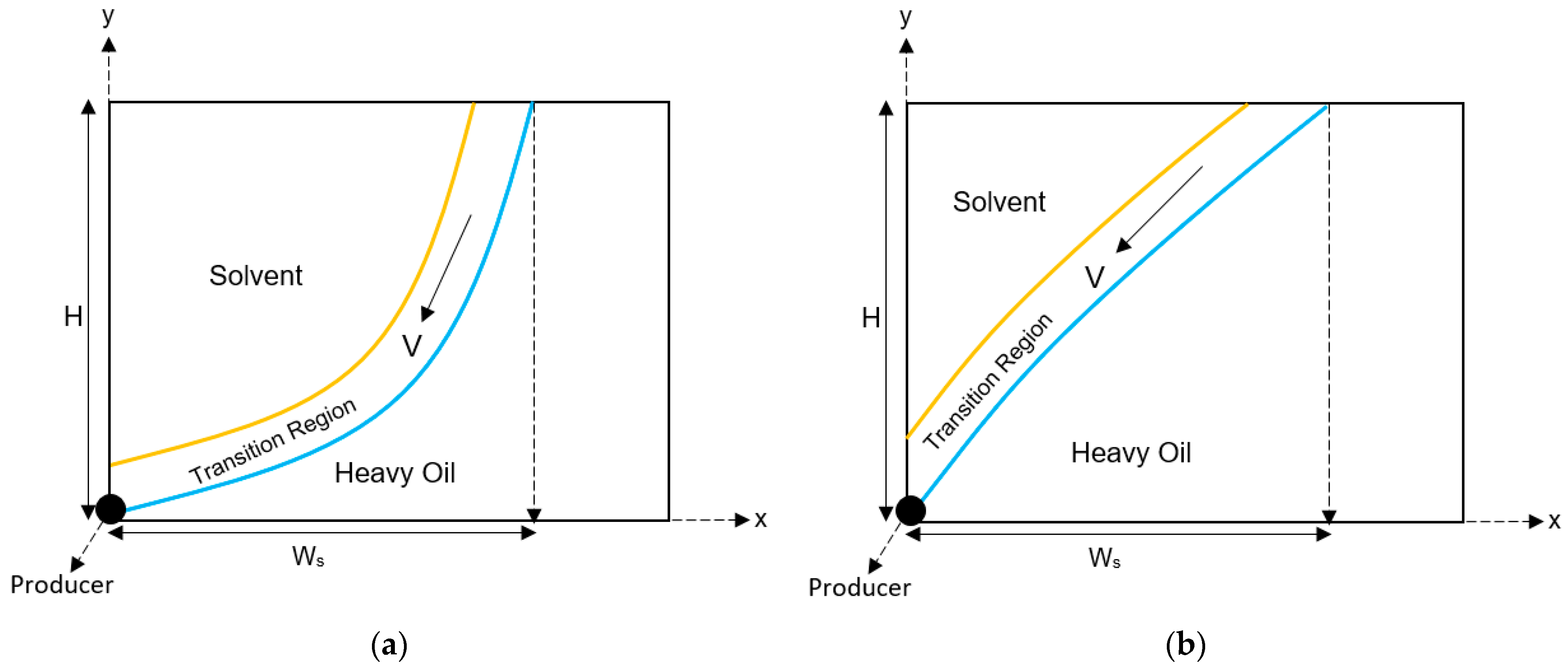
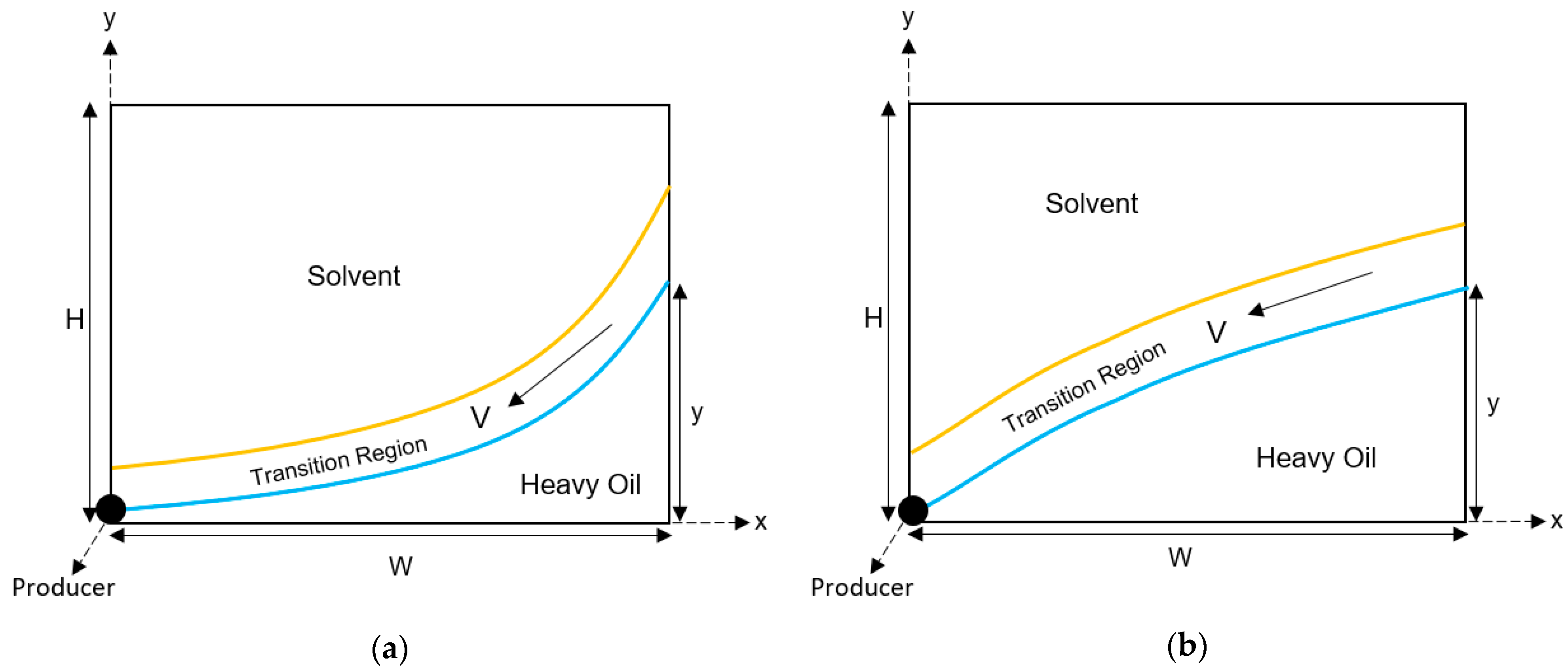
2.1. Mathematical Modeling of the Rising Stage

In order to describe the solvent chamber propagation during the spreading stage, and with the producer at the origin, Equations (1) and (2) can be used for concave and convex cases, respectively:

$$y=a\times \left(e^{nx}-1\right)$$

(1)

$$y=a\times \left(1-e^{-nx}\right)$$

(2)

where a is the time-dependent parameter showing the lateral spreading of the chamber and n is an adjustment parameter. In addition, y and x are the vertical and horizontal distances of the top of the solvent chamber form the producer, respectively.

Optimized values of a and n leads to an accurate simulation of the chamber propagation. It is therefore imperative to develop a formula that is capable of obtaining the values of a at any time in both concave and convex cases. Moreover, by minimizing the discrepancy between calculated and measured values for total oil production, the optimum values of n can be determined for these two cases.

Figure 3 illustrates the interstitial velocity pertaining to the most diluted heavy oil within the transition region in both concave and convex cases. Utilizing Darcy’s law, in both cases, the maximum velocity of the diluted heavy oil is calculated as follows:

$$v_o\left(C_{max}\right)=\frac{k_o}{\varphi {\mu }_o\left(C_{max}\right)}\left(\frac{\mathsf{\Delta }P}{\mathsf{\Delta }y}+{\rho }_o\left(C_{max}\right)gsin\left(\theta \right)\right)$$

(3)

where, $k_o$ shows the effective permeability of the oil phase is the porosity of the porous media in the physical model, ${\rho }_o\left(C_{max}\right)$; and ${\mu }_o\left(C_{max}\right)$ are the most-diluted heavy oil density and viscosity at the maximum concentration of the solvent, respectively; g is the gravitational acceleration; and $\frac{\mathsf{\Delta }P}{\mathsf{\Delta }y}$ is the pressure gradient. In addition, $sin\left(\theta \right)$ will be is estimated as follows:

$$sin\left(\theta \right)\approx \frac{H}{L_s}$$

(4)

where H is the height of the physical model and $L_s$ is the length of the exponential curve from the model’s top to the producer.

Thus, given the constant pressure assumption, the most-diluted heavy oil velocity can be obtained as follows:

$$v_{max}=\frac{k_o{\rho }_o\left(C_{max}\right)gH}{\varphi {\mu }_o\left(C_{max}\right)L_s}$$

(5)

Moreover, $L_s,$ which is the length of the exponential curve, can be found via Equations (6) and (7) in concave and convex cases, respectively:

$$\begin{gathered} L_s=-\frac{1}{n}\left[\frac{1}{2}\ln \left(\sqrt{1+n^2{\left(H+a\right)}^2}+1\right)-\frac{1}{2}\ln \left(\sqrt{1+n^2{\left(H+a\right)}^2}-1\right) \\ -\frac{1}{2}\ln \left(\sqrt{1+a^2{n}^2}+1\right)+\frac{1}{2}\ln \left(\sqrt{1+a^2{n}^2}-1\right)-\sqrt{1+n^2{\left(H+a\right)}^2}+\sqrt{1+a^2{n}^2}\right] \end{gathered}$$

(6)

$$\begin{gathered} L_s=-\frac{1}{n}\left[\frac{1}{2}\ln \left(\sqrt{1+n^2{\left(a-H\right)}^2}+1\right)-\frac{1}{2}\ln \left(\sqrt{1+n^2{\left(a-H\right)}^2}-1\right) \\ -\frac{1}{2}\ln \left(\sqrt{1+a^2{n}^2}+1\right)+\frac{1}{2}\ln \left(\sqrt{1+a^2{n}^2}-1\right)-\sqrt{1+n^2{\left(a-H\right)}^2}+\sqrt{1+a^2{n}^2}\right] \end{gathered}$$

(7)

Furthermore, the average draining time for the diluted heavy oil alongside the exponential interface from S₁ to the production well in both cases (Figure 4) is given by Equation (8):

$$\mathsf{\Delta }t=\frac{L_s}{v_{max}}=\frac{\varphi {\mu }_o\left(max\right)L_s^2}{k_o{\rho }_o\left(max\right)gH}$$

(8)

Following Figure 4, if the top of the physical model moves by $\mathsf{\Delta }x$ from S₁ to S₂ during the time interval $\mathsf{\Delta }t$, the lateral expanding velocity of the solvent chamber in both concave and convex cases will be determined by Equation (9):

$$U\approx \frac{\mathsf{\Delta }x}{\mathsf{\Delta }t}=\frac{k_o{\rho }_o\left(C_{max}\right)gH\mathsf{\Delta }x}{\varphi {\mu }_o\left(C_{max}\right)L_s^2}$$

(9)

The parameter $\mathsf{\Delta }x$, the horizontal distance between two exponential interfaces, is determined by developing a curve with a constant distance from the exponential curve. The resulting equation is an implicit function of transition region thickness ($\delta$), a, and the height of the physical model. For the concave case, the mentioned equation takes the following form:

$$x_1=b+\frac{\delta an{e}^{nb}}{\sqrt{1+a^2{n}^2{e}^{2nb}}}$$

(10)

$$H=a\left(e^{nb}-1\right)-\frac{\delta }{\sqrt{1+a^2{n}^2{e}^{2nb}}}$$

(11)

$$\mathsf{\Delta }x=x_1-x_0=x_1-\frac{\ln \left(H+a\right)-\ln \left(a\right)}{n}$$

(12)

In the case of convex propagation, $\mathsf{\Delta }x$ will be:

$$x_1=b+\frac{\delta an{e}^{-nb}}{\sqrt{1+a^2{n}^{-2}{e}^{2nb}}}$$

(13)

$$H=a\left(1-e^{-nb}\right)-\frac{\delta }{\sqrt{1+a^2{n}^2{e}^{-2nb}}}$$

(14)

$$\mathsf{\Delta }x=x_1-\frac{\ln \left(a\right)-\ln \left(a-H\right)}{n}$$

(15)

where, $x_1$ in Equations (12) and (15) are determined by numerically finding the value of b that satisfies Equations (10) and (11) for the concave case and (13) and (14) for the convex case. The Newton–Raphson method is employed in this study for this purpose [3,19].

Alternatively, the lateral expanding velocity of the solvent chamber throughout the sideways spreading may be determined as:

$$U=\frac{dx}{dt}$$

(16)

Applying the concave exponential equation and considering the peak of the physical model:

$$H=a(e^{nx}-1)\to x=\frac{\ln \left(H+a\right)-\ln \left(a\right)}{n}$$

(17)

$$U=\frac{dx}{dt}=\frac{1}{n}\left(\frac{1}{H+a}-\frac{1}{a}\right)\frac{da}{dt}\to da=-\frac{na\left(H+a\right)U}{H}dt$$

(18)

For the convex case:

$$H=a\left(1-e^{-nx}\right)\to x=\frac{\ln \left(a\right)-\ln \left(a-H\right)}{n}$$

(19)

$$U=\frac{dx}{dt}=\frac{1}{n}\left(\frac{1}{a}-\frac{1}{a-H}\right)\frac{da}{dt}\to da=\frac{na\left(H-a\right)U}{H}dt$$

(20)

where U in Equations (18) and (20) is obtained from Equation (9).

In order to determine a at any given time, Equations (18) and (20) are numerically solved for concave and convex cases, respectively. This study employs the fourth-order Runge–Kutta method to achieve this purpose [3,19].

In addition, given that the top of the solvent chamber will reach the top corner of the physical model at the end of the spreading stage, the coordinates of (W, H), Equations (21) and (22), are used to calculate $a_s$, the corresponding a at the end of the spreading stage, for concave and convex cases, respectively. Furthermore, the time at which the exponential coefficient a reaches $a_s$ is considered to be the end of the spreading stage.

$$H=a_s\left(e^{nW}-1\right)\to a_s=\frac{H}{e^{nW}-1}$$

(21)

$$H=a_s\left(1-e^{-nW}\right)\to a_s=\frac{H}{1-e^{-nW}}$$

(22)

where W represents half the length of the physical model.

Additionally, by determining the exponential coefficient a at any given time, an expression for cumulative produced oil can be developed. According to Figure 5, this will be achieved by calculating the volume of the solvent chamber. Equations (23) and (24) provide the expression for cumulative produced oil for concave and convex cases, respectively.

$$Q_o\left(t\right)=2\left(\frac{\left(H+a\right)\times \left(\ln \left(H+a\right)-\ln \left(a\right)\right)-H}{n}\right)\varphi \left(S_{oi}-S_{or}\right)d$$

(23)

$$Q_o\left(t\right)=2\left(\frac{\left(a-H\right)\times \left(\ln \left(a-H\right)-\ln \left(a\right)\right)+H}{n}\right)\varphi \left(S_{oi}-S_{or}\right)d$$

(24)

In Equations (23) and (24), $S_{oi}$ is the initial oil saturation within the transition region, $S_{or}$ is the residual oil saturation within the transition region, and d demonstrates the thickness of the physical model.

Finally, in both cases, the oil production rate throughout the spreading stage can be calculated using Equation (25):

$$q_o\left(t\right)=\frac{d{Q}_o\left(t\right)}{dt}$$

(25)

2.2. Mathematical Modeling of the Falling Stage

As the VAPEX chamber touches the top corner of the physical model, it slides along the sidewalls and the falling stage of the VAPEX process begins. Figure 6 illustrates the falling stage of the VAPEX process on one side.

Under Darcy’s law and the constant pressure assumption, the maximum interstitial velocity of the most diluted heavy oil during the falling stage is given by Equation (26):

$$v_{max}=\frac{k_o{\rho }_o\left(C_{max}\right)gy}{\varphi {\mu }_o\left(C_{max}\right)L_f}$$

(26)

where y represents the vertical distance from the producer to the top of the VAPEX chamber and $L_f$ is the length of the interface of solvent and diluted heavy oil, which can be obtained by Equations (27) and (28) in concave and convex cases, respectively:

$$\begin{gathered} L_f=-\frac{1}{n}\left[\frac{1}{2}\ln \left(\sqrt{1+a^2{n}^2{e}^{2Wn}}+1\right)-\frac{1}{2}\ln \left(\sqrt{1+a^2{n}^2{e}^{2Wn}}-1\right) \\ -\frac{1}{2}\ln \left(\sqrt{1+a^2{n}^2}+1\right)+\frac{1}{2}\ln \left(\sqrt{1+a^2{n}^2}-1\right)-\sqrt{1+a^2{n}^2{e}^{2Wn}}+\sqrt{1+a^2{n}^2}\right] \end{gathered}$$

(27)

$$\begin{gathered} L_f=\frac{1}{n}\left[\frac{1}{2}\ln \left(\sqrt{1+a^2{n}^2{e}^{-2Wn}}+1\right)-\frac{1}{2}\ln \left(\sqrt{1+a^2{n}^2{e}^{-2Wn}}-1\right) \\ -\frac{1}{2}\ln \left(\sqrt{1+a^2{n}^2}+1\right)+\frac{1}{2}\ln \left(\sqrt{1+a^2{n}^2}-1\right)-\sqrt{1+a^2{n}^2{e}^{-2Wn}}+\sqrt{1+a^2{n}^2}\right] \end{gathered}$$

(28)

In addition, y in Equation (26), which is shown in Figure 6, can be replaced by Equations (29) and (30) for the concave and convex cases, respectively:

$$y=a\left(e^{nW}-1\right)$$

(29)

$$y=a\left(1-e^{-nW}\right)$$

(30)

Thus, the time required by the diluted heavy oil to move from F₁ to the producer at the falling stage (Figure 7) can be formulated as Equations (31) and (32) for concave and convex cases, respectively.

$$\mathsf{\Delta }t=\frac{L_f}{v_{max}}=\frac{\varphi {\mu }_o\left(C_{max}\right)L_f^2}{k_o{\rho }_o\left(C_{max}\right)ga\left(e^{nW}-1\right)}$$

(31)

$$\mathsf{\Delta }t=\frac{L_f}{v_{max}}=\frac{\varphi {\mu }_o\left(C_{max}\right)L_f^2}{k_o{\rho }_o\left(C_{max}\right)ga\left(1-e^{-nW}\right)}$$

(32)

Following Figure 7, if the top of the physical model moves from F₁ to F₂ by $\mathsf{\Delta }y$ during the time interval ∆t, the axial falling velocity of the solvent chamber will be as shown in Equations (33) and (34) in concave and convex cases, respectively:

$$V\approx -\frac{\mathsf{\Delta }y}{\mathsf{\Delta }t}=-\frac{k_o{\rho }_o\left(C_{max}\right)ga\left(e^{nW}-1\right)\mathsf{\Delta }y}{2\varphi {\mu }_o\left(C_{max}\right)L_f^2}$$

(33)

$$V\approx -\frac{\mathsf{\Delta }y}{\mathsf{\Delta }t}=-\frac{k_o{\rho }_o\left(C_{max}\right)ga\left(1-e^{-nW}\right)\mathsf{\Delta }y}{2\varphi {\mu }_o\left(C_{max}\right)L_f^2}$$

(34)

$\mathsf{\Delta }y$, which is the vertical spacing between the two exponential curves at the sidewall of the physical model, can be found as below for the concave case:

$$W=b+\frac{\delta an{e}^{nb}}{\sqrt{1+a^2{n}^2{e}^{2nb}}}$$

(35)

$$y_1=a\left(e^{nb}-1\right)-\frac{\delta }{\sqrt{1+a^2{n}^2{e}^{2nb}}}$$

(36)

$$\mathsf{\Delta }y=a\left(e^{nW}-1\right)-y_1$$

(37)

For the convex case:

$$W=b+\frac{\delta an{e}^{-nb}}{\sqrt{1+a^2{n}^2{e}^{-2nb}}}$$

(38)

$$y_1=a\left(1-e^{-nb}\right)-\frac{\delta }{\sqrt{1+a^2{n}^2{e}^{-2nb}}}$$

(39)

$$\mathsf{\Delta }y=a\left(1-e^{-nW}\right)-y_1$$

(40)

where, $y_1$ in Equations (37) and (40) is determined by numerically finding the value of b that satisfies Equations (35) and (36) for the concave case, and Equations (38) and (39) for the convex case. The Newton–Raphson method is employed in this study for this purpose [3,19].

Alternatively, the axial falling velocity of the solvent chamber may be found through Equation (41):

$$U=-\frac{dy}{dt}$$

(41)

Applying the concave exponential equation and considering the sidewall of the physical model:

$$y=a(e^{nW}-1)$$

(42)

$$V=-\frac{dy}{dt}=-\frac{da}{dt}\left(e^{nW}-1\right)\to da=-\frac{V}{e^{nW}-1}dt$$

(43)

For the convex case:

$$y=a\left(1-e^{-nW}\right)$$

(44)

$$V=-\frac{dy}{dt}=-\frac{da}{dt}\left(1-e^{-nW}\right)\to da=-\frac{V}{1-e^{-nW}}dt$$

(45)

where V in Equations (43) and (45) can be obtained from Equations (33) and (34), respectively.

Equations (43) and (45) are numerically solved to determine a at any given time for the concave and convex cases, respectively. This study employs the fourth-order Runge–Kutta method to achieve this purpose [3,19].

Additionally, by determining the exponential coefficient a at any given time, an expression for total produced oil can be developed. According to Figure 8, this is carried out by calculating the volume of the solvent chamber. Equations (46) and (47) provide the expression for cumulative produced oil throughout the falling stage in concave and convex cases, respectively.

$$Q_o\left(t\right)=2\left(\frac{HWn+aWn-a{e}^{Wn}+a}{n}\right)\varphi \left(S_{oi}-S_{or}\right)d$$

(46)

$$Q_o\left(t\right)=2\left(\frac{HWn-aW-a{e}^{-Wn}+a}{n}\right)\varphi \left(S_{oi}-S_{or}\right)d$$

(47)

Finally, the oil production rate of the falling stage at any given time can be calculated using Equation (48), which is the derivative of the cumulative produced oil at the falling stage with respect to time:

$$q_o\left(t\right)=\frac{d{Q}_o\left(t\right)}{dt}$$

(48)

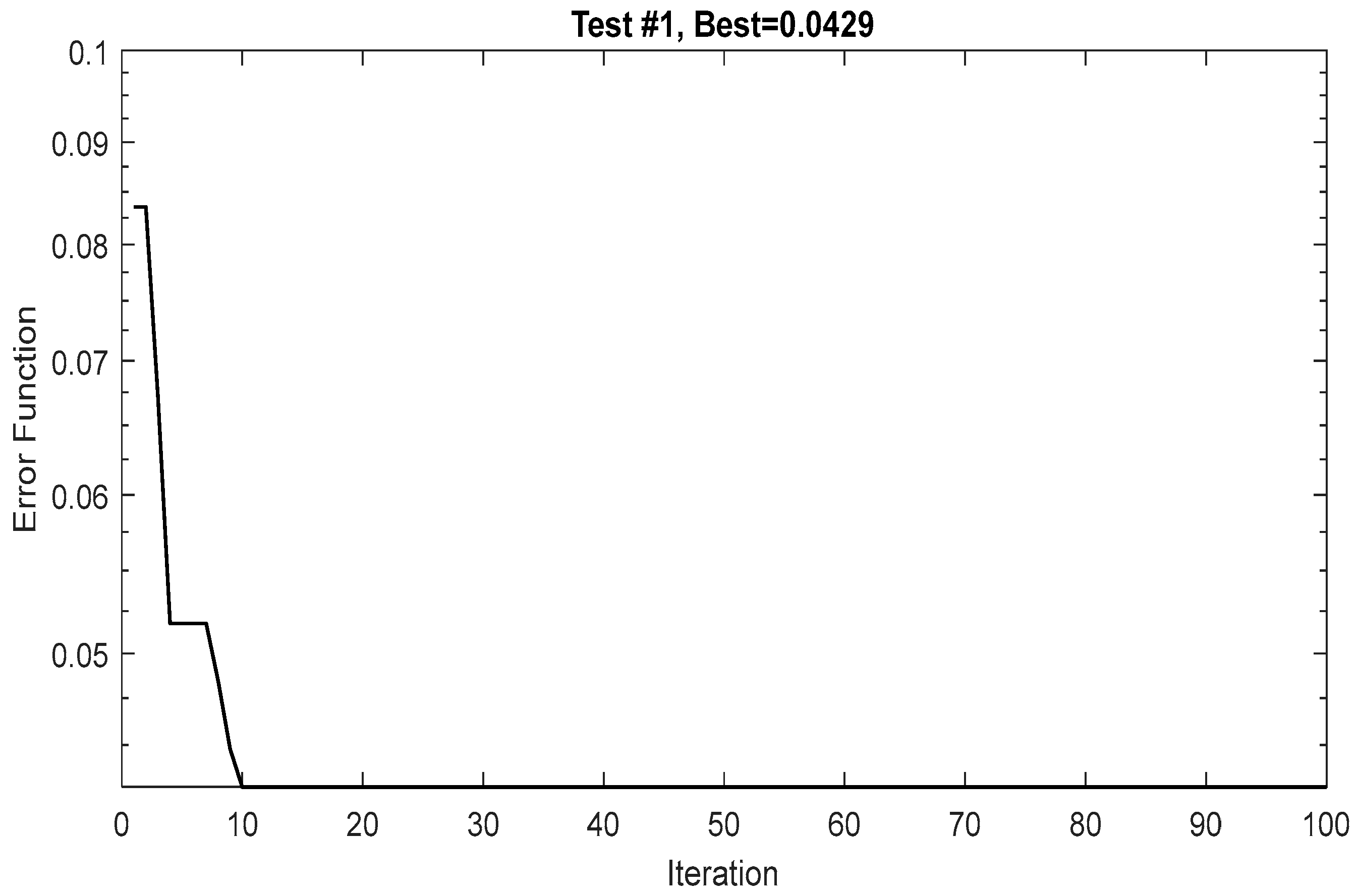
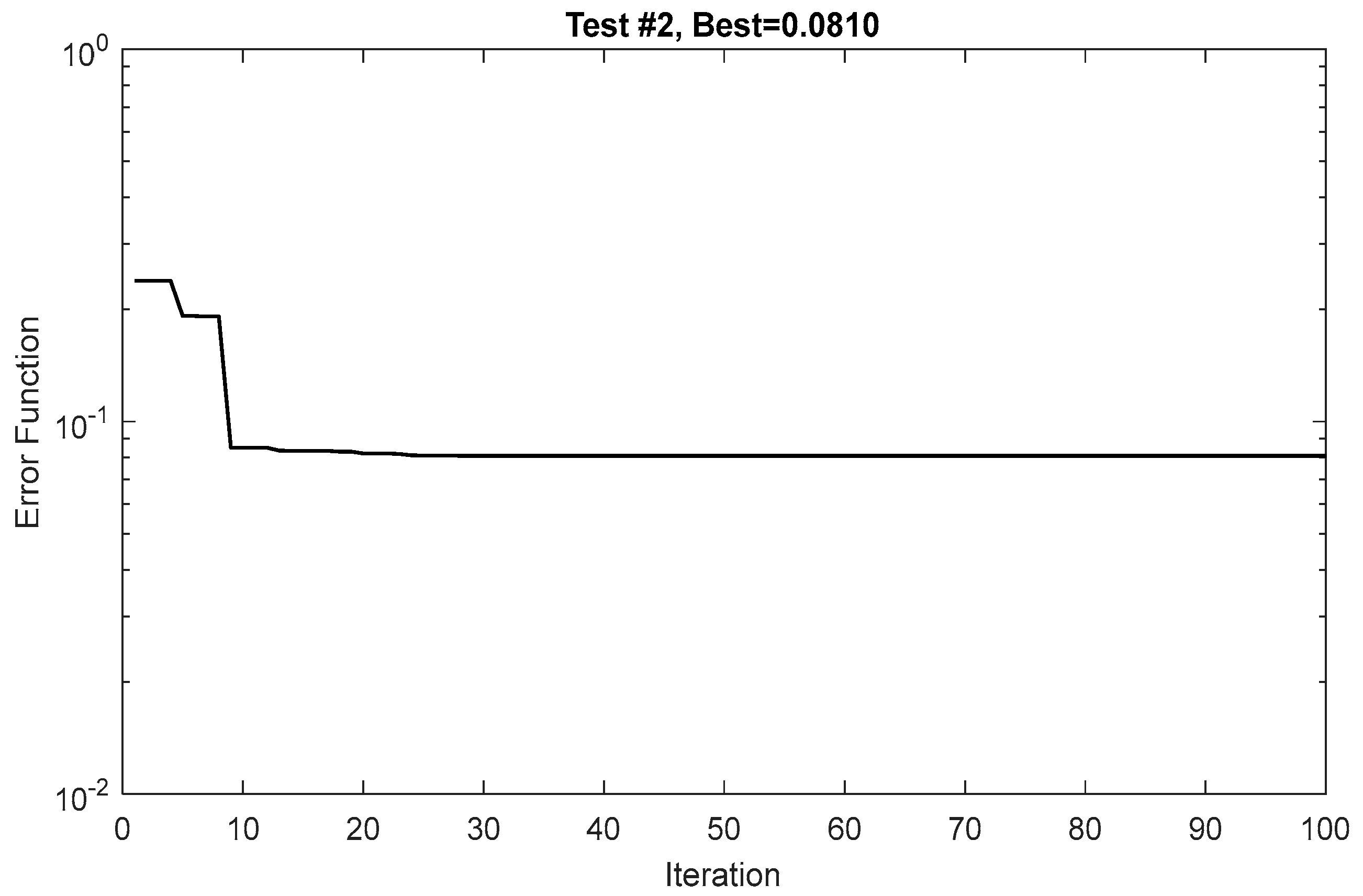
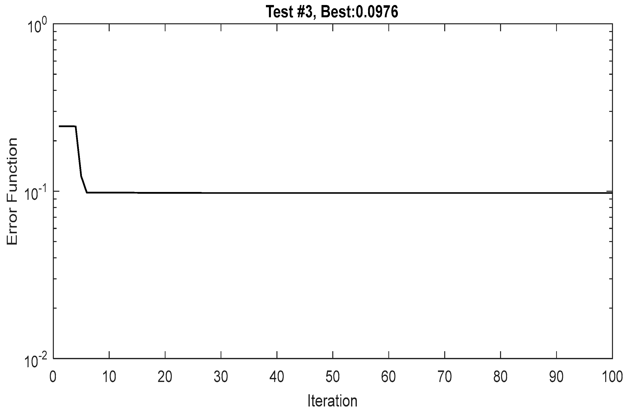
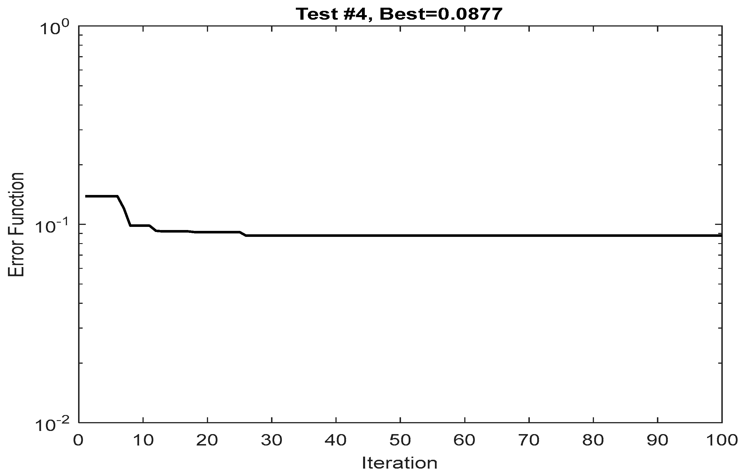
2.3. Problem Solving and Objective Function

As mentioned in the previous sections, the proposed model includes two tuning parameters (exponential function coefficient n and the transition region thickness $\delta$), which are altered with the aid of Genetic Algorithm (GA) to minimize the error between calculated oil productions obtained from the developed equations (Equations (23), (24), (46), and (47)) and the experimentally measured data. For such purposes, the error function provided in Equation (49) is used in this study:

$$E\left(n,\delta \right)=E\left(n,\delta \right)=\frac{{\sum }_{i=1}^{Nt}\frac{\left|Q_{m, t_i}-Q_{c, t_i}\right|}{Q_{m, t_i}}}{Nt}$$

(49)

where, $Q_{m, i}$ is the measured cumulative produced oil at $t=t_i$, $Q_{c, i}$ is the theoretical cumulative produced oil using the exponential solvent chamber model at $t=t_i$, and $Nt$ is the total number of measured data by the end of the process.

3. Results and Discussion

The proposed model was analyzed by applying it to the four VAPEX cases presented by Ma et al. [3].

Table 1. Heavy oil and physical model properties for the experimental cases presented by Ma et al. [3].

Test No.	$\mathit{\varphi }$ (%)	$\mathit{k}$$\left(\mathsf{\mu }{\mathbf{m}}^2\right)$	${\mathit{\rho }}_{\mathit{o}}\left({\mathit{C}}_{\mathit{m}\mathit{a}\mathit{x}}\right)$$\left(\frac{\mathbf{g}}{\mathbf{c}\mathbf{c}}\right)$	${\mathit{\mu }}_{\mathit{o}}\left({\mathit{C}}_{\mathit{m}\mathit{a}\mathit{x}}\right) \left(\mathbf{m}\mathbf{P}\mathbf{a}.\mathbf{s}\right)$	H (cm)	W (cm)	d (cm)	${\mathit{S}}_{\mathit{o}}$	${\mathit{S}}_{\mathit{o}\mathit{r}}$
1	31.4	152	0.828	8.51	10	20	2	0.975	0.085
2	32.9	52	0.828	8.51	10	20	2	0.977	0.071
3	35.7	18	0.828	8.51	10	20	2	0.962	0.109
4	36.3	8	0.828	8.51	10	20	2	0.962	0.106

summarizes the heavy oil and the physical model properties used in their experiments. Furthermore, Figure 9, Figure 10 and Figure 11 illustrate cumulative produced oil, the heavy oil production rate, and the transition region thickness for the experimental cases reported by Ma et al. [3], respectively.

To find the optimized values of $\delta$ and n, the objective function in Equation (45) was minimized using a MATLAB-based Genetic Algorithm (GA) [20] in the above-mentioned experimental cases.

Table 2. The determined values of the unknown parameters.

Test No.	Solvent Chamber Shape	n	$\mathit{\delta }$ (cm)
1	Concave	0.1343	0.2567
2	Concave	0.0459	0.1905
3	Convex	0.0919	0.3867
4	Convex	0.0322	0.3972

reveals those values. Moreover, Figure 12, Figure 13, Figure 14 and Figure 15 visualize the discrepancies in the error function at each iteration of the GA, for the first four tests, respectively.

Furthermore, the minimum values obtained for the error function at each test are provided in

Table 3. Best values of error function at each test.

Test No.	Minimum Value of Error Function
Test #1	0.0429
Test #2	0.0810
Test #3	0.0976
Test #4	0.0877

.

In addition, to further investigate the overall performance of the model, the following sections compare the determined solvent chamber propagation at different stages, transition region thicknesses, and values of cumulative produced oil, along with the oil production rate, to those measured by Ma et al. [3].

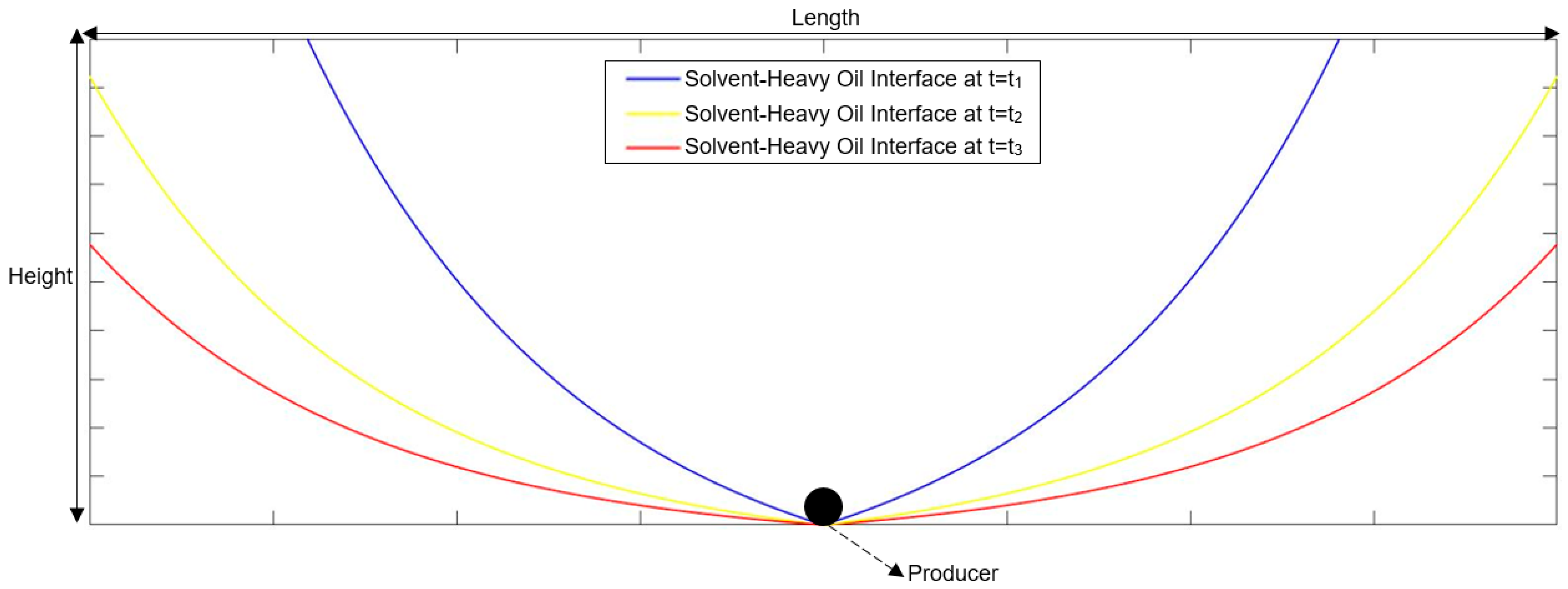
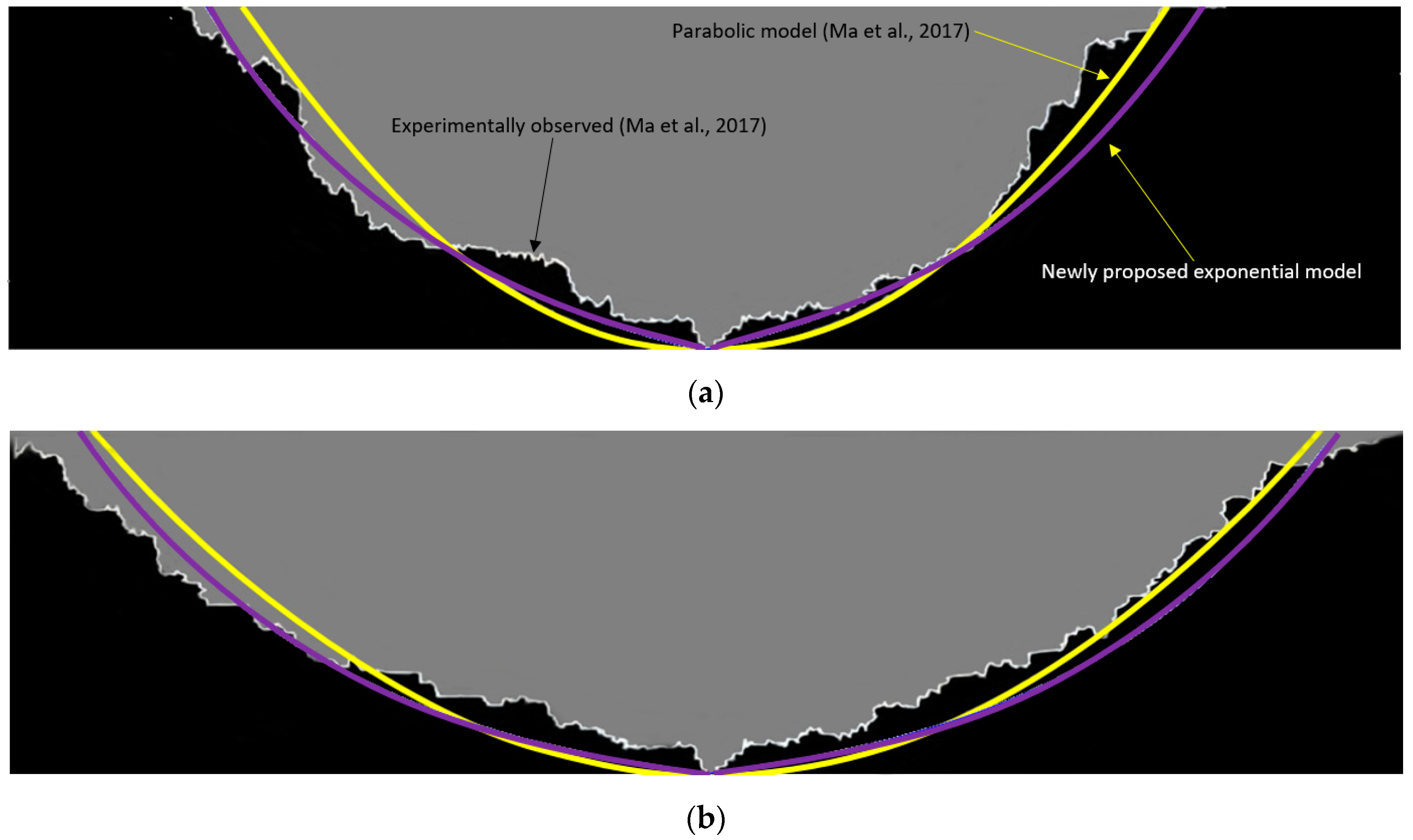
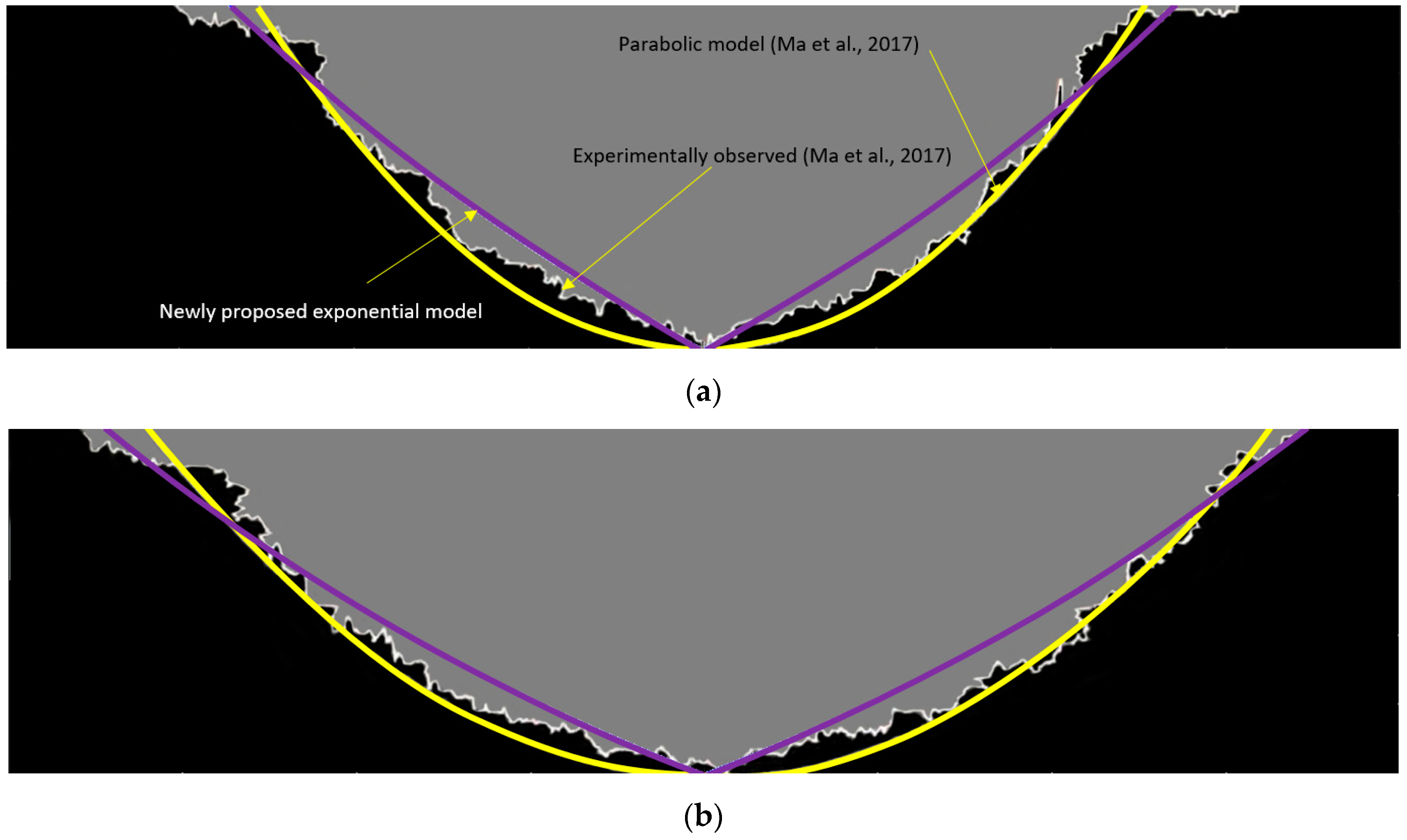
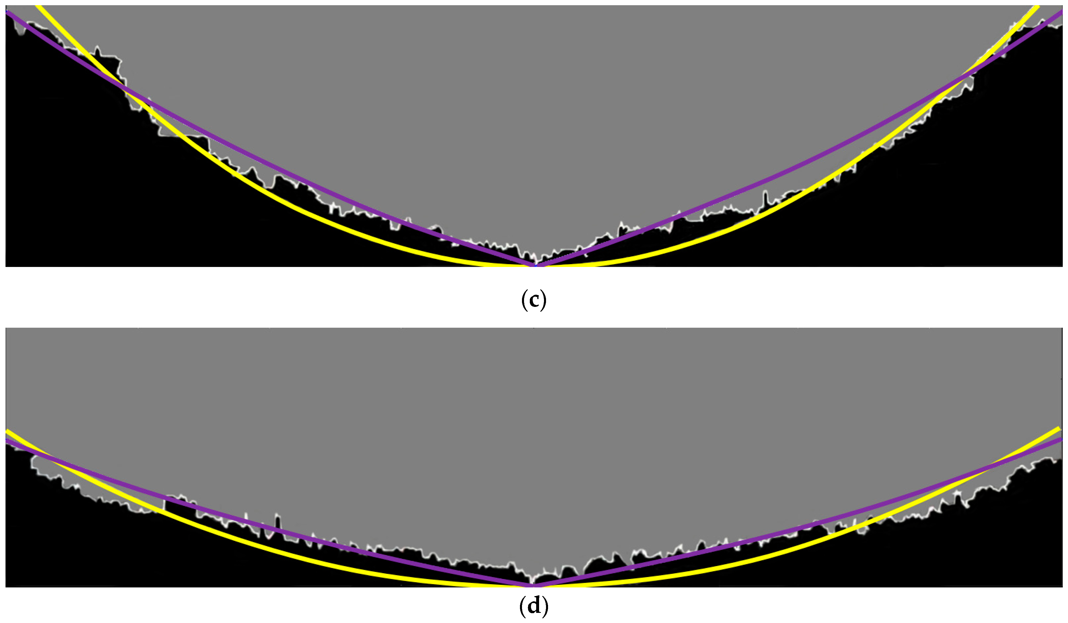
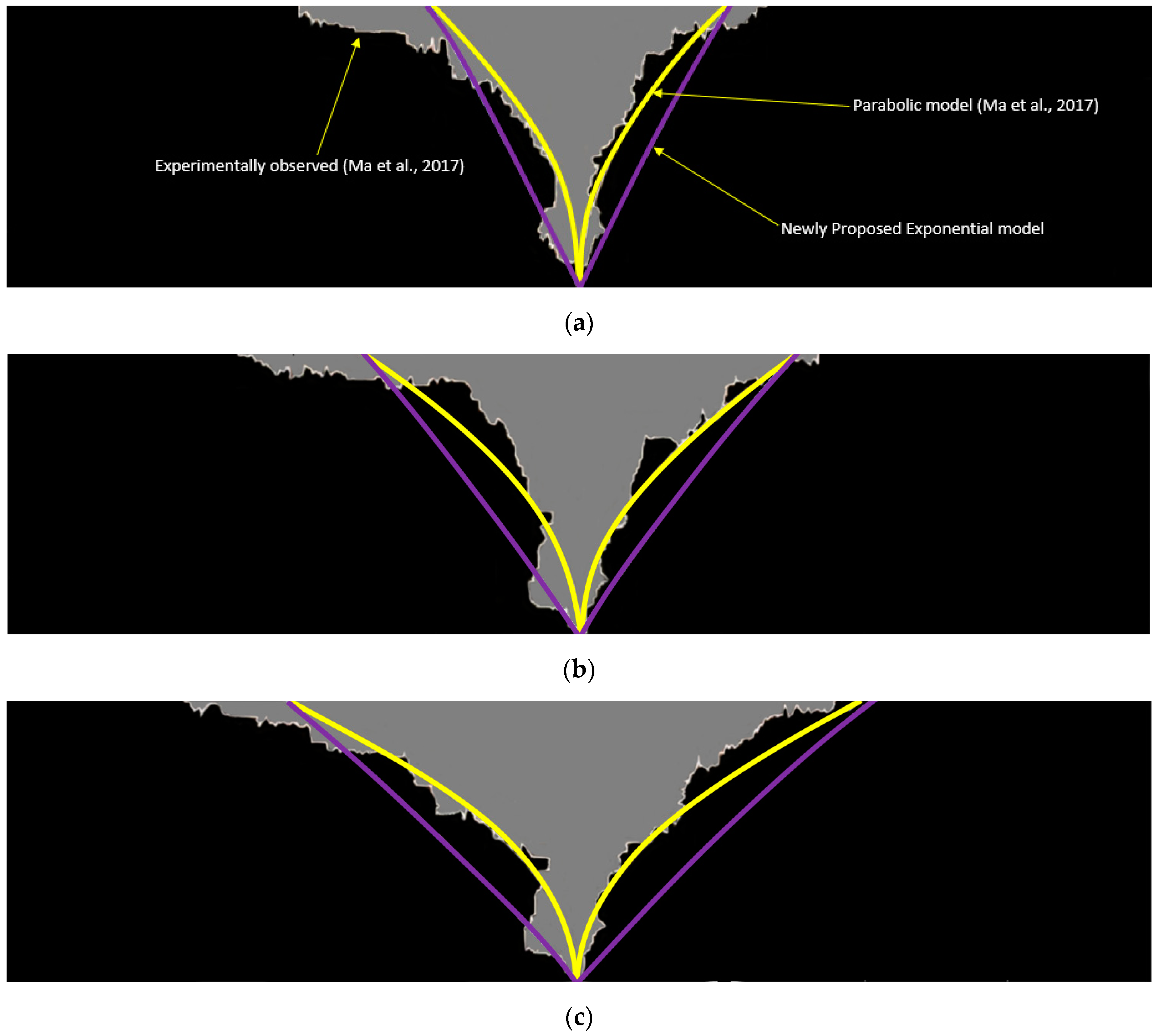
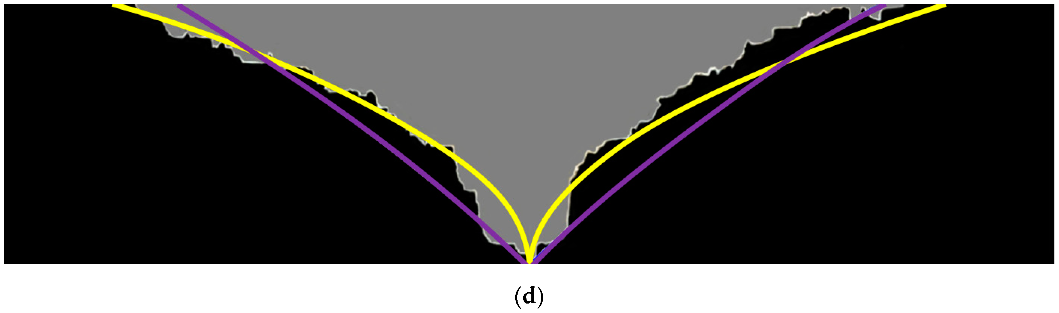
3.1. Solvent Chamber Propagation

In this section, a comparison is conducted between the solvent chambers generated by the newly proposed exponential model, those observed experimentally by Ma et al. [3], and the solvent chambers calculated by their parabolic model in order to assess the accuracy of the proposed model in predicting solvent chamber propagation. Results show that the newly proposed exponential model is capable of accurately predicting the solvent chamber propagation at both the spreading and falling stages. Figure 16, Figure 17, Figure 18 and Figure 19 illustrate the comparison of the newly proposed exponential model, the parabolic model, and the experimentally measured solvent chambers for the first four tests, respectively.

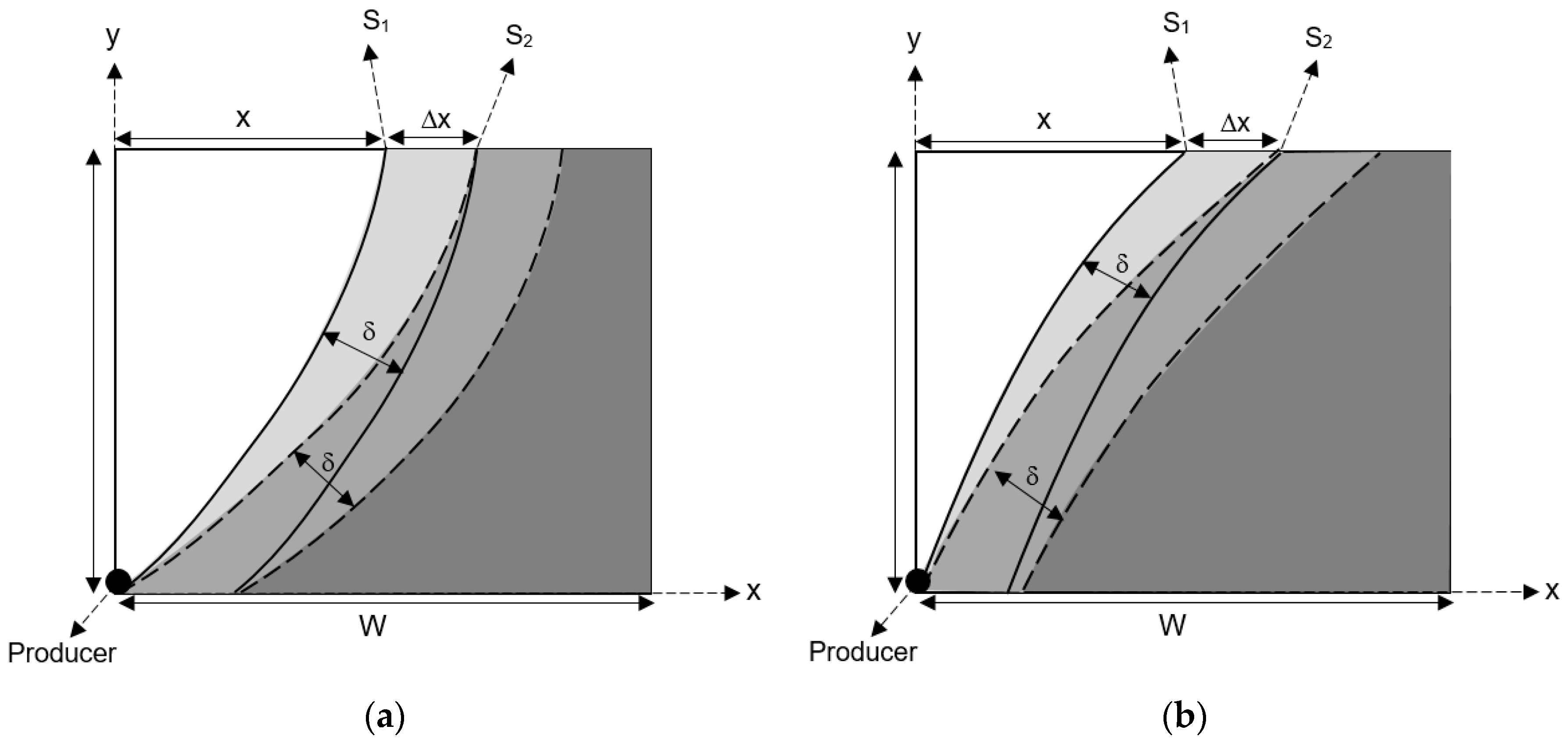
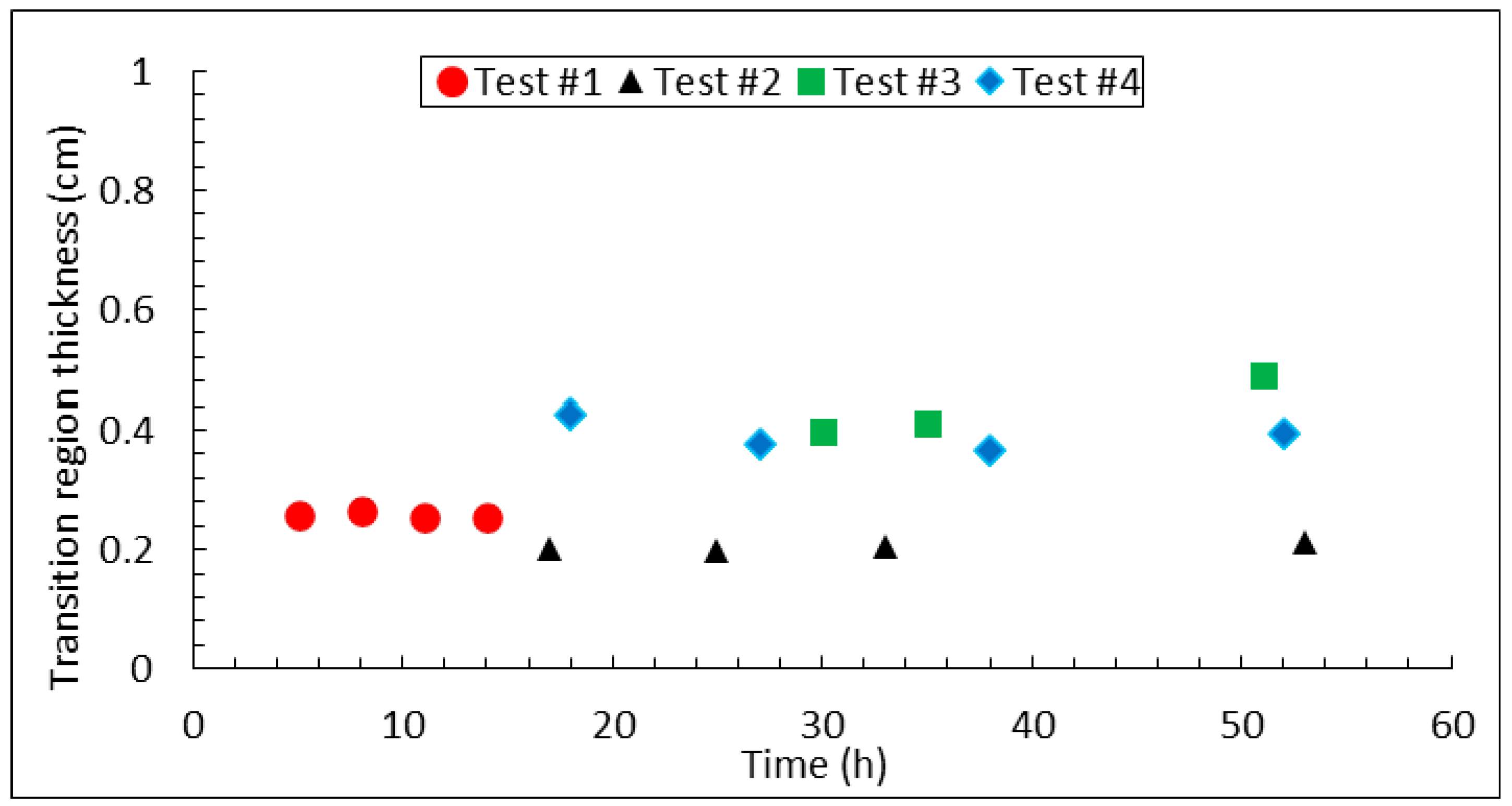
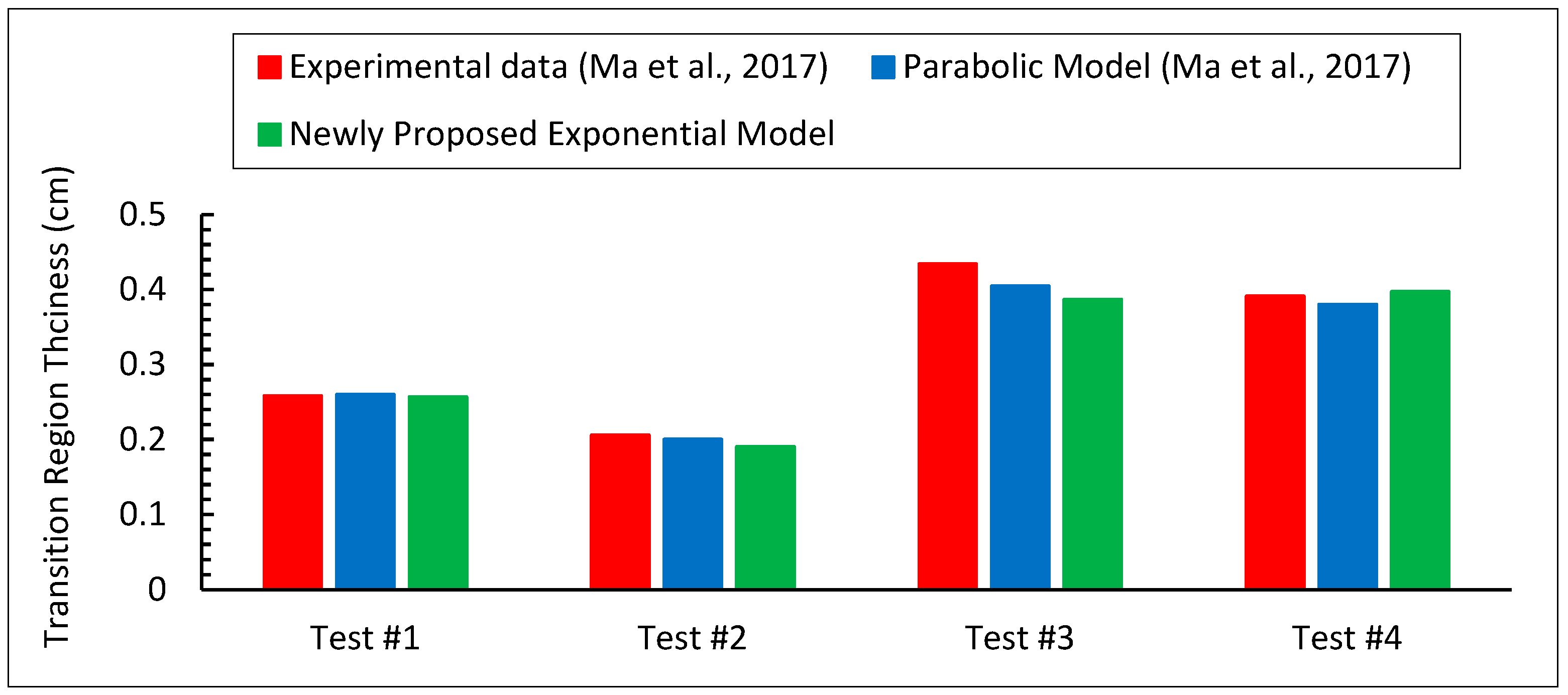
3.2. Transition Region Thickness

The thickness of the transition regions determined by the proposed model and those calculated and measured by Ma et al. [3] are shown in Figure 20. Based on the figure, it is evident that the transition region thickness determined by the proposed method closely matches the transition region thicknesses determined in the laboratory, and the average relative error of all cases for this parameter was found to be 5.12%.

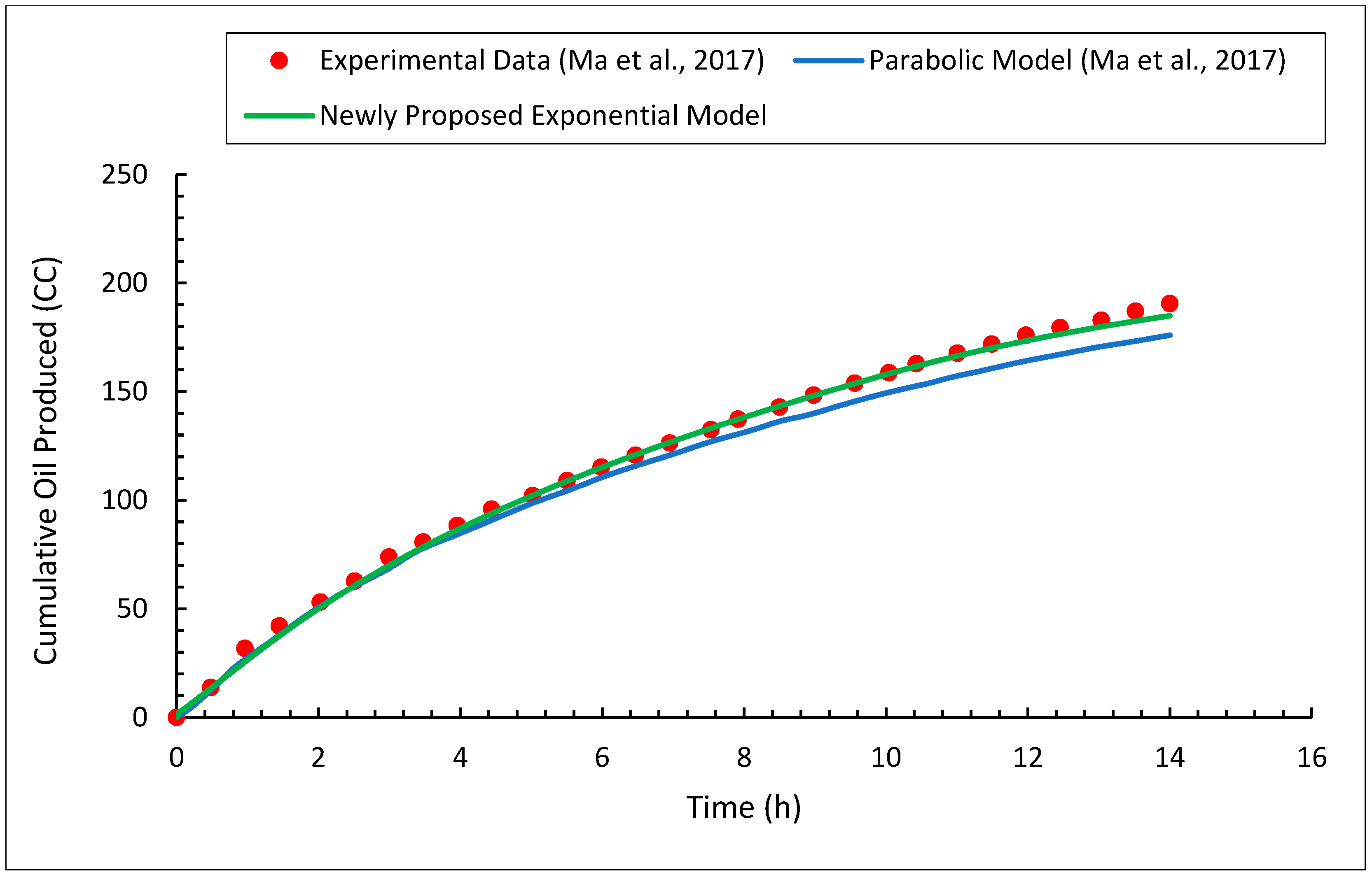
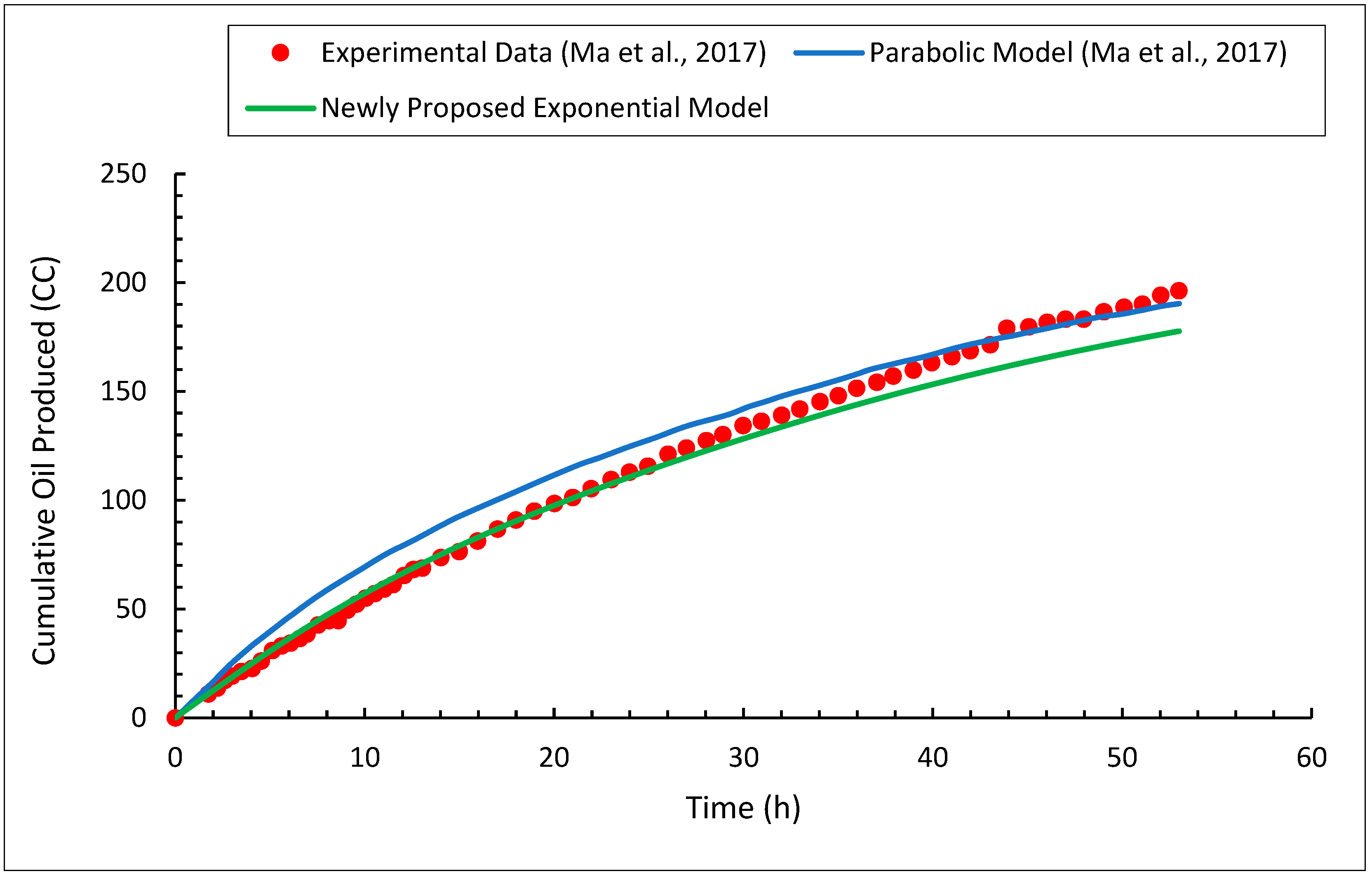
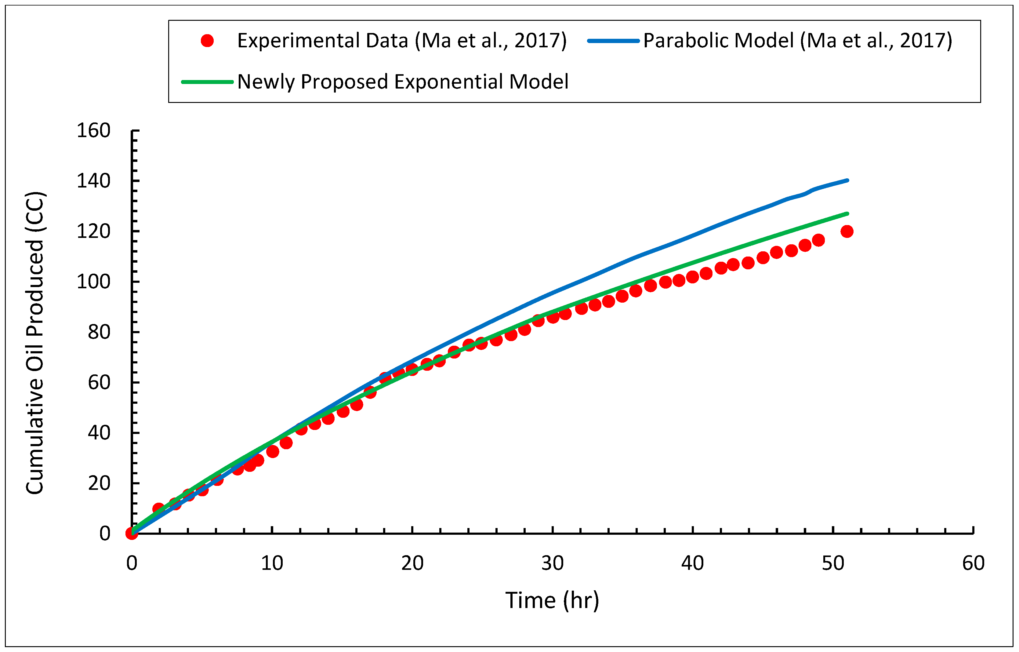
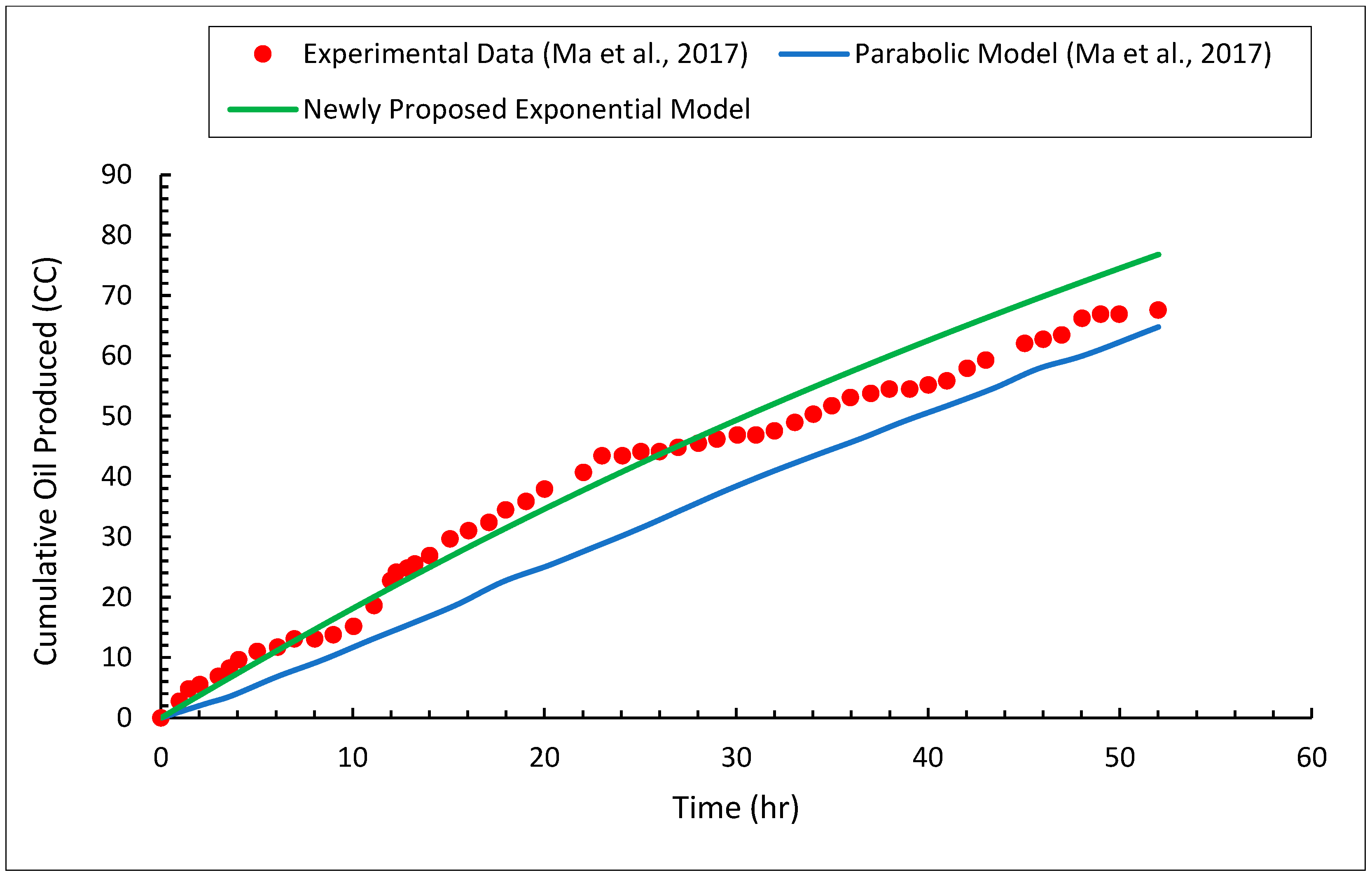
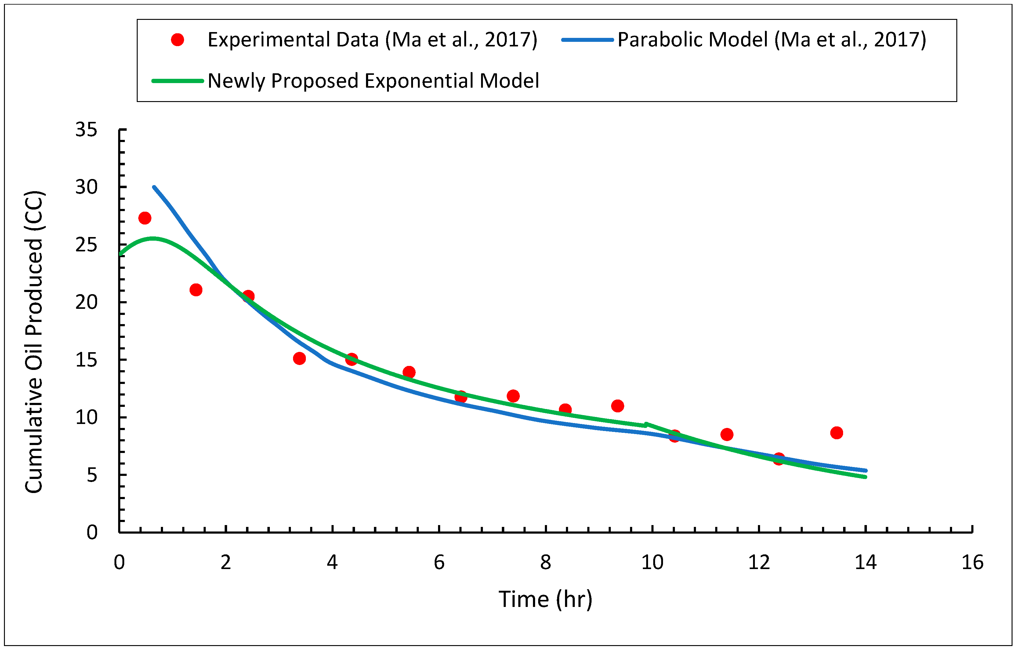
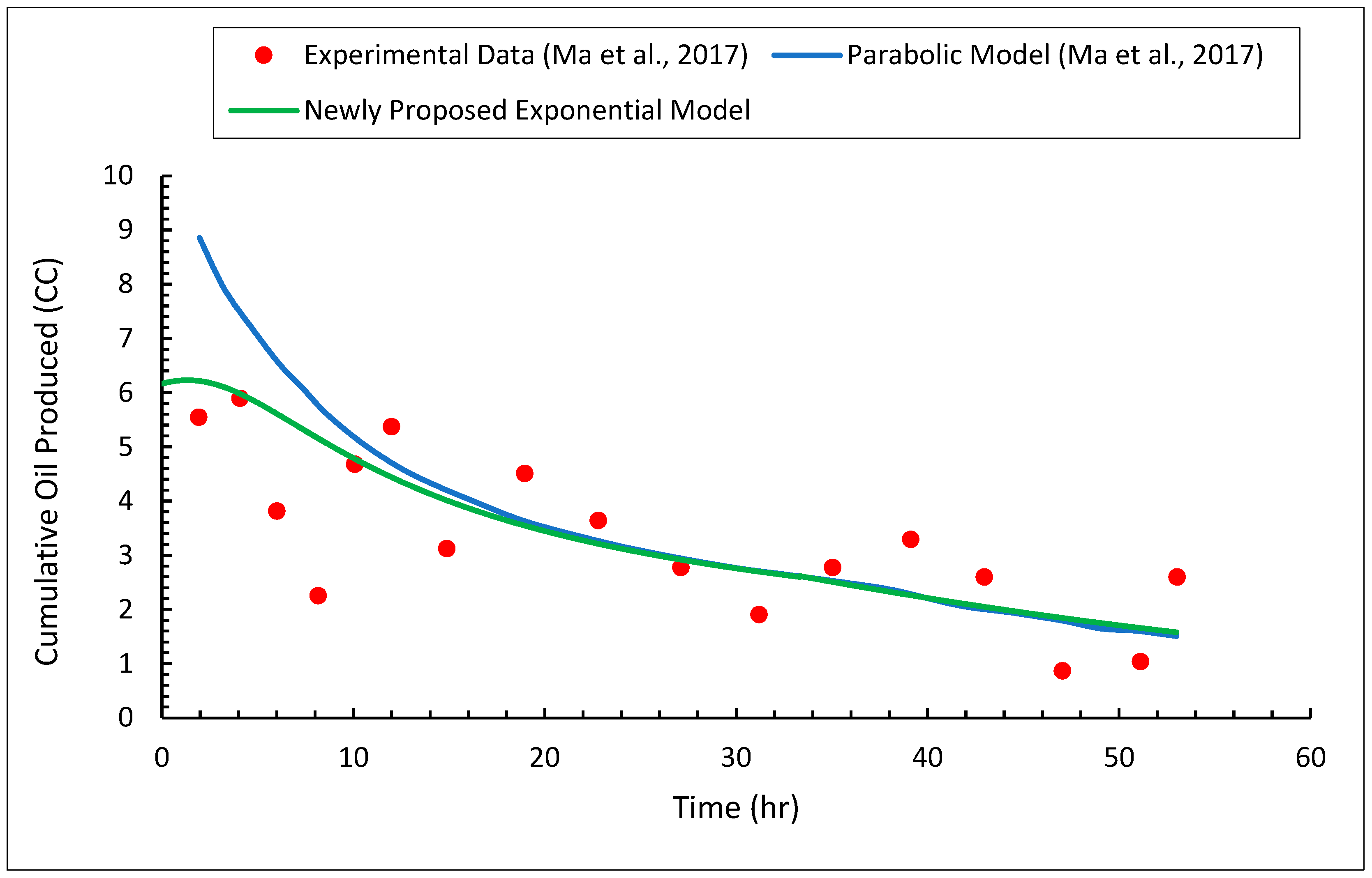
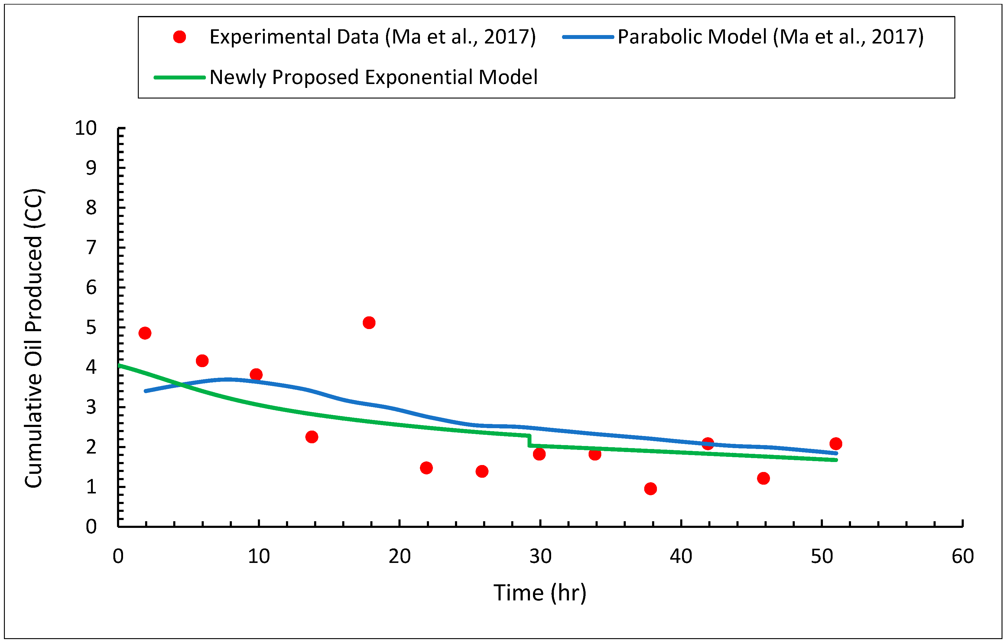
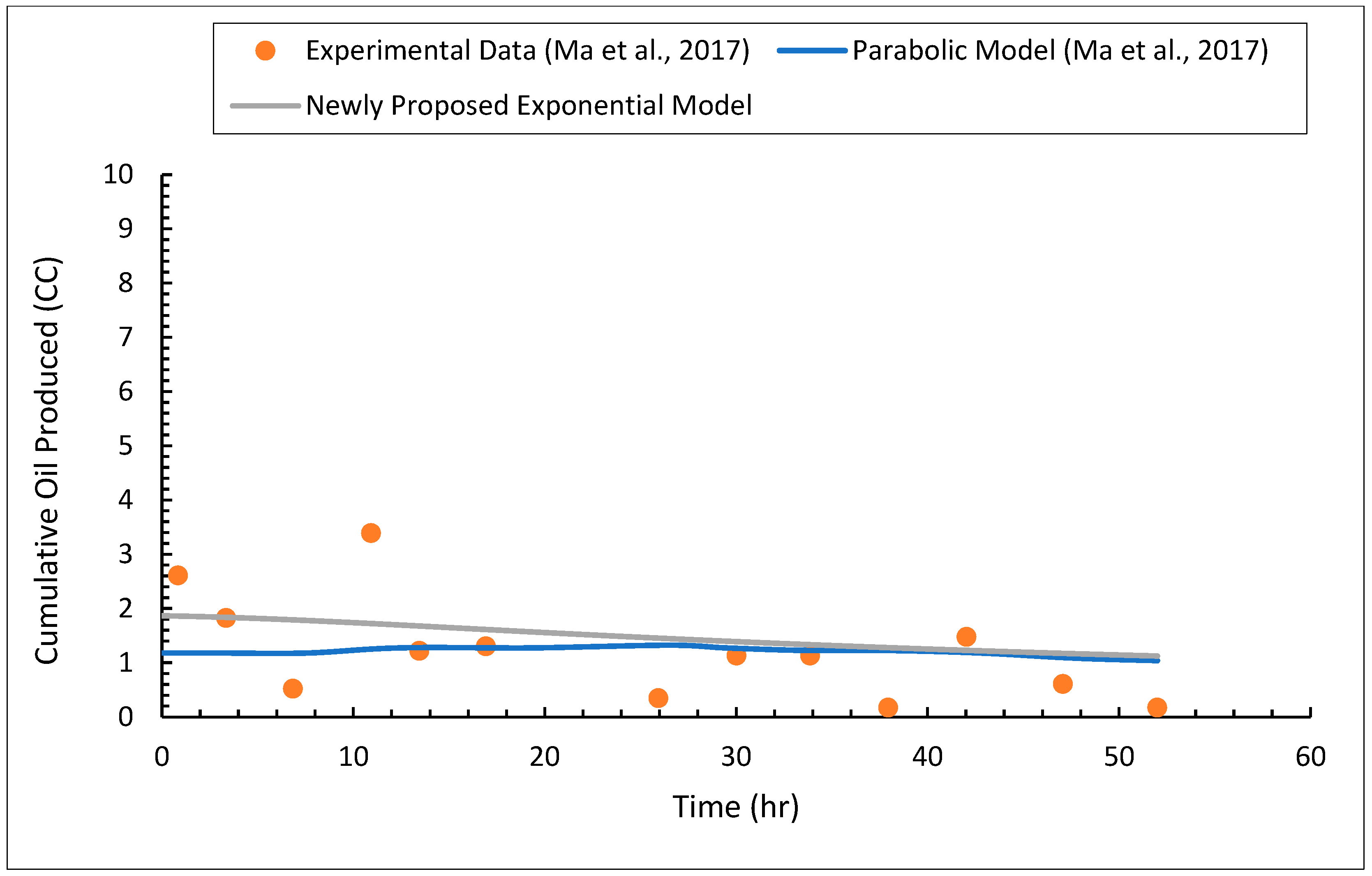
3.3. Heavy Oil Production

Finally, the proposed model was employed to determine both the cumulative produced oil and the heavy oil production rate. As shown in Figure 21, Figure 22, Figure 23 and Figure 24, cumulative produced oil from the newly proposed exponential model was juxtaposed with experimental data and the cumulative produced oil from the parabolic model proposed by Ma et al. [3]. As can be seen, the cumulative heavy oil production data estimated by the exponential model agree well with the experimental results reported by Ma et al. [3], with the average relative errors of all four cases for this parameter being between 7 and 8%. Additionally, the proposed model is more accurate with regard to heavy oil production when compared with the Ma et al. model [3], as they reported an average relative error of 14.8% for this parameter. In addition, Figure 25, Figure 26, Figure 27 and Figure 28 show the oil production rate estimated by the newly proposed exponential model, the experimental data, and the oil production rate estimated by the parabolic model proposed by Ma et al. Accordingly, the anticipated oil production rates are in acceptable agreement with the experimental findings.

4. Conclusions

In this study, the spreading and falling stages of the solvent chamber were modeled using an exponential solvent chamber geometry. In this newly proposed model, the total produced oil at both the spreading and falling stages can be accurately adjusted to the measured values. A reasonable agreement was found between the thickness of the transition region obtained by this model and the existing experimental measurements. As a result, the suggested model is capable of accurately anticipating the heavy oil production rate, and the evaluated solvent chamber shapes match well with those observed in the four experimental cases used in this study for validation. The proposed model was also compared to the parabolic model developed by Ma et al. [3]. The results reveal that the newly proposed exponential model outperforms the parabolic model in terms of heavy oil production estimation. Exponential model’s average relative error of 7.73% for the cumulative oil production in all four experimental cases is more accurate than the parabolic model value of 14.8%. It is also important to note that the performance of the newly proposed model needs to be further analyzed by applying it to more complex conditions. Sensitivity analysis should be conducted on the influencing parameters, such as the solvent type, the heterogeneity of the porous media, and the physical model dimensions. Furthermore, the application of the proposed model at a larger scale needs to be further investigated. The five major findings of this study are as follows:

• Using the proposed exponential model, the solvent chamber, heavy oil production rate, and cumulative heavy oil production can be accurately predicted.
• With a relative error of less than 5.12%, the newly proposed model closely matches the measurements of transition region thickness.
• The exponential model can accurately predict the transition region thicknesses, with the average relative errors of all cases being around 7.73%.
• The assumption of constant transition region thickness reduces the complexity of the model and produces reliable results.
• It seems reasonable to ignore the rising stage due to its insignificant impacts on the overall performance of the model, which confirms the findings in the literature [3,14].

References

1. Butler, R.M.; Mokrys, I.J. A new process (VAPEX) for recovering heavy oils using hot water and hydrocarbon vapour. J. Can. Pet. Technol. 1991, 30, PETSOC-91-01-09. [Google Scholar] [CrossRef]
2. Das, S.K.; Butler, R.M. Mechanism of the vapor extraction process for heavy oil and bitumen. J. Pet. Sci. Eng. 1998, 21, 43–59. [Google Scholar] [CrossRef]
3. Ma, H.; Yu, G.; She, Y.; Gu, Y. A parabolic solvent chamber model for simulating the solvent vapor extraction (VAPEX) heavy oil recovery process. J. Pet. Sci. Eng. 2017, 149, 465–475. [Google Scholar] [CrossRef]
4. Karmaker, K.; Maini, B.B. Applicability of vapor extraction process to problematic viscous oil reservoirs. In Proceedings of the SPE Annual Technical Conference and Exhibition, Denver, CO, USA, 5–8 October 2003; OnePetro: Richardson, TX, USA, 2003. [Google Scholar]
5. Singhal, A.; Das, S.; Leggitt, S.; Kasraie, M.; Ito, Y. Screening of reservoirs for exploitation by application of steam assisted gravity drainage/vapex processes. In Proceedings of the International Conference on Horizontal Well Technology, Calgary, AB, Canada, 18–20 November 1996; OnePetro: Richardson, TX, USA, 1996. [Google Scholar]
6. Luo, P.; Gu, Y. Effects of asphaltene content and solvent concentration on heavy oil viscosity. In Proceedings of the SPE International Thermal Operations and Heavy Oil Symposium, Calgary, AB, Canada, 1–3 November 2005; OnePetro: Richardson, TX, USA, 2005. [Google Scholar]
7. Qi, R. Simulation Study of Warm VAPEX Process Using Water-Soluble Solvent. Master’s Thesis, Schulich School of Engineering, Calgary, AB, Canada, 2020. [Google Scholar]
8. Xu, J.; Chen, Z.; Dong, X.; Zhou, W. Effects of lean zones on steam-assisted gravity drainage performance. Energies 2017, 10, 471. [Google Scholar] [CrossRef]
9. Xu, J.; Chen, Z.; Cao, J.; Li, R. Numerical study of the effects of lean zones on SAGD performance in periodically heterogeneous media. In Proceedings of the SPE Heavy Oil Conference-Canada, Calgary, AB, Canada, 10–12 June 2014; OnePetro: Richardson, TX, USA, 2014. [Google Scholar]
10. Butler, R.; Mokrys, I. Solvent Analog Model of Steam-Assisted Gravity Drainage. AOSTRA J. Res. 1989, 5, 17, (Reprint). [Google Scholar]
11. Yazdani, A.; Maini, B.B. Modeling of the VAPEX process in a very large physical model. Energy Fuels 2008, 22, 535–544. [Google Scholar] [CrossRef]
12. Wang, Q.; Jia, X.; Chen, Z. Mathematical modeling of the solvent chamber evolution in a vapor extraction heavy oil recovery process. Fuel 2016, 186, 339–349. [Google Scholar] [CrossRef]
13. Moghadam, S.; Nobakht, M.; Gu, Y. Theoretical and physical modeling of a solvent vapour extraction (VAPEX) process for heavy oil recovery. J. Pet. Sci. Eng. 2009, 65, 93–104. [Google Scholar] [CrossRef]
14. Lin, L.; Zeng, F.; Gu, Y. A circular solvent chamber model for simulating the VAPEX heavy oil recovery process. J. Pet. Sci. Eng. 2014, 118, 27–39. [Google Scholar] [CrossRef]
15. Cuthiell, D.; McCarthy, C.; Frauenfeld, T.; Cameron, S.; Kissel, G. Investigation of the VAPEX process using CT scanning and numerical simulation. J. Can. Pet. Technol. 2003, 42, PETSOC-03-02-04. [Google Scholar] [CrossRef]
16. Nghiem, L.; Kohse, B.; Sammon, P. Compositional simulation of the VAPEX process. J. Can. Pet. Technol. 2001, 40, PETSOC-01-08-05. [Google Scholar] [CrossRef]
17. Nourozieh, H.; Kariznovi, M.; Abedi, J.; Chen, Z.J. A new approach to simulate the boundary layer in the vapour extraction process. J. Can. Pet. Technol. 2011, 50, 11–18. [Google Scholar] [CrossRef]
18. Yazdani, A.; Maini, B.B. Pitfalls and solutions in numerical simulation of VAPEX experiments. Energy Fuels 2009, 23, 3981–3988. [Google Scholar] [CrossRef]
19. Chapra, S.C. Applied Numerical Methods with MATLAB for Engineers and Scientists; McGraw-Hill Higher Education: New York, NY, USA, 2008. [Google Scholar]
20. McCall, J. Genetic algorithms for modelling and optimisation. J. Comput. Appl. Math. 2005, 184, 205–222. [Google Scholar] [CrossRef]
Figure 1. Concave exponential propagation of solvent chamber throughout the spreading and falling stages.
Energies 15 05874 g001
Figure 2. Convex exponential propagation of solvent chamber throughout the spreading and falling stages.
Energies 15 05874 g002
Figure 3. The diluted heavy oil velocity within the transition region of (a) concave case and (b) convex case.
Energies 15 05874 g003
Figure 4. The transition region propagation at the spreading phase having a (a) concave shape and (b) convex shape.
Energies 15 05874 g004
Figure 5. Solvent chamber area for one side of the physical model in the (a) concave case and (b) convex case.
Energies 15 05874 g005
Figure 6. Falling stage of one side of the physical model in the (a) concave case and (b) convex case.
Energies 15 05874 g006
Figure 7. Axial falling of the chamber during the falling stage of the (a) concave case and (b) convex case.
Energies 15 05874 g007
Figure 8. Solvent chamber area for one side of the physical model at the falling stage of the (a) concave case and (b) convex case.
Energies 15 05874 g008
Figure 9. Actual cumulative production data for the experimental cases presented by Ma et al. [3].
Energies 15 05874 g009
Figure 10. Actual oil production rate data for the experimental cases presented by Ma et al. [3].
Energies 15 05874 g010
Figure 11. Actual transition region thickness values for the experimental cases presented by Ma et al. [3].
Energies 15 05874 g011
Figure 12. Variation in the error function at each iteration of the Genetic Algorithm in test #1.
Energies 15 05874 g012
Figure 13. Variation in the error function at each iteration of the Genetic Algorithm in test #2.
Energies 15 05874 g013
Figure 14. Variation in the error function at each iteration of the Genetic Algorithm in test #3.
Energies 15 05874 g014
Figure 15. Variation in the error function at each iteration of the Genetic Algorithm in test #4.
Energies 15 05874 g015
Figure 16. Comparison of the solvent chambers estimated by exponential model, solvent chambers estimated by parabolic model [3], and experimentally visualized [3] solvent chambers in test #1 at (a) t = 5 h, (b) t = 8 h, (c) t = 11 h, and (d) t = 14 h.
Energies 15 05874 g016aEnergies 15 05874 g016b
Figure 17. Comparison of the solvent chambers estimated by exponential model, solvent chambers estimated by parabolic model [3], and experimentally visualized [3] solvent chambers in test #2 at (a) t = 17 h, (b) t = 25 h, (c) t = 33 h, and (d) t = 53 h.
Energies 15 05874 g017aEnergies 15 05874 g017b
Figure 18. Comparison of the solvent chambers estimated by exponential model, solvent chambers estimated by parabolic model [3], and experimentally visualized [3] solvent chambers in test #3 at (a) t = 30 h, (b) t = 35 h, (c) t = 51 h.
Energies 15 05874 g018aEnergies 15 05874 g018b
Figure 19. Comparison of the solvent chambers estimated by exponential model, solvent chambers estimated by parabolic model [3], and experimentally visualized [3] solvent chambers in test #4 at (a) t = 18 h, (b) t = 27 h, (c) t = 38 h, and (d) t = 52 h.
Energies 15 05874 g019aEnergies 15 05874 g019b
Figure 20. Comparison of the average transition region thickness values [3].
Energies 15 05874 g020
Figure 21. Comparison of the cumulative produced oil estimated by the newly proposed exponential model, experimentally measured cumulative produced oil [3], and cumulative produced oil estimated by the parabolic model proposed by Ma et al. [3] in test #1.
Energies 15 05874 g021
Figure 22. Comparison of the cumulative produced oil estimated by the newly proposed exponential model, experimentally measured cumulative produced oil [3], and cumulative produced oil estimated by the parabolic model proposed by Ma et al. [3] in test #2.
Energies 15 05874 g022
Figure 23. Comparison of the cumulative produced oil estimated by the newly proposed exponential model, experimentally measured cumulative produced oil [3], and cumulative produced oil estimated by the parabolic model proposed by Ma et al. [3] in test #3.
Energies 15 05874 g023
Figure 24. Comparison of the cumulative produced oil estimated by the newly proposed exponential model, experimentally measured cumulative produced oil [3], and cumulative produced oil estimated by the parabolic model proposed by Ma et al. [3] in test #4.
Energies 15 05874 g024
Figure 25. Comparison of the oil production rate estimated by the newly proposed exponential model, experimentally measured oil production rate [3], and oil production rate estimated by the parabolic model proposed by Ma et al. [3] in test #1.
Energies 15 05874 g025
Figure 26. Comparison of the oil production rate estimated by the newly proposed exponential model, experimentally measured oil production rate [3], and oil production rate estimated by the parabolic model proposed by Ma et al. [3] in test #2.
Energies 15 05874 g026
Figure 27. Comparison of the oil production rate estimated by the newly proposed exponential model, experimentally measured oil production rate [3], and oil production rate estimated by the parabolic model proposed by Ma et al. [3] in test #3.
Energies 15 05874 g027
Figure 28. Comparison of the oil production rate estimated by the newly proposed exponential model, experimentally measured oil production rate [3], and oil production rate estimated by the parabolic model proposed by Ma et al. [3] in test #4.
Energies 15 05874 g028