Pressure Drop Prediction of Crude Oil Pipeline Based on PSO-BP Neural Network

Abstract

Pipeline transportation of crude oil has great advantages over traditional oil transmission methods, in terms of economic and environmental protection. The main costs in the oilfield surface system are the fuel costs for heating the crude oil during transportation and the electricity costs for the pumping units. In the northeast of China, where winter temperatures are extremely low and the oil has a high freezing point and high viscosity, higher temperatures, and pressures are required to transport crude oil. With machine learning widely used in many industries and achieving better results, the digital management of oil pipelines has stored a large amount of production and operation data, which has laid the foundation for the research of oil pipeline process calculation using machine learning methods. In this paper, a crude oil pressure drop calculation of an oil pipeline in Northeast China is carried out based on a neural network. For pipeline pressure drop calculation, the back propagation neural network (BP) pressure drop calculation model and particle swarm optimization for back propagation neuron network (PSO-BP) pressure drop calculation model are established. Two models were used to calculate and compare the measured data, and the average absolute error of the PSO-BP model was the smallest, which was 0.015%. Compared with the BP model, the average relative error is reduced by 13.16%. Therefore, The PSO-BP pressure drop calculation model has high accuracy and is of practical significance for predicting pipeline pressure drop.

1. Introduction

The winter temperatures in northeast China are extremely low, and the difference between the transport temperature of oil and the soil temperature is significant. The pipeline dissipates heat faster, the oil cools down faster, and the hydraulic friction coefficient then increases, which also has an impact on the pressure change of the pipeline. In the field of oil pipeline, support vector machines (SVM), the BP neural network has good performance in the prediction of pipeline energy consumption, pipeline corrosion detection, pipeline temperature calculation, and so on. Chinese scholars have thoroughly researched its application to pipelines and calculated and verified it combined with the actual data [1]. From the results of previous studies, it is found that SVM is generally used for machine learning problems under small samples. It is poorly trained for large-scale datasets, as there is no general solution for nonlinear problems, and it is difficult to find a suitable kernel function. Due to a large number of data sets in this study and the nonlinear correlation of the data, BP neural network is more suitable. Yuan Guo predicted small leaks in hydraulic cylinders, applying a convolutional neural network, BP neural network, T-S neural network, and Elman neural network, and the accuracy of the prediction results were above 90% [2]. Han Wei adopted the performance prediction method of a centrifugal pump based on the LM training algorithm and double hidden layer BP neural network. The average relative error between the model prediction efficiency and the experimental efficiency is 2.94% [3]. Tiezhu Sun developed a BP neural network prediction model based on a particle swarm algorithm and predicted the performance of a dew point indirect evaporative cooler. By comparing the prediction results with the traditional BP neural network, the author showed that the PSO-BP model has higher accuracy [4]. Li Shubin used a neural network to build a pipeline prediction model instead of a traditional pipeline mathematical model to calculate pressure [5]. Gao Shanbu, Qian Chengwen, and others joined the error control formula to the traditional BP neural network prediction process, and finally established, based on an improved BP neural network, a crude oil pipeline energy consumption prediction model [6]. Hou Lei et al. accurately calculated the energy consumed in the operation of the oil pipeline. By analyzing the operation report of the oil pipeline, the main energy consumption indexes in the evaluation of the oil production process were determined, and the BP neural network was used to establish the energy consumption prediction model of the oil pipeline [7]. Using the pressure gradient method, Junhua Li et al. found that the accuracy of locating the pipeline leak point is greatly affected by the friction coefficient, and the traditional method of determining the friction coefficient does not apply to the actual operating leaky pipeline. As a result, they proposed a leak point location method based on the BP neural network prediction of the friction coefficient, to improve the accuracy rate [8].

In this paper, a large number of oil-based properties, including transmission volume, temperature, and pressure data at the starting and ending points, are analyzed. The pipeline’s operating pressure drop is predicted based on the BP neural network and PSO-BP neural network, and the prediction results are compared, with the latter being more effective.

2. Analysis of Influencing Factors of Pressure Drop Calculation

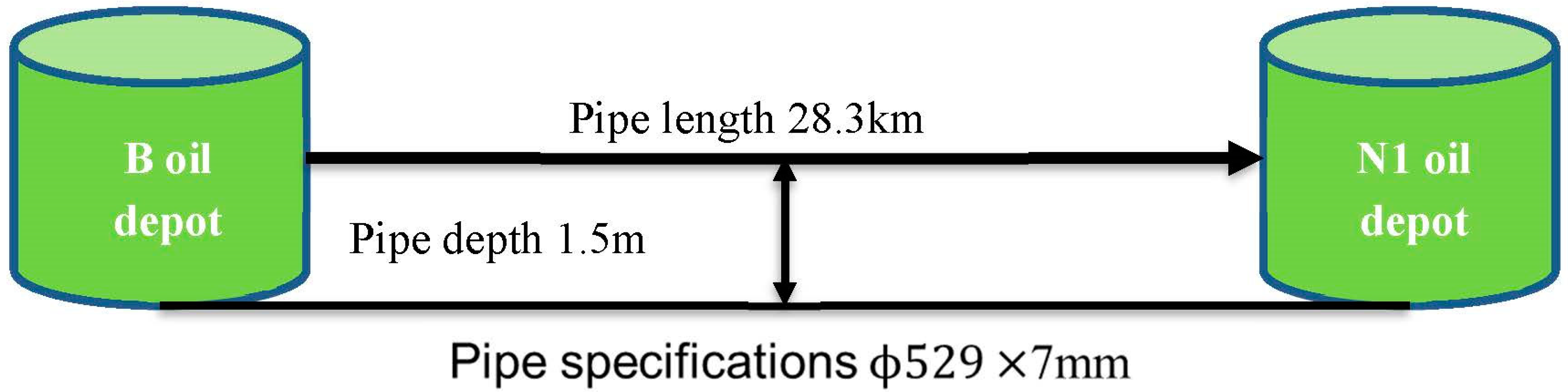
2.1. Brief Introduction of Pipeline Operation Condition

B oil depot was put into operation in December 1975, with a total of 10 oil storage tanks, 26 × 10⁴ m³ storage capacity, 6 oil transmission pumps, and 3 heating furnaces. The length of the external transmission pipeline from the B oil depot to the N1 oil depot after reconstruction in 2017 is 28.3049 km, with external transmission pipeline specification φ529 × 7 mm and design pressure 6.4 MPa. There is no insulation between the B oil depot and the seven-kilometer cut-off point 21.4869 km outside the N1 oil depot. There is insulation between the seven-kilometer cut-off point outside the N1 oil depot and the 6.818-km N1 oil depot. External pipeline design annual transmission capacity is 1000 × 10⁴ t/a. Schematic diagram of the oil pipeline of the B-N1 oil depot is shown in Figure 1.

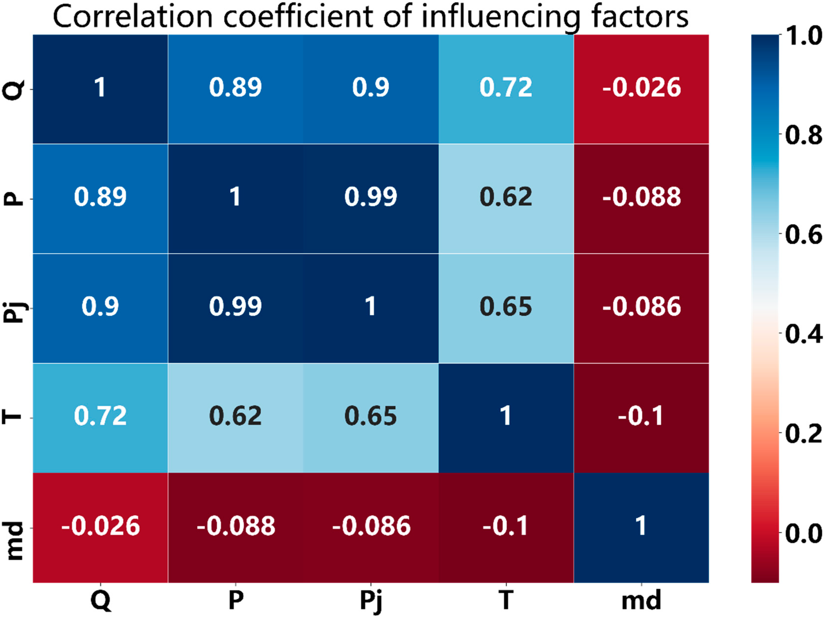
2.2. Analysis of Influencing Factors

During the operation of oil pipelines, the pressure drop is mainly affected by the friction loss along the pipeline, local friction loss, and elevation loss. The formula is as follows:

$$\mathrm{H}={\mathrm{h}}_{\mathrm{f}}+{\mathrm{h}}_{\mathsf{\zeta }}+({\mathrm{Z}}_{\mathrm{m}}-{\mathrm{Z}}_{\mathrm{c}})$$

(1)

In the formula: H is pipe pressure drop (m); ${\mathrm{h}}_{\mathrm{f}}$ is the friction loss along the pipeline (m); ${\mathrm{h}}_{\mathsf{\zeta }}$ is the total local friction loss (m); ${\mathrm{Z}}_{\mathrm{m}}$ is end elevation (m); ${\mathrm{Z}}_{\mathrm{c}}$ is initial point elevation (m).

For the selected pipeline, the elevation at the end of the starting point has been fixed, and the total local friction loss is generally 1–2% of the friction loss along the pipeline. Therefore, the elevation at the end of the starting point and the total local friction loss are not considered in the selection of input parameters [9]. Darcy’s formula is as follows:

$${\mathrm{h}}_{\mathrm{f}}=\mathsf{\lambda }\frac{\mathrm{L}}{\mathrm{D}}\frac{{\mathrm{v}}^2}{2\mathrm{g}}$$

(2)

In the formula: $\mathsf{\lambda }$ is hydraulic friction coefficient; $\mathrm{D}$ is pipe diameter (m); $\mathrm{L}$ is pipe length (m); $\mathrm{v}$ is flow velocity (m/s); $\mathrm{g}$ is acceleration of gravity (m/s²).

Among them, the friction along the path can be seen from the Darcy formula that is related to the influencing factors such as hydraulic friction coefficient, pipe length, pipe diameter, and flow velocity. The determination of hydraulic friction coefficient is closely related to Reynolds’ number, which is associated with mass flow and viscosity. Finally, it is determined that the friction along the way is related to the mass flow, viscosity, pipe diameter, and pipe length.

For a fixed pipeline, its type of conveying oil is single, and its viscosity is only affected by temperature. Therefore, only temperature is considered in the analysis of influencing factors, and viscosity is not considered. The length and diameter are fixed values, so they will not affect the calculation results. In this paper, the length and diameter are no longer selected as influencing factors of pressure drop calculation in training.

The correlation coefficients of the influencing factors include density, starting point pressure, flow rate, and starting point temperature selected for comprehensive analysis, mass flow (Q, unit ton/hour), endpoint temperature (T, units °C), density (md, units 10³ Kg/m³), and pressure drop from starting point to end point (pj, units MPa). Positive and negative values represent positive and negative correlations, respectively [10].

According to Figure 2, the correlation coefficient of the starting pressure P among the factors related to the pressure drop Pj is 0.99; secondly, for mass flow Q, the correlation coefficient is 0.9; the correlation coefficient of starting temperature T is 0.65. The correlation coefficient between density and pressure drop is −0.1, showing a negative correlation, so density is not considered when selecting the correlation analysis variables.

Finally, the relevant variables with a high correlation coefficient are: mass flow Q, starting pressure P, and starting temperature T, which are selected as the input values, and pressure drop Pj, taken as the output value for the training of the PSO-BP pressure drop model.

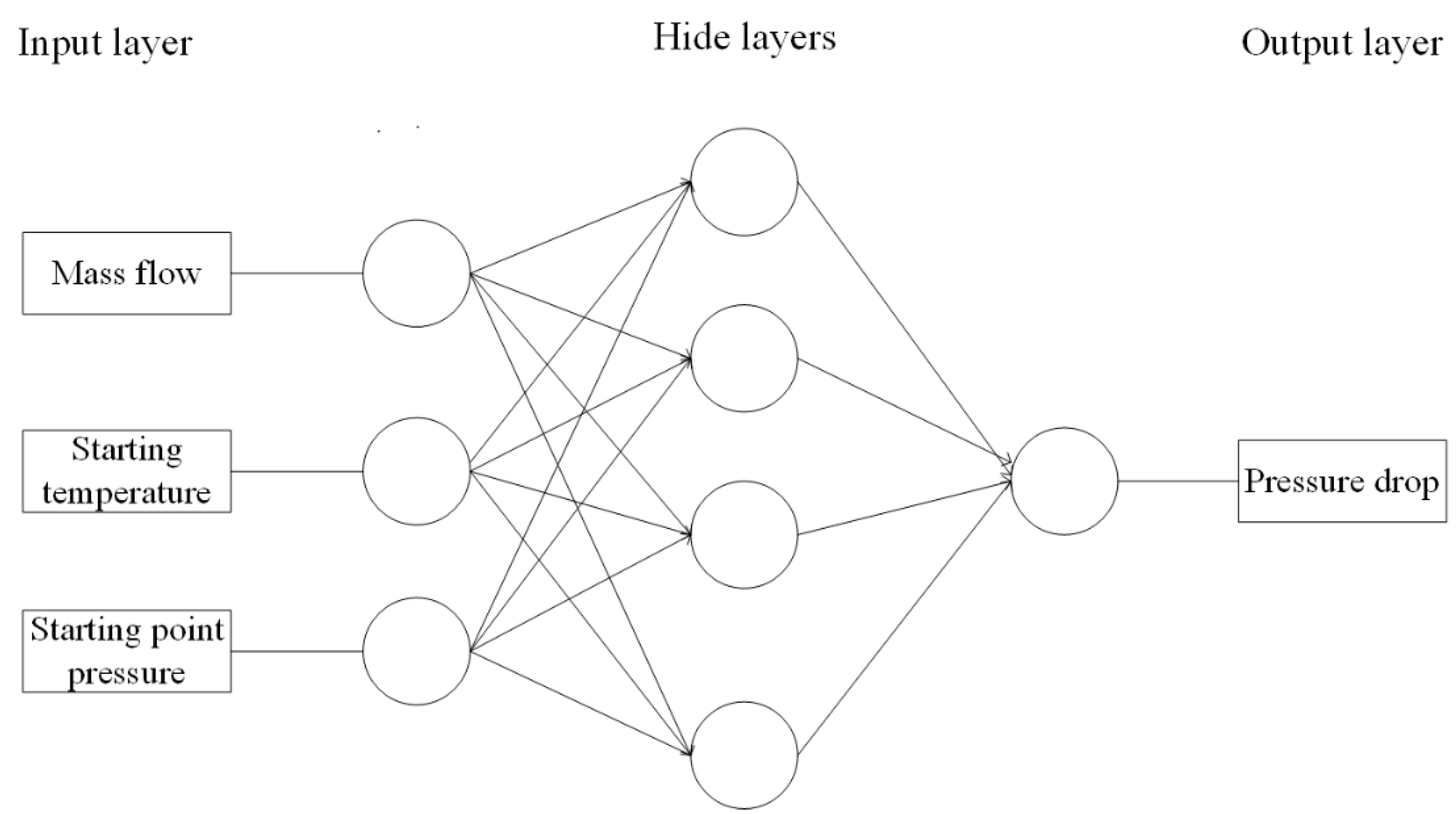
3. BP Algorithm Model

In BP neural networks, forward propagation is the process of forwarding computation based on the input layer to the output layer [11]. Reverse propagation is the reverse data flow after the result is deviated from the target value due to forward propagation [12]. Alternating data flow in both directions. The output between the neurons in each layer behind the input layer is obtained by forwarding propagation. The weights are updated after backward propagation. Finally, the machine learning process is completed [13]. The traditional B-P neural network model is shown in Figure 3.

BP neural network algorithm belongs to the gradient descent algorithm of error, that is reversing the weight parameter repeatedly advances a distance until the gradient is close to 0, at which time the parameter exactly produces the lowest value of error [14]. The error between the actual pressure drop value of the pipe and the output value of the BP neural network model is compared during the field test. This is performed by setting the iteration termination condition, dividing the test set and training set, and checking the training accuracy by the test set [15].

BP pressure drop model consists of a three-layer BP neural network, with mass flow rate, starting temperature, and starting pressure as input and pressure drop as output [16]. The number of neurons in the hidden layer is 7, and the solver function selects Adam (weight-optimized solver), the conductive activation function selects Relu, the maximum number of network iterations is set to 500, and the learning accuracy is set to 0.001 [17].

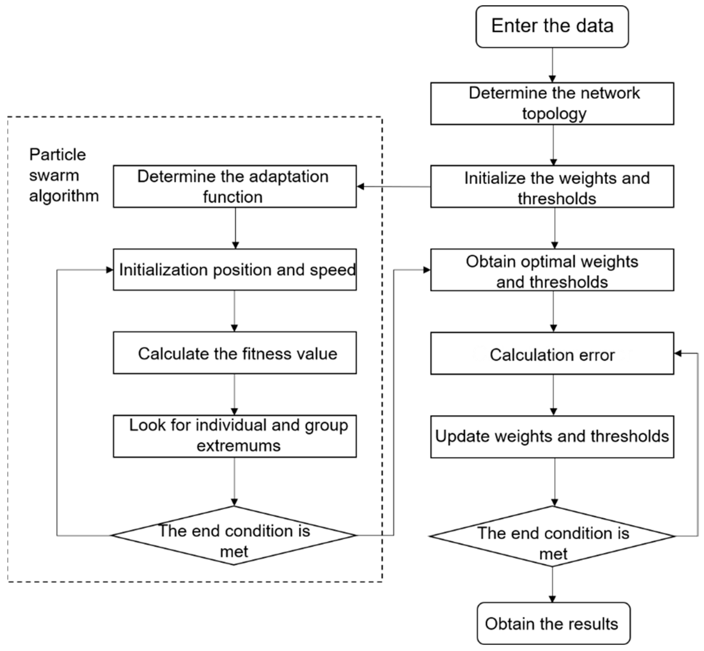
4. Optimized PSO-BP Neural Network Pressure Drop Model

PSO-BP Algorithm

The BP neural network has low global search capability and high local search capability, in contrast to the particle swarm algorithm which has high global search capability and low local search capability, from which the PSO-BP neural network mechanism can be constructed [18,19].

The basic idea of the particle swarm algorithm is to initialize random particles (random solutions) and then update them by an iterative process to find two extreme values. One is the optimal solution found by the particle itself, the individual extremum; the other is the current optimal solution in the whole population, the global extremum [20].

Assuming that the number of particle swarm is P, the position of the kth particle in D-dimensional space is expressed as $x_k=\left(x_{k1},x_{k2},\cdots ,x_{kD}\right)$. Flight speed is expressed as $v_k=\left(v_{k1},v_{k2},\cdots ,v_{kD}\right)$. The fitness function corresponding to each particle is $f\left(x_k\right)$; the individual extremum searched by this particle k is $p_k=\left(p_{k1},p_{k2},\cdots p_{kD}\right)$. The global extremum of particle swarm search is $p_g=\left(p_{g1},p_{g2},\cdots ,p_{gD}\right)$. Each particle in the population approaches the optimal position $f\left(x_k\right)$. Iteration speed and position according to the formula:

$$\begin{array}{l}{v}_{ij}^{t+1}=w{v}_{ij}^t+c_1{r}_1\left(p_{ij}^t-x_{ij}^t\right)+c_2{r}_2\left(p_{gj}^t-x_{xj}^t\right)\\ \end{array}$$

(3)

$$x_{ij}^{t+1}=x_{xj}^t+v_{ij}^{t+1}$$

(4)

In the formula $i=1,2,\cdots ,N$; $j=1,2,\cdots ,D$ is the dimension of particles; $t$ is the number of iterations; $c_1$, $c_2$ as a learning factor; $r_1$, $r_2$ is a random number between [0, 1], $\omega$ is used for inertia weight.

According to Formula (1), it can be seen that the particle’s iterative speed by constantly approaching the optimal solution, the inertia weight $\omega$, affects the iterative speed of the particle. The larger the inertia weight is, the stronger the global search and convergence ability is. The smaller the inertia weight is, the more emphasis is placed on the accurate search for local optimal values, which can be adjusted according to the actual situation. The adjustment method is as follows:

$$w=w_1-\frac{w_1-w_2}{T}·t$$

(5)

In the formula: $w_1$ is the initial weight, $w_2$ is used for termination weights, $T$ is the maximum number of iterations.

According to the basic idea of PSO, the specific process of PSO can be set as follows:

Step 1: Random particle initialization.

Step 2: Calculation of particle adaptation.

Step 3: For each particle, the fitness is compared with the optimal position that the particle has experienced, and the most suitable position is selected to replace it.

Step 4: For all particles, the fitness value is compared with the global optimal position, and the best position is selected to replace it.

Step 5: The velocity and position of the particles are changed to determine whether the iteration process needs to be carried out from step 2.

Combined with the characteristics of particle swarm optimization and the BP neural network algorithm, the weights and thresholds of the BP neural network are regarded as particles. The convergence speed and prediction accuracy of the BP neural network are determined by optimizing the position and speed of particles. The prediction steps of pipeline pressure drop are as follows:

(1) The parameters of the BP neural network and particle swarm optimization algorithm are set to determine the number, scale, learning rate, iteration number, and initial weight threshold of nodes in the input layer, hidden layer, and output layer of the BP neural network.

(2) Setting the mapping relationship between the PSO particle dimension and BP neural network weight threshold.

(3) Calculating fitness $f\left(x_k\right)$ is the mean square error between the actual calculated value and the field test value.

(4) According to the fitness function, the change of particle fitness value is compared, the iteration of individual optimal value is carried out, and the optimal global extremum is updated according to the fitness value of the particle swarm.

(5) Iterative particle position and velocity according to Formulas (4) and (5).

(6) Depending on the initial set of end iterations: the number of iterations reaches the set or the error meets the minimum requirement.

(7) The resulting optimal solution sets the weights and thresholds of the BP neural network, as well as the weights and thresholds of the BP neural network training and prediction.

The architecture diagram of the PSO-BP neural network pressure drop model is shown in Figure 4.

The PSO-BP pressure drop model flowchart is shown in Figure 5.

5. Calculation of Pipeline Hydraulic Pressure Drop

5.1. Calculation Examples

After collecting the mass flow rate, starting pressure, oil delivery temperature and other factors affecting the pressure drop, a total of 2791 sets of this pipeline data were selected, and some of the data were listed in

Table 1. Data table of the oil pipeline.

Mass Flow (ton/h)	Oil Temperature (°C)	Starting Pressure (MPa)	Density (103 Kg/m3)	Pressure Drop (MPa)
221.2128	51.25	0.97	0.8698	0.85
223.547	50	0.99	0.8688	0.87
268.3073	50.75	1.37	0.87	1.25
273.3313	51.25	1.37	0.8696	1.24
275.0043	51.25	1.37	0.8696	1.25
236.1731	57.5	1.23	0.8702	1.1
238.014	57.5	1.09	0.8694	0.96
236.354	53.5	1.1	0.8708	0.97
282.0318	54	1.49	0.8696	1.39
293.799	53.75	1.49	0.8695	1.38
292.2854	52.5	1.5	0.8692	1.39
291.7382	54	1.48	0.8686	1.36
289.9206	54	1.49	0.87	1.36
293.1723	54	1.5	0.8696	1.36
238.0784	52.75	1.05	0.8694	0.93
227.7555	52.5	1.05	0.8684	0.93
229.6628	52.5	1.04	0.8697	0.92
229.8628	52.25	1.05	0.8696	0.91
228.3393	52.5	1.05	0.87	0.93
228.1908	51.25	1.04	0.8686	0.92
189.0346	52.75	1.02	0.8706	0.9
225.1411	53	1.02	0.87	0.9
225.1944	53	1.02	0.8696	0.9
343.0175	53.75	2.17	0.8696	2.05
368.3538	53.25	2.18	0.8696	2.06
369.1735	54.5	2.14	0.8696	2.02
285.7059	53.5	1.01	0.8694	0.89
228.5625	53	1.02	0.8703	0.9
225.8829	53	1.02	0.8698	0.9
200.9451	50.5	0.97	0.8696	0.85
220.5551	51	0.99	0.8689	0.87
274.141	51.75	1.36	0.8688	1.24
273.0108	52	1.35	0.87	1.22
272.31	51.75	1.35	0.8697	1.23
262.0325	56.75	1.23	0.8696	1.1
236.9248	53.5	1.09	0.8696	0.96
237.3664	52.25	1.1	0.8696	0.97
290.5513	53.75	1.5	0.8715	1.4
290.4492	53	1.5	0.8697	1.39

, of which 80% were designated as the training set and 20% as the test set.

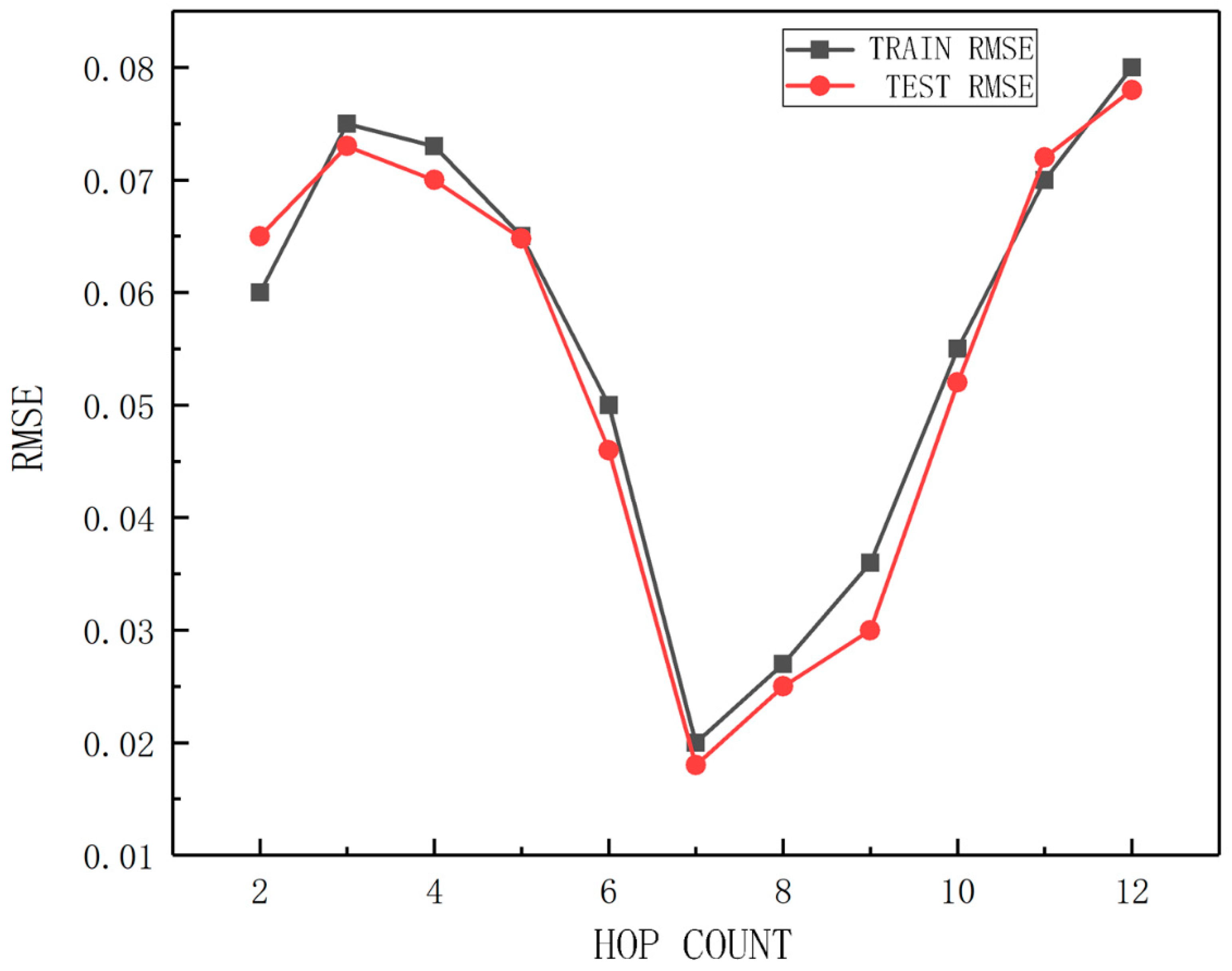
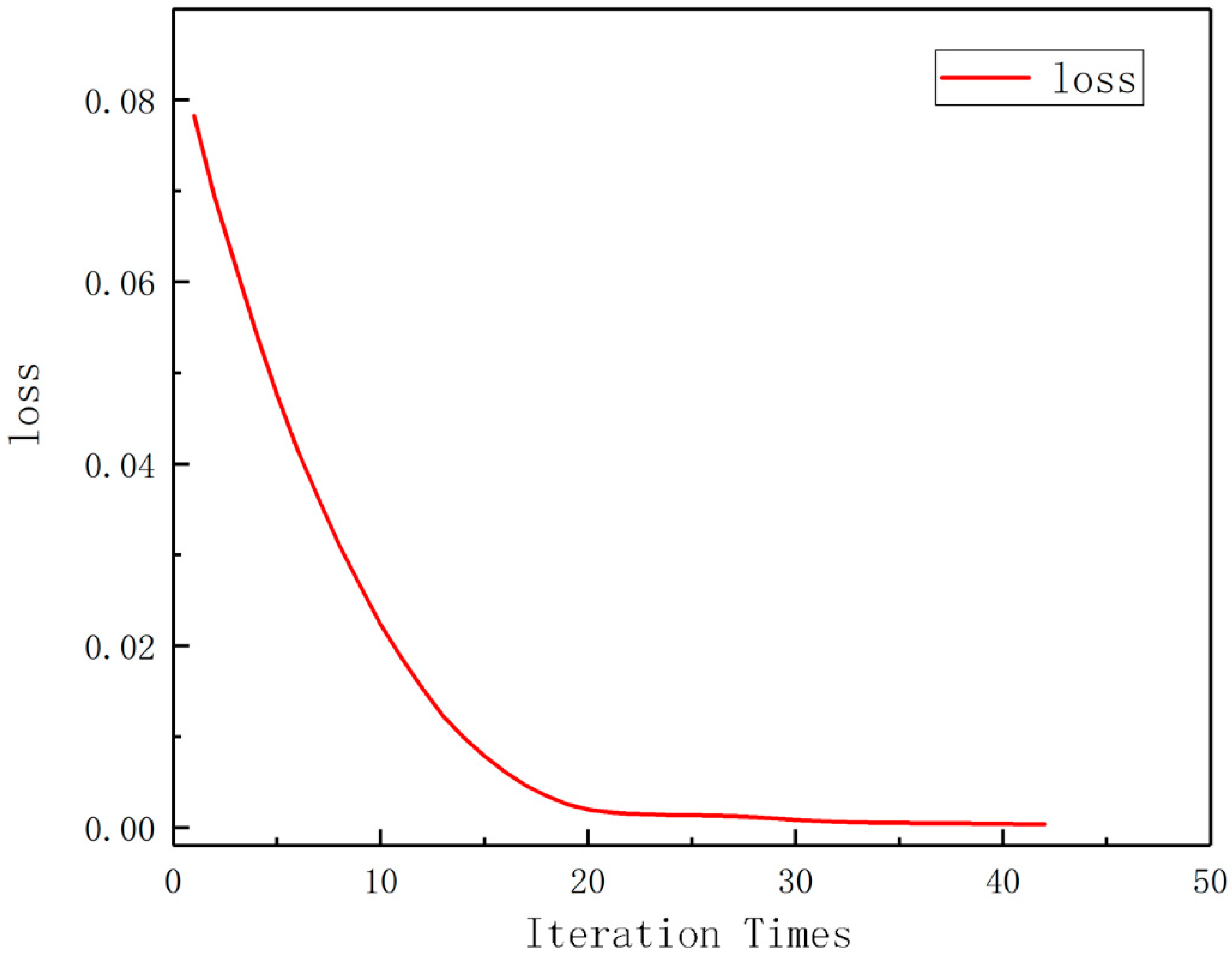
5.2. Construction of PSO-BP Pressure Drop Calculation Model

The input layer nodes of the PSO-BP pressure drop model are set as follows: mass flow, starting pressure and starting temperature of the oil. The output layer node is the pressure drop.

The number of hidden layer nodes in the BP model can be selected according to the formula as follows [1]:

$$n_1<\sqrt{(m+n)}+c$$

(6)

In the formula:

$n_1$: is the number of hidden layer nodes.

$m$: is the number of input layer nodes.

$n$: is the number of nodes for the output layer.

$c$: is the constant between 0 and 10.

According to Formula (6), the range of node numbers in this layer is (2, 13).

After many training comparisons, the relationship between the PSO-BP model error and the number of nodes in different hidden layers is shown in Figure 6 as follows.

As can be seen from Figure 6, within the results calculated by the empirical formula, the root mean square error at the beginning decreases with the increase of the number of nodes in the hidden layer, because the amount of effective information obtained between neurons is less when the number of elected nodes is small, resulting in a larger error. When the number of hidden layer nodes is 7, the root mean square errors of the test set and the training set are the smallest. With the increase in the number of selected nodes, the error is on the rise, which may lead to over-fitting and reduce the generalization ability of the model. Therefore, the number of nodes in the input layer is 2, the number of nodes in the hidden layer is 7, and the number of nodes in the output layer is 1. The optimizer is selected as Adam, and the effect is better on relatively large data sets. The activation function is Relu. The convergence rate is faster than that of Sigmoid and tanh functions, and there is no gradient saturation, which alleviates the occurrence of overfitting problem. Regularization was set to 0.001, initial learning rate was set at 0.1. We selected 20% of the pipeline data sets for the test set and 80% for the training set. Changes in LOSS values with iterations during training are shown in Figure 7, as follows.

As can be seen from the curves in the graph, loss is minimized after 42 iterations.

We used the PSO-BP model to calculate the training set sample distribution and RMSE and R² data as shown in Figure 8. The blue dots in Figure 8 is the predicted value of pressure drop.

The distribution of training samples and RMSE and R² values are shown in Figure 9 as follows. The blue dots in Figure 9 is the predicted value of pressure drop.

The pairing of the predicted and actual values of the pressure drop is shown in Figure 10.

According to the prediction results of pressure drop of the training set and test set data, the RMSE of the mean square error of the test set is 0.0232, and the RMSE of the mean square error of the training set is 0.0155. The R² of the training set and test set are 0.9910 and 0.9948.

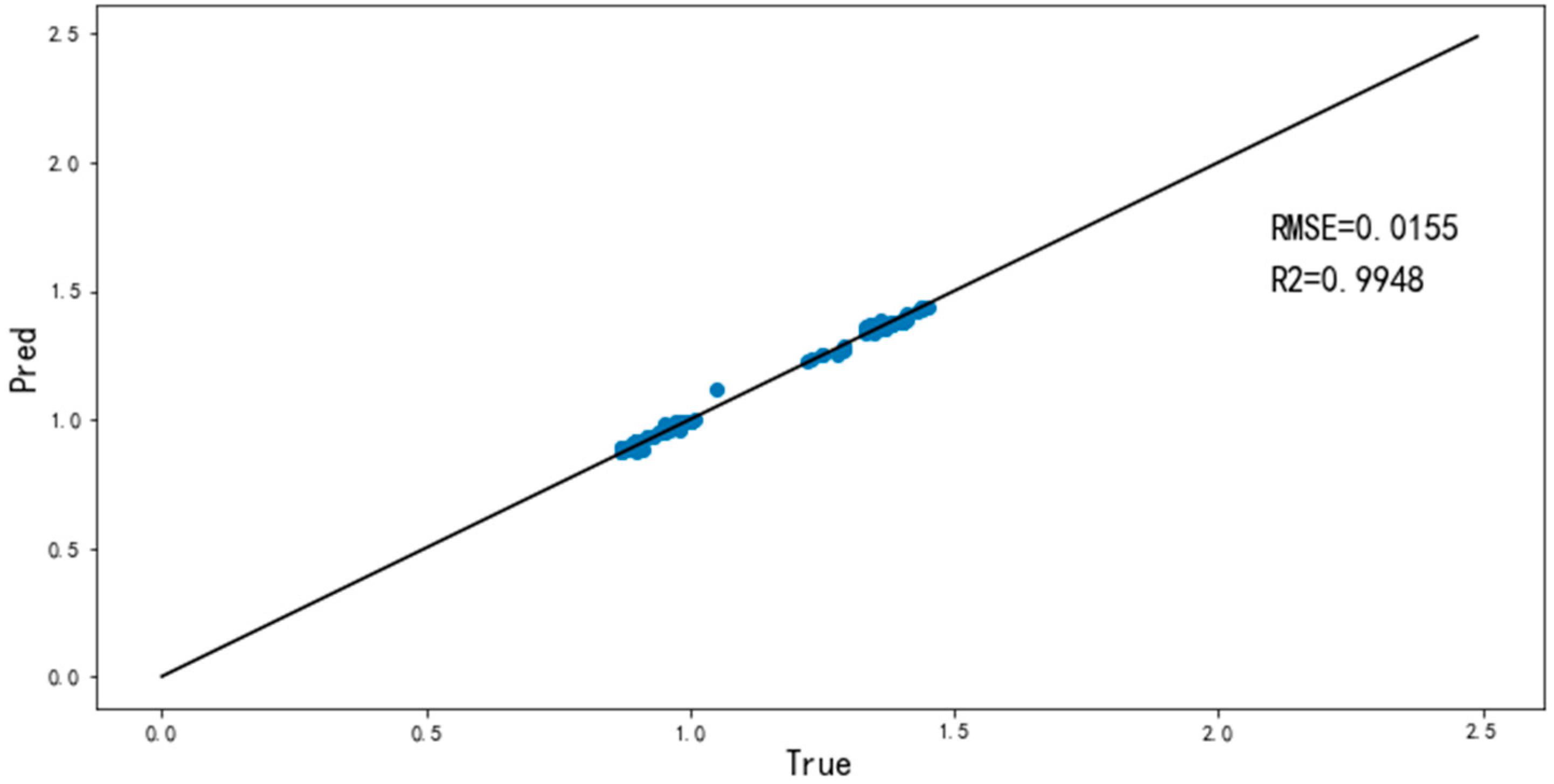
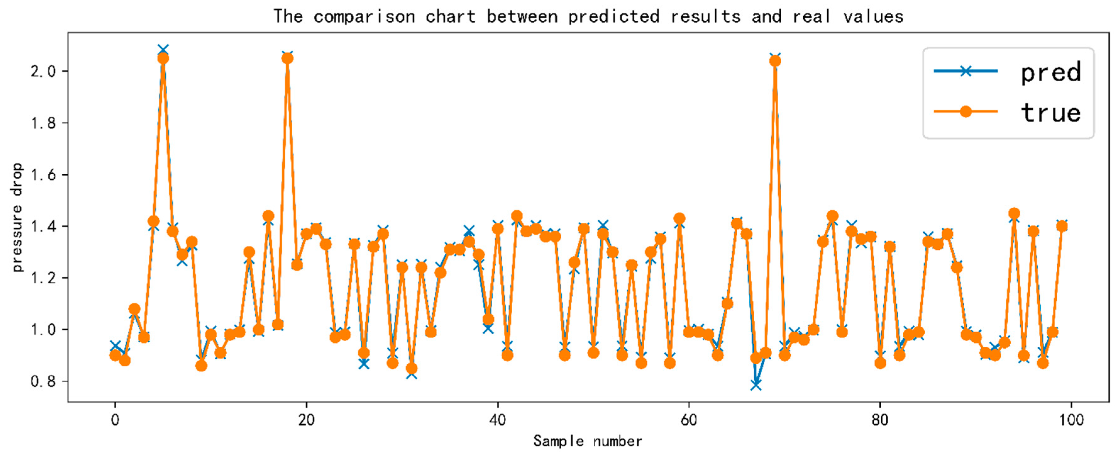
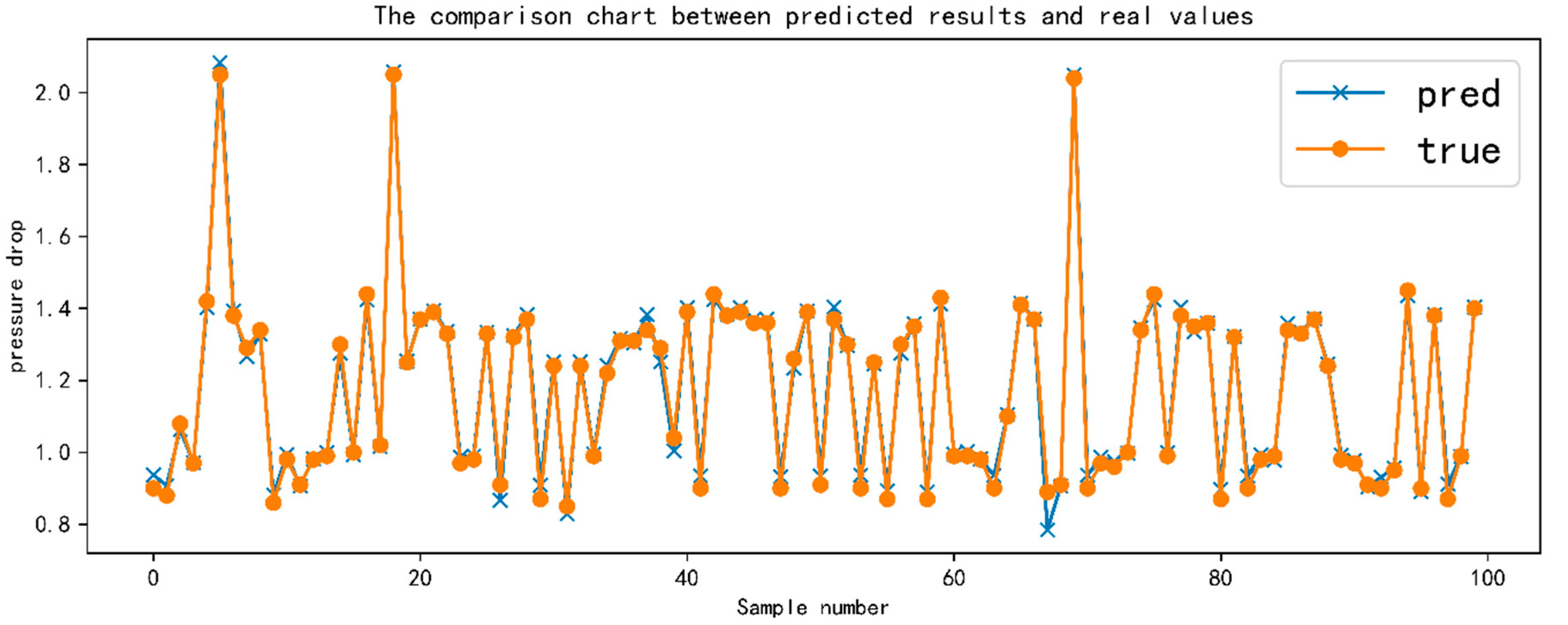
5.3. Comparative Analysis of Pressure Drop Calculation Results

According to the actual field data, the traditional BP model and PSO-BP model are trained, and the pressure drop is predicted.

The prediction results of the traditional BP model test set are compared with the real values as shown in Figure 11 as follows.

The prediction results of the optimized PSO-BP model test set are compared with the real values as shown in Figure 12 as follows.

According to the comparison of RMSE and R² data between the traditional BP pressure drop model and the PSO-BP pressure drop model, and the comparison of the predicted results and the real values, the calculation accuracy of the improved PSO-BP pressure drop model is significantly improved compared with the traditional BP pressure drop model.

6. Conclusions

The actual operation data of pipelines from the B oil depot to the N1 oil depot were collected. Based on the traditional calculation formula and the correlation coefficient thermal diagram, three main influencing factors affecting the pressure drop were selected: mass flow, starting pressure and starting temperature as input, and pressure drop as output. The traditional BP pressure drop calculation model and PSO-BP pressure drop calculation model were established.

Based on the BP neural network and the correlation coefficient thermal diagram, the traditional BP pressure drop model was established by adjusting the input and output nodes. Compared with the traditional pressure drop fitting calculation, the accuracy of the model was slightly improved. To accelerate the convergence rate and optimize the structure of the BP neural network, an improved PSO-BP pressure drop calculation model was established by combining the adaptive improvement of the BP neural network with the particle swarm optimization (PSO) algorithm. The measured verification set was selected for calculation and comparison between the models. The results show that the improved PSO-BP pressure drop calculation model has the highest accuracy. Compared with the traditional BP model, the convergence speed increased by 61.5%, the average absolute error was 0.02 MPa, and the average relative error was reduced by 13.16%, which improved the accuracy of the pipeline’s pressure drop prediction. The test verified that the PSO-BP pressure drop calculation model has high prediction accuracy for the pressure drop of fixed pipelines without considering the pipe length and diameter.

References

1. Cai, R.H.; Cui, Y.X.; Xue, P.J. The determination method of hidden layer node number of three-layer BP neural network. Comput. Inf. Technol. 2017, 25, 29–33. [Google Scholar]
2. Guo, Y.; Xiong, G.; Zeng, L.; Li, Q. Modeling and Predictive Analysis of Small Internal Leakage of Hydraulic Cylinder Based on Neural Network. Energies 2021, 14, 2456. [Google Scholar] [CrossRef]
3. Han, W.; Nan, L.; Su, M.; Chen, Y.; Li, R.; Zhang, X. Research on the Prediction Method of Centrifugal Pump Performance Based on a Double Hidden Layer BP Neural Network. Energies 2019, 12, 2709. [Google Scholar] [CrossRef]
4. Sun, T.; Huang, X.; Liang, C.; Liu, R.; Huang, X. Prediction and Analysis of Dew Point Indirect Evaporative Cooler Performance by Artificial Neural Network Method. Energies 2022, 15, 4673. [Google Scholar] [CrossRef]
5. Li, S.B. Research on Online Simulation and Operation Optimization Technology of Long-Distance Hot Oil Pipeline; Tianjin University: Tianjin, China, 2016. [Google Scholar]
6. Alpine; Qian, C.; Zhang, P.; Zhang, Y.; Zeng, L.; Tian, W. Based on the improved BP neural network prediction model of pipeline energy consumption. Oil Gas Storage Transp. 2014, 33, 869–872. [Google Scholar]
7. Hou, L.; Xu, X.; Cui, J.; Shi, Y. Energy consumption prediction method of oil pipeline based on BP neural network. Energy Sav. Technol. 2009, 27, 401–406. [Google Scholar]
8. Li, J.H.; Sun, S.C.; Cui, L. Leakage point location and experimental study of long-distance pipeline based on BP neural network principle. Eng. Mech. 2010, 27, 169–173. [Google Scholar]
9. Li, X. Data Mining Algorithms Based on Data Preprocessing and Regression Analysis and Their Applications; Lanzhou Jiaotong University: Lanzhou, China, 2014. [Google Scholar]
10. Qin, K.; Changqing, Y.; Yun, S. Research on data preprocessing methods under big data. Comput. Technol. Dev. 2018, 28, 1–4. [Google Scholar]
11. Stanley, K.O.; Clune, J.; Lehman, J.; Miikkulainen, R. Designing neural networks through neuroevolution. Nat. Mach. Intell. 2019, 1, 24–35. [Google Scholar] [CrossRef]
12. Nikolaus, K.; Tal, G. Neural network models, and deep learning. Curr. Biol. 2019, 29, 11–19. [Google Scholar]
13. Zhang, H.; Tian, Z. Failure analysis of corroded high-strength pipeline subject to hydrogen damage based on FEM and GA-BP neural network. Int. J. Hydrogen Energy 2022, 47, 14–35. [Google Scholar] [CrossRef]
14. Xu, B.; Dan, H.C.; Li, L. Temperature prediction model of asphalt pavement in cold regions based on an improved BP neural network. Appl. Therm. Eng. 2017, 120, 568–580. [Google Scholar] [CrossRef]
15. Ling, X.; Xu, L.S.; Yu, J.P.; Liang, R. The prediction of corrosion rate in oil pipeline based on improved BP neural network. Sens. Microsyst. 2021, 40, 124–127. [Google Scholar]
16. Yang, A.H.; Qing, P.; Liu, G.Z. BP algorithm fixed learning rate does not converge cause analysis and countermeasures. Syst. Eng. Theory Pract. 2002, 12, 22–25. [Google Scholar] [CrossRef]
17. Jiang, Y.J.; Ning, L.; Dao, H. Application of BP network with modified initial weights in CSTR fault diagnosis. J. East China Univ. Technol. 2004, 30, 207–210. [Google Scholar]
18. Zhou, H.; Sun, G.; Fu, S.; Liu, J.; Zhou, X.; Zhou, J. A big data mining approach of pso-based bp neural network for financial risk management with iot. IEEE Access 2019, 7, 154035–154043. [Google Scholar] [CrossRef]
19. Sun, B.C. The Residual Strength Prediction of Corroded Pipelines is Based on an Improved BP Algorithm and Genetic Algorithm; Lanzhou University of Technology: Lanzhou, China, 2011. [Google Scholar]
20. Wang, J.; Jiao, J.; Yu, H.; Chen, Z.; Yu, B. Energy consumption optimization method for crude oil pipeline system based on swarm intelligence optimization. Oil Gas Storage Transp. 2022, 41, 1–9. [Google Scholar]
Figure 1. Schematic diagram of the oil pipeline.
Energies 15 05880 g001
Figure 2. Correlation coefficient analysis of influencing factors.
Energies 15 05880 g002
Figure 3. Pressure drop model of traditional BP neural network.
Energies 15 05880 g003
Figure 4. PSO-BP neural network pressure drop model.
Energies 15 05880 g004
Figure 5. Flow chart of PSO-BP pressure drop model.
Energies 15 05880 g005
Figure 6. Graph of relationship between nodes and errors.
Energies 15 05880 g006
Figure 7. Loss curve of PSO-BP pressure drop model.
Energies 15 05880 g007
Figure 8. RMSE and R2 of the training set.
Energies 15 05880 g008
Figure 9. The test set RMSE and R2.
Energies 15 05880 g009
Figure 10. Comparison of predicted and real values.
Energies 15 05880 g010
Figure 11. Prediction comparison chart of traditional BP pressure drop model.
Energies 15 05880 g011
Figure 12. Prediction comparison chart of PSO-BP pressure drop model after optimization.
Energies 15 05880 g012