Abstract
There is increasing growth in load demands and financial strain to upgrade the present power distribution system. It faces challenges such as power losses, voltage deviations, lack of reliability and voltage instability. There is also a sense of responsibility in the wake of environmental and energy crises to adopt distributed renewable resources for power generation. These challenges can be resolved by optimally allocating distributed generators (DGs) at different suitable locations in the radial power distribution system. Optimal allocation is a non-linear problem which is solved by powerful metaheuristic optimization algorithms. In this work, an objective function is introduced to optimally size four different types of DGs by utilizing honey badger algorithm (HBA), and comparison is drawn with grey wolf optimization (GWO) and whale optimization algorithm (WOA). The objective is to boost the voltage profile and minimize the power losses of the standard IEEE 33bus and 69-bus radial power distribution system. It is observed from the simulation results that honey badger algorithm is faster than grey wolf optimization and whale optimization algorithm in reaching accurate and optimum results in a mere one and two iterations for IEEE 33-bus and 69-bus systems, respectively. Additionally, power losses are reduced to 71% and 70% for IEEE 33-bus and 69-bus, respectively.
1. Introduction
The generation, transmission and distribution networks are the three basic pillars that support the electricity grid. The distribution component of the power system connects bulk-generated power with the consumers. It has low voltage levels and high current values. It is reported that an almost 13% loss of generated power occurs due to losses in the distribution system where the loss level target is around 7.5% [1]. The distribution system has a high power loss due to the R/X ratio being high at the lines and buses. Ideally, the real power loss would be within the range of 3–6%. This value reaches up to 10% in the case of developed and 20% for underdeveloped countries [2]. These losses can be divided into two categories, i.e., technical and non-technical. Technical losses may occur due to natural events, design malfunction, overloading and the type of material being used in the system, whereas power losses of a non-technical nature involve measurement, monitoring issues and power theft. Different techniques are deployed to reduce distribution power losses, including placement of bypass capacitors, demand side management, network reconfiguration and allocation of distributed generation. Distribution systems are usually designed to propagate power in a radial operation, hence posing challenges for the integration of renewable distributed generation resources [3]. It is observed that the introduction of capacitors and distributed generation units in the system improves the voltage profile and reduces the overall power loss. Optimum sizing of capacitor banks in IEEE 34 and 85 test bench systems with changing load from a low load value to the peak value is performed using bacterial foraging optimization algorithm (BFOA) [4]. Allocation of switched capacitors in the power distribution system by implementing a mixed integer linear model results in convergence of optimum solution [5]. The preference to deploy DGs in the modern power system versus bypass capacitors is because the reduction in power losses is double with the integration of DG units. Optimum installation of the capacitors at the right location can do the required task, but in recent times renewable resources such as photovoltaic (PV), wind and biogas can be installed more rapidly because of their ability to fulfil the load demand, thereby reducing power system congestion and losses. They work flexibly in both configurations, i.e., on-grid and off-grid.
The International Council on Large Electric Systems (CIGRE) defines DGs as power generation between 50 and 100 MW, whereas the Electric Power Research Institute (EPRI) terms it as power generation from a few kilowatts to 50 MW. DGs have both economic and technical benefits, i.e., improvement of system frequency, voltage improvement, fewer pollutants, increased security and efficiency, investment plans for facility upgrades and lower fuel prices [6]. Based on the kind of power generation, DGs may be sorted into four categories depending upon their ability to deliver or absorb active and reactive power to the system [7]. These DGs are categorized as follows:
- Type-1: DGs that only contribute to the real power in the system, e.g., fuel cells and photovoltaic systems.
- Type-2: DGs that only compensate the reactive power in the system, e.g., capacitors and reactive power compensators.
- Type-3: DGs that can contribute both active and reactive power to the system. The prime examples of these kinds of DGs are synchronous machines.
- Type-4: DGs that contribute active power but consume reactive power in the system, e.g., wind turbines.
The optimal allocation of DGs in the distribution system takes precedence. DG allocation is a non-linear problem that requires metaheuristic algorithms to calculate the suitable DG size. These algorithms are applied to solve complex real-life problems. Optimization problems are solved these days through global solutions in evolutionary techniques, i.e., genetic algorithms and particle swarm optimization [8,9]. Whale optimization is used to simultaneously minimize the real and reactive power in IEEE 33-bus and 69-bus systems by optimal DG sizing that improves system load factor and voltage profile [10]. Effective sizing of DGs with respect to power loss in the network is performed by using dragonfly [11], swarm moth flame [12], harmony search [13] and firefly optimization [14] algorithms. There are multiple metaheuristic algorithms that mimic the behavior of animals, e.g., artificial bee colony (ABC) [15], whale optimization algorithm (WOA) [16], grey wolf optimizer (GWO) [17] and honey badger algorithm [18]. A comparison of gravitational search algorithm (GSA) and improved gravitational search algorithm (IGSA) has been drawn for DG sizing, minimizing overall cost and enhancing voltage stability factors [13]. By installing DG type-1 into RDS in the best possible way, the manta ray foraging optimization algorithm (MRFO) was used to reduce active power loss [19]. Considering deterministic load demand and DG insertion in a distribution power system, a symbiotic organism search algorithm can be deployed in optimal DG siting to boost the voltage stability of the power system [20]. The optimal capacitor sizing problem in a radial distribution system is resolved using polar bear optimization algorithm (PBOA) in varied loading circumstances. The cost of real power loss and various costs related to shunt capacitors are integrated into the annual operating cost (AOC) by developing several objective functions [21]. Hybrid techniques are used to optimally size distributed generation by combining different methodologies simultaneously [22]. A hybrid methodology involving ε-constraints and a genetic algorithm generates a solution of non-inferior nature to give choices to planners to opt between different cost outputs [23]. A new hybrid algorithm involves the combination of optimal power flow (OPF) and D-PSO to allow distribution utilities to plan DGs optimally [24]. To reduce power losses, a hybrid method (MFO-SCA) based on moth-flame optimization and sine cosine algorithm optimizes a single objective function to introduce DGs and capacitors into the radial distribution system. Both algorithms are used to improve the exploitation and exploration stages, respectively [25]. To improve the thermal limits and voltage stability of the distribution system, a tabu search algorithm is used with the hybrid system of flexible AC transmission system and DGs [26]. Besides optimal sizing, suitable placement of DGs plays a crucial role in achieving the required attributes.
There are methodologies to allocate DG optimally that can be categorized as analytical, classical and metaheuristic algorithms. Analytical techniques were initially used to locate DGs in the distribution system. In an unbalanced distribution system, a novel analytical method [13] was utilized for the unbalanced feeder to solve for the DG allocation of type-4. Other analytical techniques are used [27,28] to find suitable locations for the DGs in networked as well as radial distribution systems. Even though analytical techniques are easy to use, they can only incorporate one objective and one DG at a time. For the best placement of renewable DG sources, a mixed-integer linear programming-based methodology was used. Classical optimization techniques are based on linear programming algorithms that are extensively used to allocate the distributed generation into a distribution system [29], but the MILP approach is challenging to comprehend and apply. Therefore, the location is determined through application of various metaheuristic algorithms [9,12,28]. To calculate a DG’s location for its allocation into the power distribution system, a backtracking search optimization algorithm which uses loss sensitivity factor and bus voltages is deployed [30]. DG and FACTs are also allocated by conventional, AI and optimization tools [31]. There are different indices, too, that have been introduced to calculate suitable locations for DG installation, including the voltage stability index (VSI), the power loss sensitivity index (PLSI) and the power stability index (PSI) [8,30]. There are many metaheuristic algorithms in the literature that are used to optimally site and size the DGs in a distribution system, as mentioned above. Mostly, these metaheuristic algorithms work in two stages, i.e., the exploitation and the exploration stage. Additionally, most modern metaheuristic algorithms have a low exploitation rate to find local solutions in the chosen sector and a high exploration rate to investigate the prospective area in the search space. Because of controlled randomized methods to identify the best global solutions and avoid the local solutions in the potential area, HBA contains a high exploration rate and maintains an adequate population diversity during the exploitation stage. The main contributions of this paper are as follows:
- Honey badger algorithm (HBA) is used to perform the sizing of the four types of DGs in IEEE 33-bus and 69-bus power distribution systems. To the best of the authors’ knowledge, no comparison has been drawn between IEEE 33-bus and 69-bus test bench systems using HBA.
- A backward/forward sweep load flow analysis is performed for the standard IEEE 33-bus and 69-bus distribution systems to determine the required variables for power loss index and optimization algorithms for optimal DG sizing and allocation, respectively.
- A comparative analysis is carried out for HBA, GWO and WOA to compare their accuracy and convergence time for achieving optimal results for IEEE 33-bus and 69-bus systems.
This paper presents an approach for optimal sizing and placement of four different types of DGs in IEEE 33-bus and 69-bus distribution systems. The sizing of the DG is performed using HBA with the help of an objective function that is based on the power losses where the placement of the DG is determined using power loss index method (PLI). The aim of the whole procedure is to minimize the power losses and boost the voltage profile and stability of the system. A comparison of the resulting accuracy and convergence time is drawn between HBA and other metaheuristic algorithms, i.e., GWO and WOA.
2. Backward/Forward Sweep Algorithm (BFS)
Backward/forward sweep (BFS) is a power load flow technique for radial networks [32]. Each iteration of the BFS requires two computing cycles. At each node, the voltage beginning from the reference node to the end nodes is calculated using the forward sweep. The current or power flow solutions start at the branch of the end nodes and move towards the branch connected to the reference node in the backward sweep. The voltage and current are maintained constant throughout the backward and forward sweep, respectively. The convergence of the power load flow is verified at each iteration. Figure 1 shows a cross-section of two buses in a radial power distribution system.
where is the current injection into node m and is the voltage at node . is the current of node , is the injection of current into the branch current matrix and is the current iteration value.
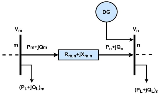
Figure 1.
A cross-section of two nodes and in a radial power distribution system.
In the first phase of the load flow analysis, the injection current at the nodes is calculated using Equation (1). Backward sweep is applied from the ending branch towards the base node using Equation (2). In the end, voltages are computed by applying forward sweep using Equation (3).
3. Power Loss Index Method (PLI)
In this method, a total reactive load is balanced at each bus to evaluate the loss reduction [33]. The normalization of power losses varies in a range of [0, 1]. The losses are divided into minimum and maximum loss reductions.
where is the real power beyond bus j, is the reactive power beyond bus j, is the resistance and is the reactance in the kth line. Likewise, is the loss reduction at bus (b), is the maximum reduction value and is the minimum reduction value. Active and reactive losses in a distribution power system are calculated with Equations (4) and (5). The loss reduction of a bus in comparison to minimum and maximum loss reduction (LR) of the system is called the power loss index (PLI) and it can be computed with Equation (6) The higher the index is, the higher is the loss reduction (LR) value of that bus and, hence, it is a more suitable location for DG allocation. To determine suitable DG locations, the PLI method is applied on the IEEE 33-bus and 69-bus test bench systems and the achieved optimum locations are at bus 30 and 61, respectively. In Table 1, the five most suitable buses are listed based on their higher PLI values.

Table 1.
Five most suitable buses for DG allocation based on higher PLI values.
4. Objective Function Formulations
Unlike transmission systems, there is high current and low voltage in the distribution system, due to which copper losses exist.
The copper losses are calculated using Equation (7) to evaluate the active losses in the system. Whereas shows the number of buses, is the current passing through the system having a resistance .
where and are the coefficients and are determined by Equations (10) and (11). and are the phase angles and is the resistance between bus and , respectively. The objective function in Equation (8) is formulated based on the active power loss of the system. In the first step, the load flow analysis is performed. After this, the objective function is inserted into each metaheuristic algorithm to calculate power losses at each iteration by using Equation (9) [34]. The losses decrease at every iteration and the size of the DG is updated as the algorithm approaches its final solution.
The limits for DG-1 are in kW, for DG-2 in kVAR and for DG-3 in kVA [33]. The constraints are given by Equations (12), (13) and (14), respectively.
5. Metaheuristic Algorithms
5.1. Honey Badger Algorithm
The honey badger algorithm imitates honey badger behavior [18]. It is placed in the category of a swarm-based metaheuristic optimization algorithm. A honey badger catches its prey by moving slowly and consistently while using its ability to smell the target. Through digging, it begins to locate the target’s location before grabbing it. It can make up to fifty holes and cover a distance of forty kilometers in a day to find food. Although honey badgers enjoy eating honey, they have trouble finding beehives themselves. To find beehives, honey badgers follow the honeyguide bird and then open the beehives with their claws. In this way, they both help each other and enjoy the honey.
Here and are the upper and lower bound, and is a random number which varies between 0 and 1. By using Equation (15), the position of the honey badger is determined.
where and are the strength of the source of smell and the spacing between the honey badger and its target, which are calculated by Equations (17) and (18). is a random number which varies between 0 and 1. The concentration strength of the target and the spacing between the target and the honey badger are linked to intensity . If the intensity of smell is high, the movement of the honey badger towards the target is fast, and vice versa. Intensity of smell is calculated by Equation (16).
To guarantee a seamless transition from exploration to exploitation, the density factor () regulates time-varying randomness and is calculated by Equation (19) where is the maximum number of iterations and C is a constant.
5.1.1. Digging Mode
In this mode, the honey badger smells the target and gets close to the target position by using its smelling ability. When it gets close to the target, it starts digging to catch the target.
where is the location of the target, is a constant which is its ability to find food, is the spacing between the honey badger and its target, , and are random numbers between 0 and 1, and F acts as the flag to alter the direction of search. The digging mode is depicted through Equation (20).
5.1.2. Honey Mode
In honey mode, to locate the honey beehive the badger takes aid from the honeyguide bird and follows its path.
where is the new position of the honey badger and is the target’s location. The honey badger changes its position by following Equation (21). As this involves both the exploration and the exploitation phases, it performs a global search. Figure 2 explains the working of the HBA algorithm in detail.
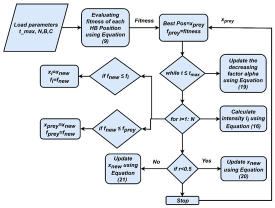
Figure 2.
Execution framework of HBA.
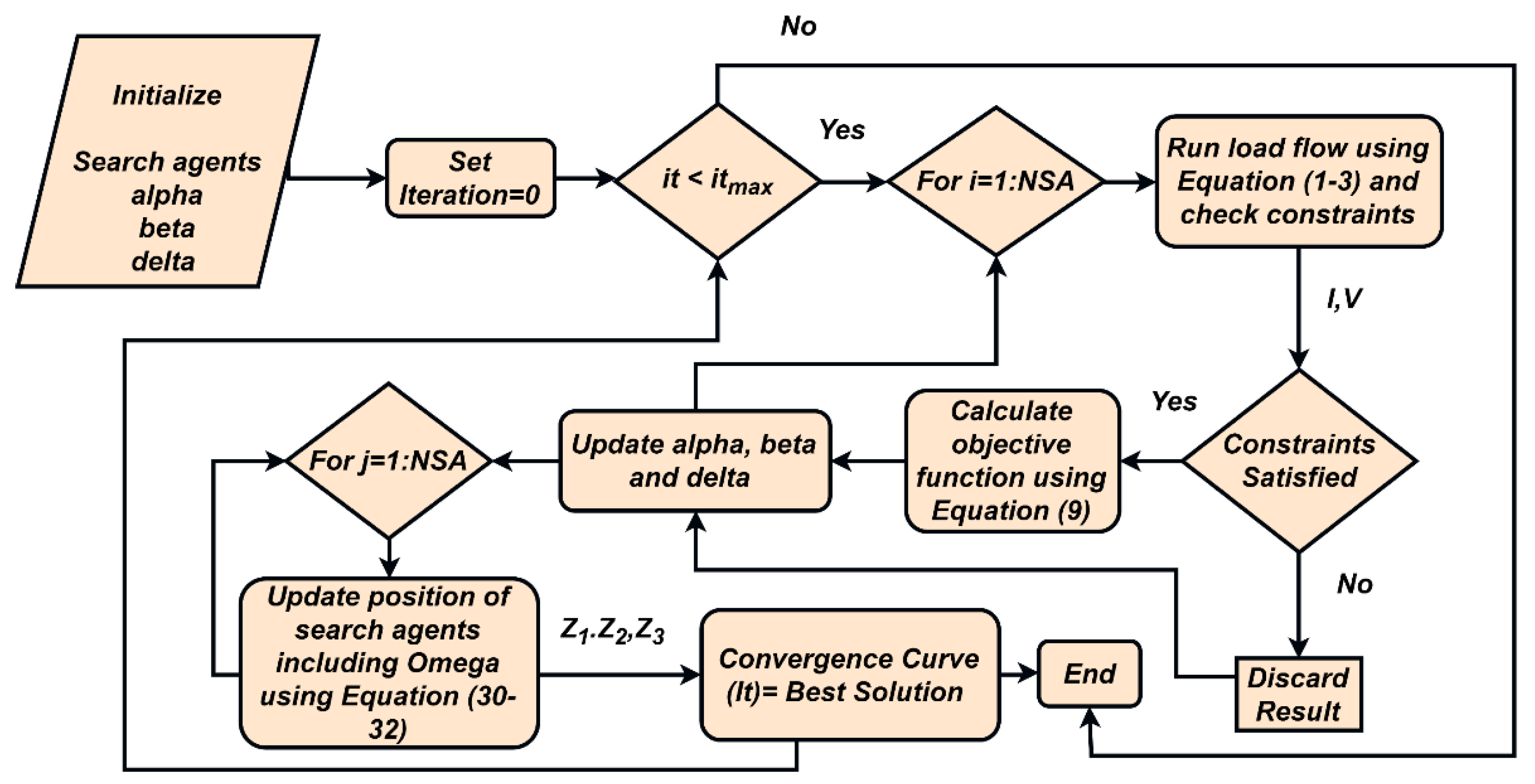
5.2. Grey Wolf Optimization Algorithm
The GWO algorithm is a population-based algorithm that works using the mechanism and hierarchy of leadership among grey wolves, which live in packs of five to twelve members and follow a social ranking [17]. The ranking starts from α and moves down to ω. The α of the pack is at the top of the ranking and makes all the decisions about hunting, sleeping, waking and staying in a certain place. The β of the pack is the second highest level and is the subordinate of the α. They reinforce the commands of α and give feedback to help it make sound decisions. The δ of the pack reports to the α and the β, whereas the ω are to merely follow the orders.
Encircling and Hunting Prey
The grey wolves coordinate in a pack and circle around their prey. In a pack of grey wolves, the α, β and δ know the best position of the prey and the ω are compelled to follow the position of wolves higher to them in social ranking.
where represents the current iteration, is the position vector of the grey wolf and is the position vector of prey. The behavior of the encircling of the wolves around their prey is represented by Equations (22) and (23). The ω update their position by Equation (24). Figure 3 displays the execution procedure of the GWO algorithm.
where , , , , , , are presented from Equations (25)–(32). Here are coefficient vectors.
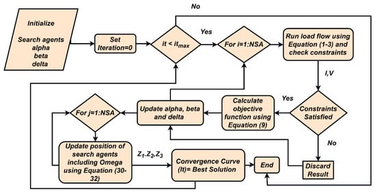
Figure 3.
Execution framework of GWO.
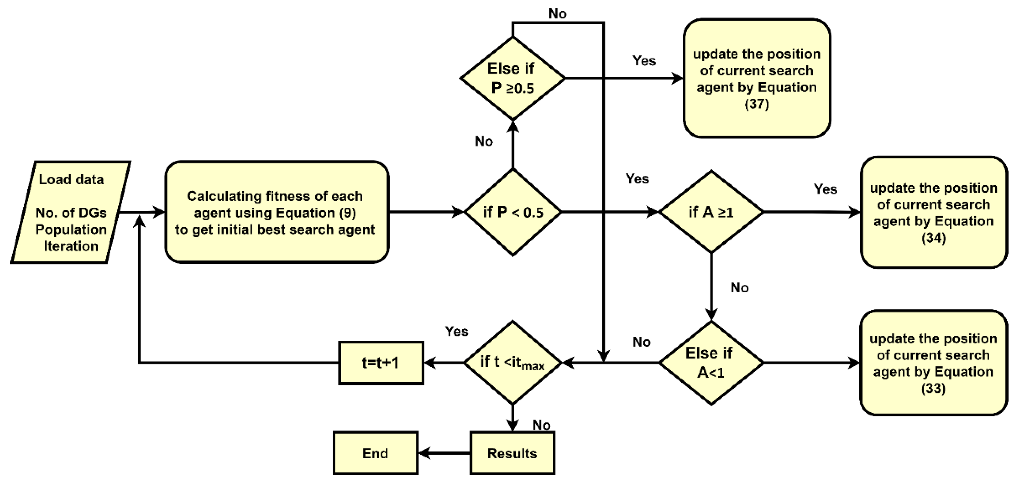
5.3. Whale Optimization Algorithm (WOA)
WOA is based on the movement of whales [16]. The bubble net feeding method mimics the hunting behavior of humpback whales. First, the whales encircle their prey, then they hunt them using the bubble net feeding method and reach the prey accurately with the help of their unique search strategy.
5.3.1. Encircling and Hunting Prey
The humpback whales circle around their prey by considering the initial position as the current best solution and upgrade their location from the initial position.
Here t is the present iteration and A, C are the coefficient vectors that are calculated from Equations (35) and (36), whereas denotes the position vector. The upgradation of location from the initial position is done using Equations (33) and (34). is the best optimized solution with being the best location found so far. As the iteration progresses, decreases linearly from 2 to 0 and represents a random vector.
5.3.2. Bubble Net Attacking Method
Two different mechanisms, the shrinking encircling mechanism and the spiral updating position, can be analyzed to model a given method of attacking.
In this attacking method, a spiral Equation (37) is used to imitate the movement of whales in a helix shape. There exists a probability () of 50% to work between both the attack strategies using the bubble net method. During the exploration, to find prey, the search agent’s location is chosen randomly rather than opting for the best agent, and this enables the WOA algorithm to work towards a global search solution. Figure 4 depicts the functioning of the WOA algorithm.
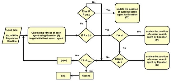
Figure 4.
Execution framework of WOA.
6. Simulation Results and Discussion
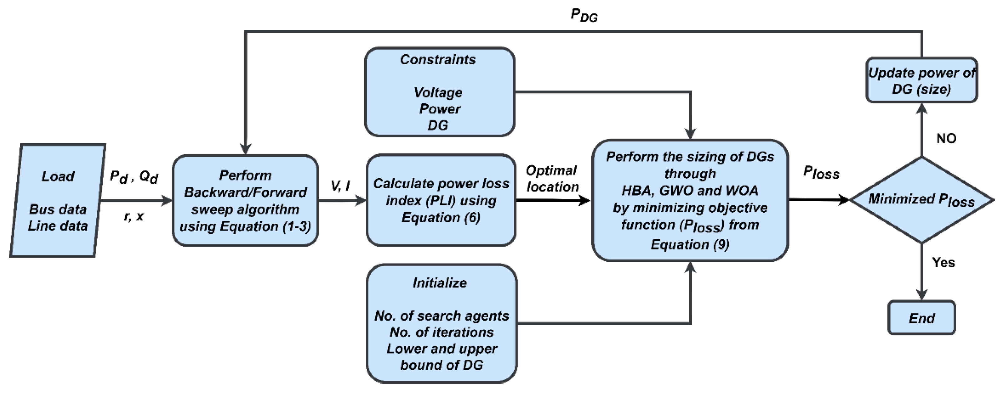
Three metaheuristic optimization algorithms HBA, GWO and WOA are applied on IEEE 33-bus and 69-bus radial distribution systems to optimally size where the PLI index is used for the suitable placement of DGs. For this objective, an optimization method is defined in MATLAB to minimize the power loss of the system as shown in Figure 5. In the initial step of the optimization procedure, the line and bus data are loaded giving us the active power demand () and the reactive power demand () of the buses with the reactance () and resistance () of the line. In addition to this, a backward/forward sweep load flow analysis is performed on an IEEE 33-bus distribution system which calculates the bus voltages and branch currents. The optimal locations of the DGs are calculated through the PLI method by using Equation (6). These optimal locations, with the combination of constraints and initialized variables shown in Figure 5, are inserted into the optimization algorithms to perform the optimal sizing of DGs. Initially, the DG value is randomly chosen within the bounds of the constraints mentioned in Equations (12)–(14). This DG is inserted into the suitable location provided by the PLI method and the power losses of the system are computed using the objective function in Equation (9). If the power losses are minimized, the system returns a DG value which is an optimal size to allocate in the system. Otherwise, the DG value is updated, and the process of load flow analysis is performed again repeating the cycle until the value is minimized or the iteration criteria are met.
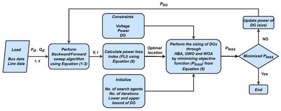
Figure 5.
A schematic diagram representing the whole optimization process for optimal allocation of DGs in a distribution power system.
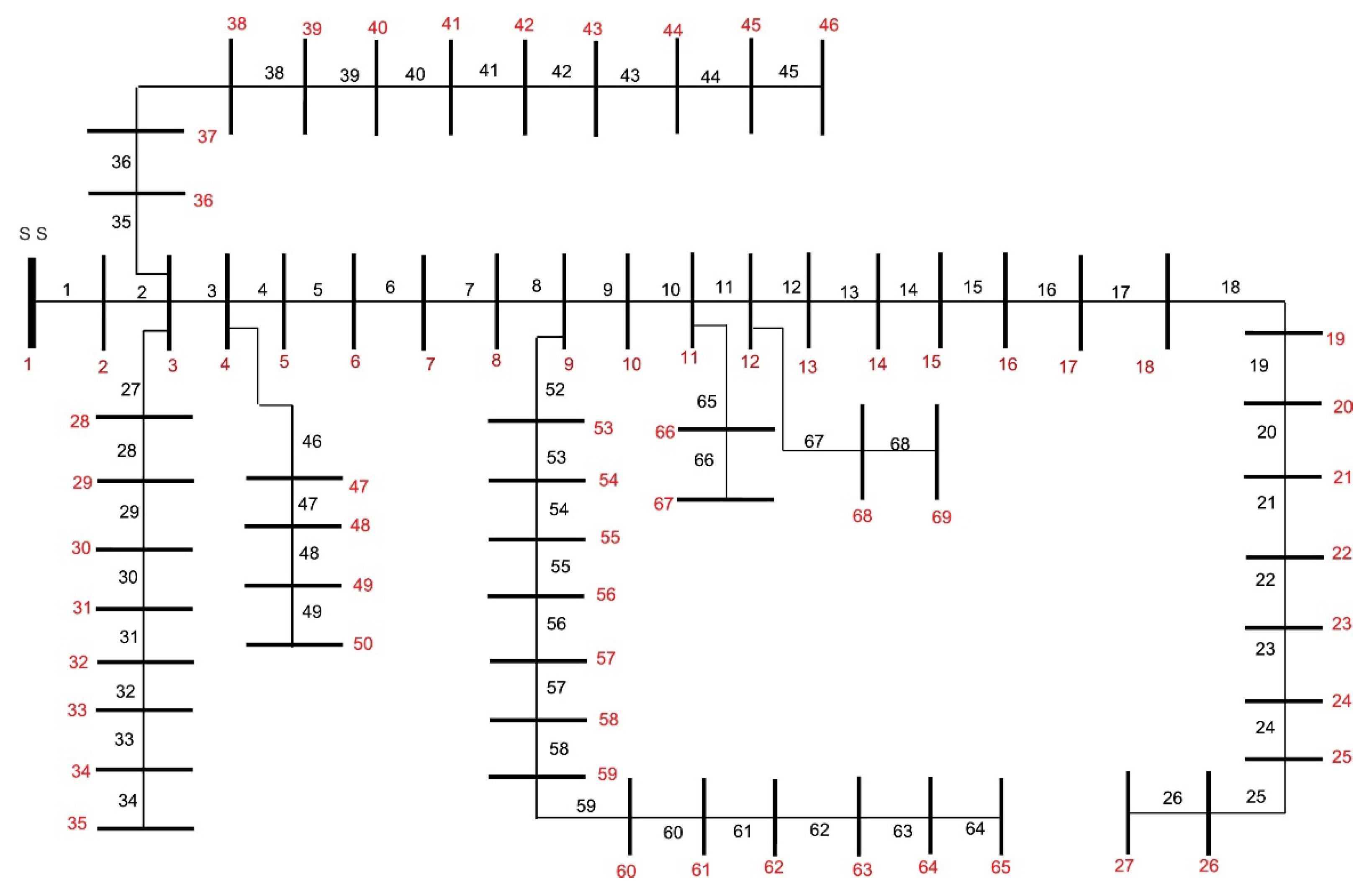
IEEE 33-bus and 69-bus radial distribution systems are shown in Figure 6 and Figure 7. The voltage constraints of the systems are between 0.95 (p.u) and 1.05 (p.u).
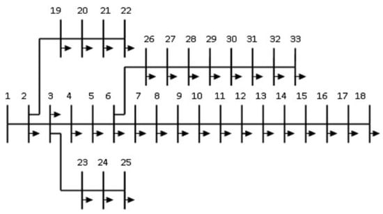
Figure 6.
Radial distribution system of IEEE 33-bus [35].
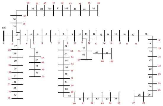
Figure 7.
Radial distribution system of IEEE 69-bus [33].
Usually, in a domestic household there are four types of loads present around the year that are considered in the analysis of a distribution system: electrical, heating, cooling and water heating loads. The peak values of these loads during the different periods of a year are listed in Table 2. It is observed that the heating load in the warming and moderate periods is zero, whereas the cooling load is zero in the cooling and moderate periods. The water heating and electrical loads are required in every period throughout the year.
Table 2.
Peak of four different load types (kW).
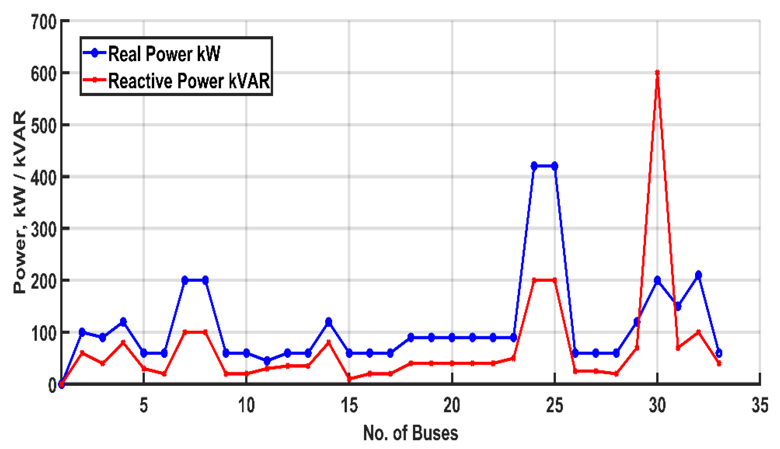
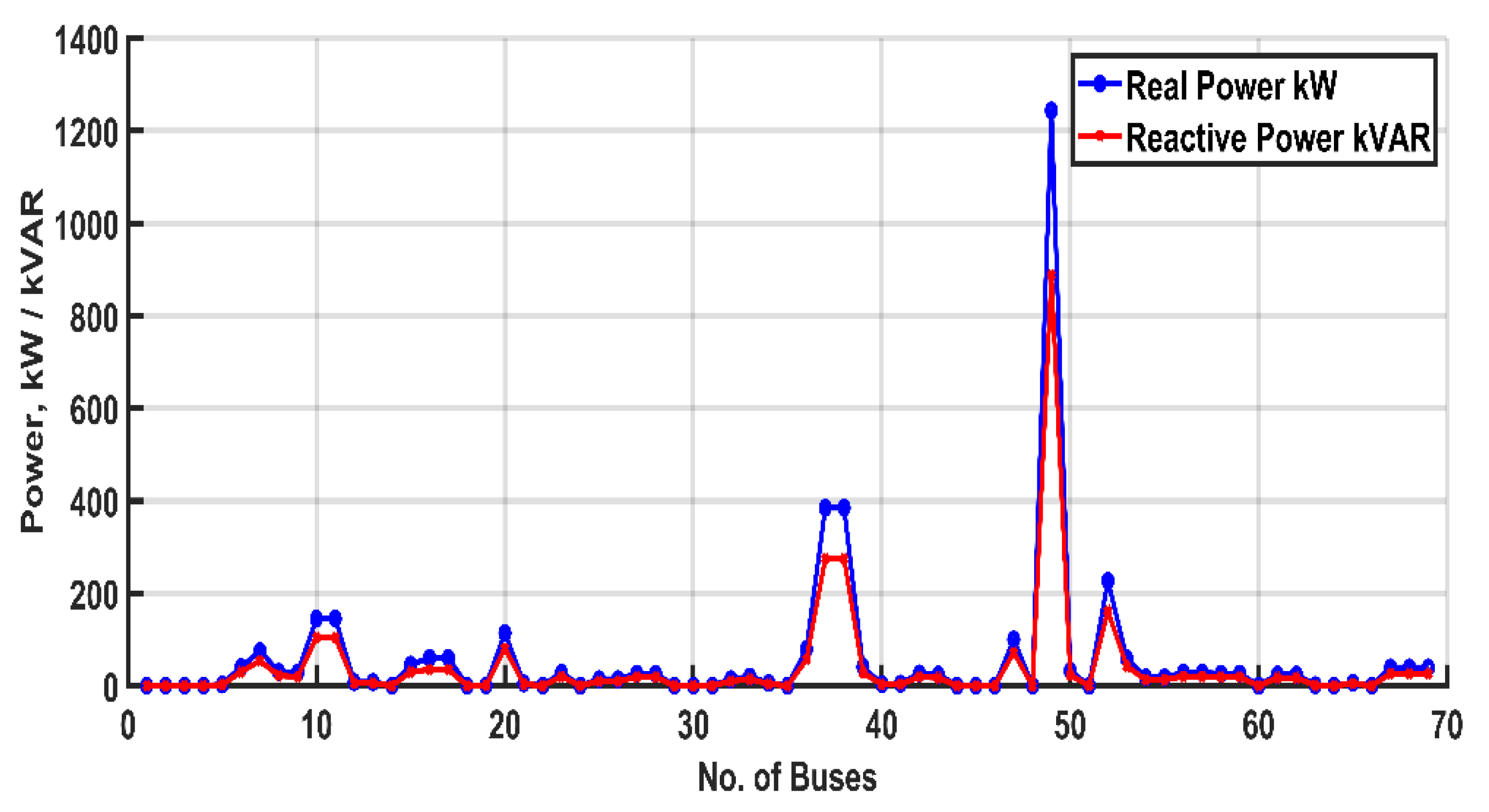
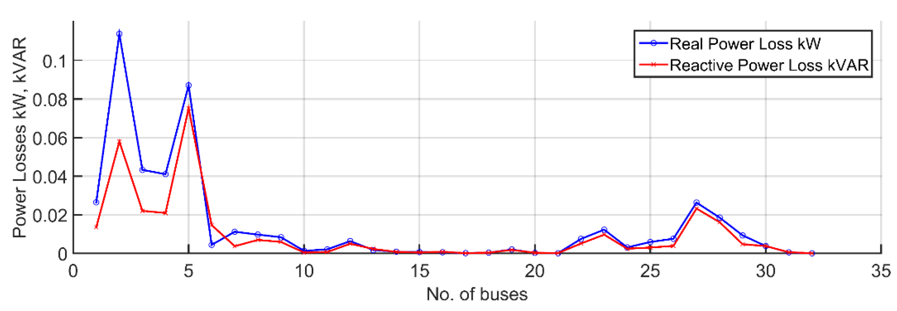
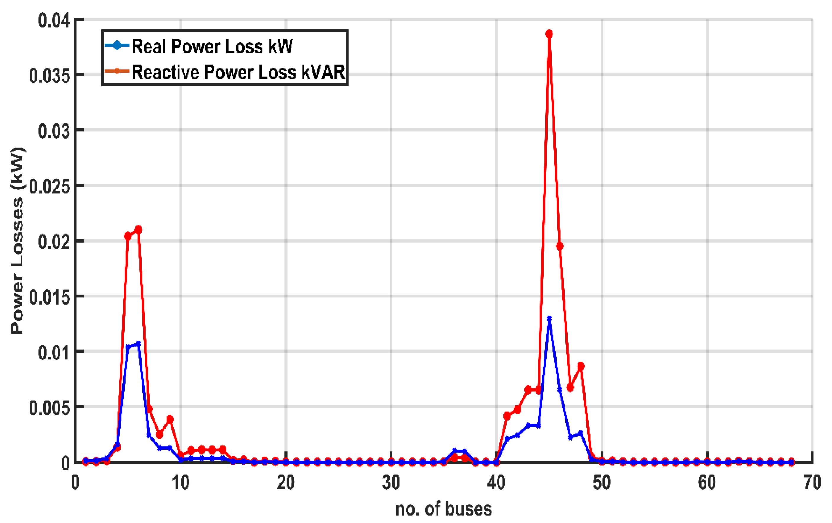
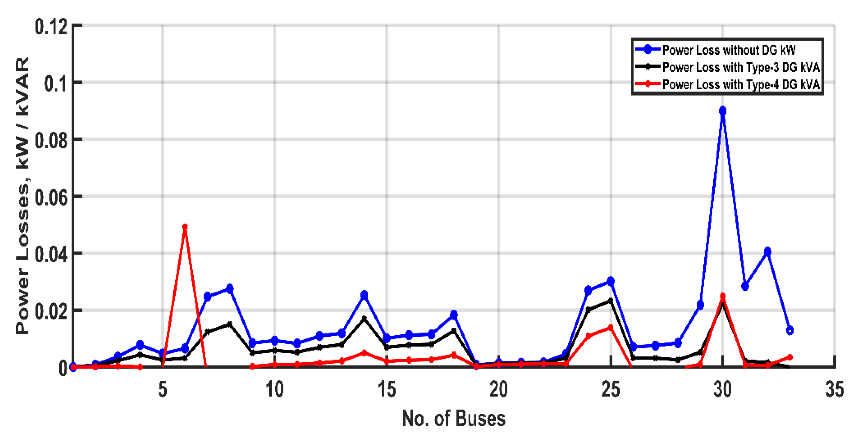
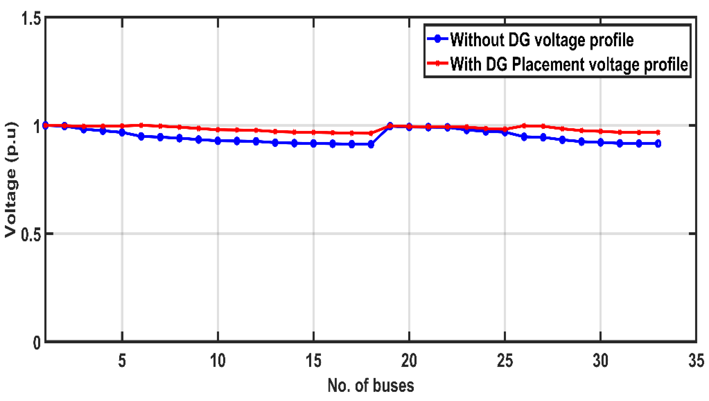
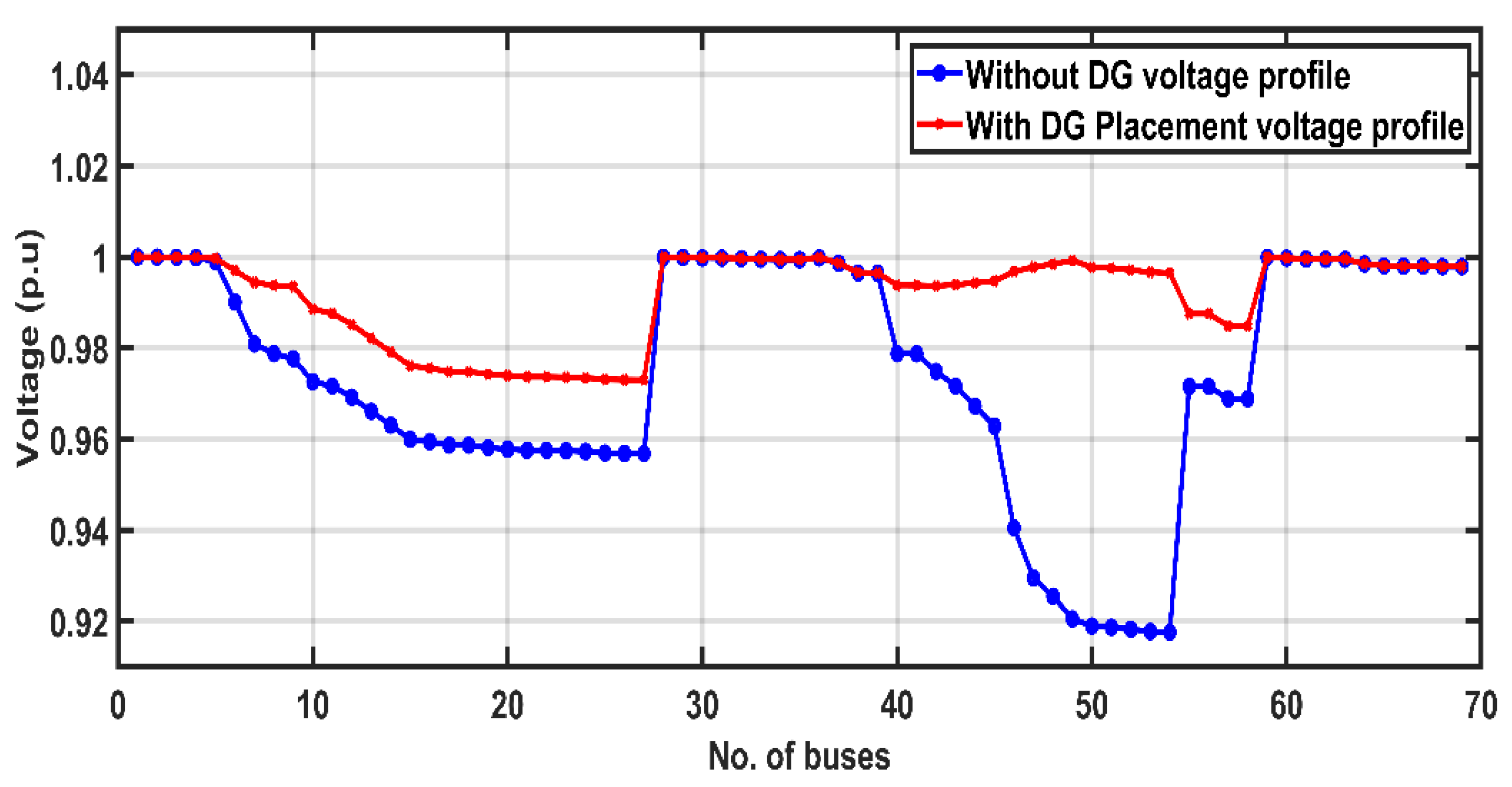
The contribution of the active and reactive power of a bus is dependent on the load profile of a bus. For an IEEE 33-bus system, the reactive power demand at bus 30 in Figure 8 reaches up to 600 kVAR and the active power demand is negligible, whereas for an IEEE 69-bus system at bus 50, the active and reactive power reaches 1250 kW and 900 kVAR in Figure 9. The active power losses (kW) in 33-bus and 69-bus systems without the allocation of DGs in the system are seen in Figure 10 and Figure 11 showing that the highest power loss is 0.11 kW at the 2nd bus and 0.013 kW at the 45th bus. After allocation of DG type-1 and type-3 at 0.9 and unity power factor, respectively, active and reactive power losses are detailed in Figure 12 and Figure 13. The maximum losses are 0.09 kW with the allocation of DG type-1 and minimum with the placement of type-3 DG at 0.9 pf lagging. Without the optimal allocation of any DG, the balance of power is not evenly distributed and there is room for improvement in the system. This challenge is resolved by either an even distribution of the load profile or by inserting optimal DGs into the system. The voltage variations per unit across 33-bus and 69-bus distribution power systems are represented in Figure 14 and Figure 15. It is observed that few buses have a voltage less than 0.95 (p.u) because of the power losses at these buses. These power losses may occur because of the impedance of the overall system or copper losses due to more current withdrawn by the buses as they have heavy loads attached to them.
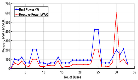
Figure 8.
Real and reactive power variations of 33-bus distribution system without DG placement.
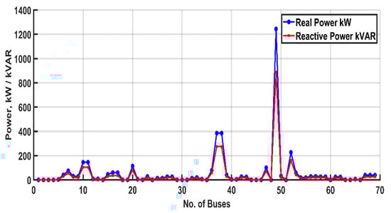
Figure 9.
Real and reactive power variations of 69-bus distribution system without DG placement.
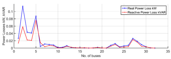
Figure 10.
Real and reactive power loss variation of 33-bus distribution system without any DG placement.
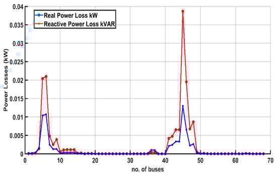
Figure 11.
Real and reactive power loss variation of 69-bus distribution system without any DG placement.
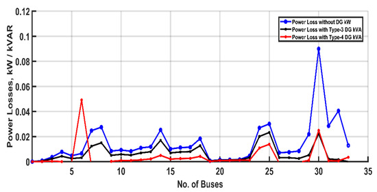
Figure 12.
Power loss variation of 33-bus distribution system after DG type-3 and type-4 placement.
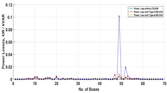
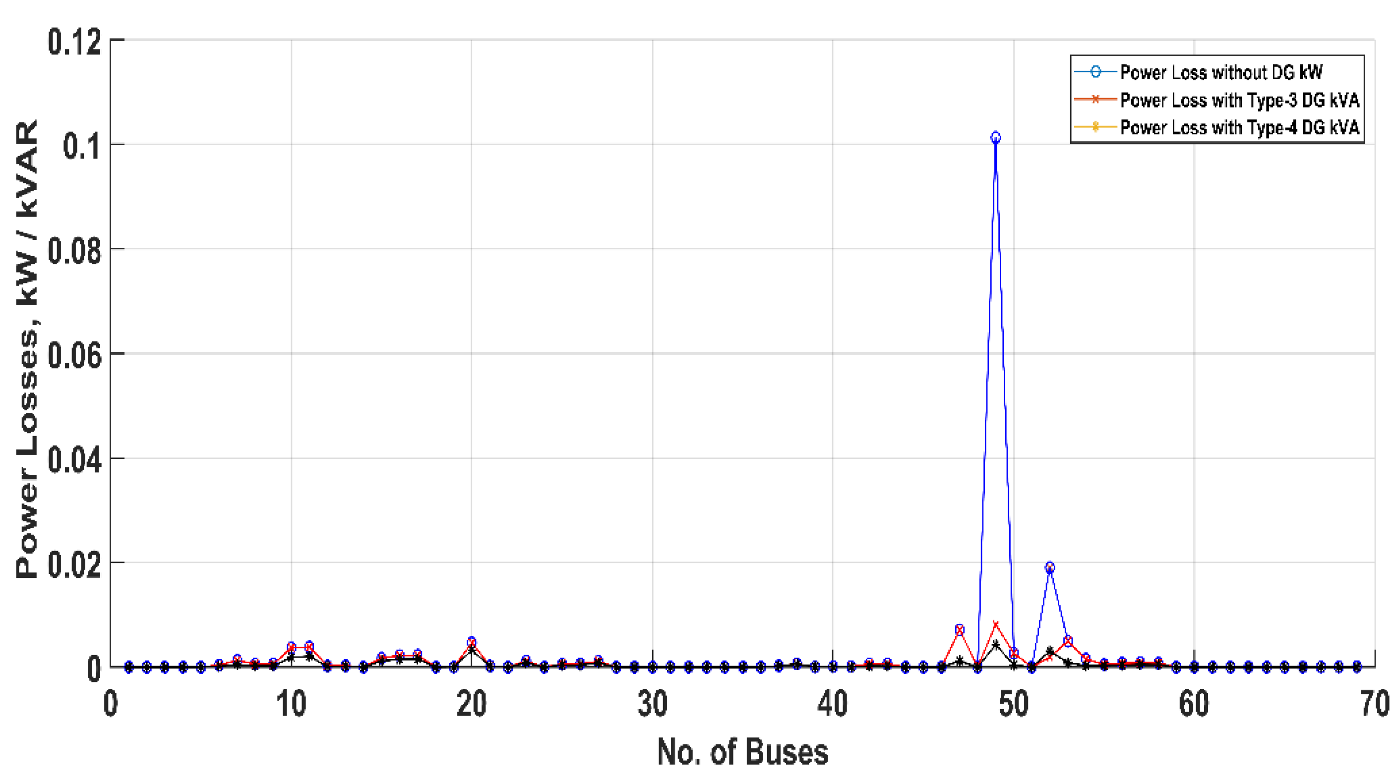
Figure 13.
Power loss variation of 69-bus distribution system after DG type-3 and type-4 placement.

Figure 14.
Voltage profile variation (p.u) of 33-bus distribution system before and after DG placement.
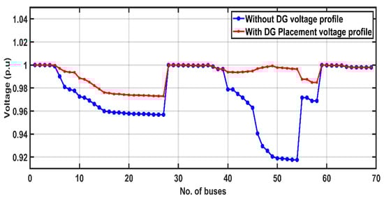
Figure 15.
Voltage profile variation (p.u) of 69-bus distribution system before and after DG placement.
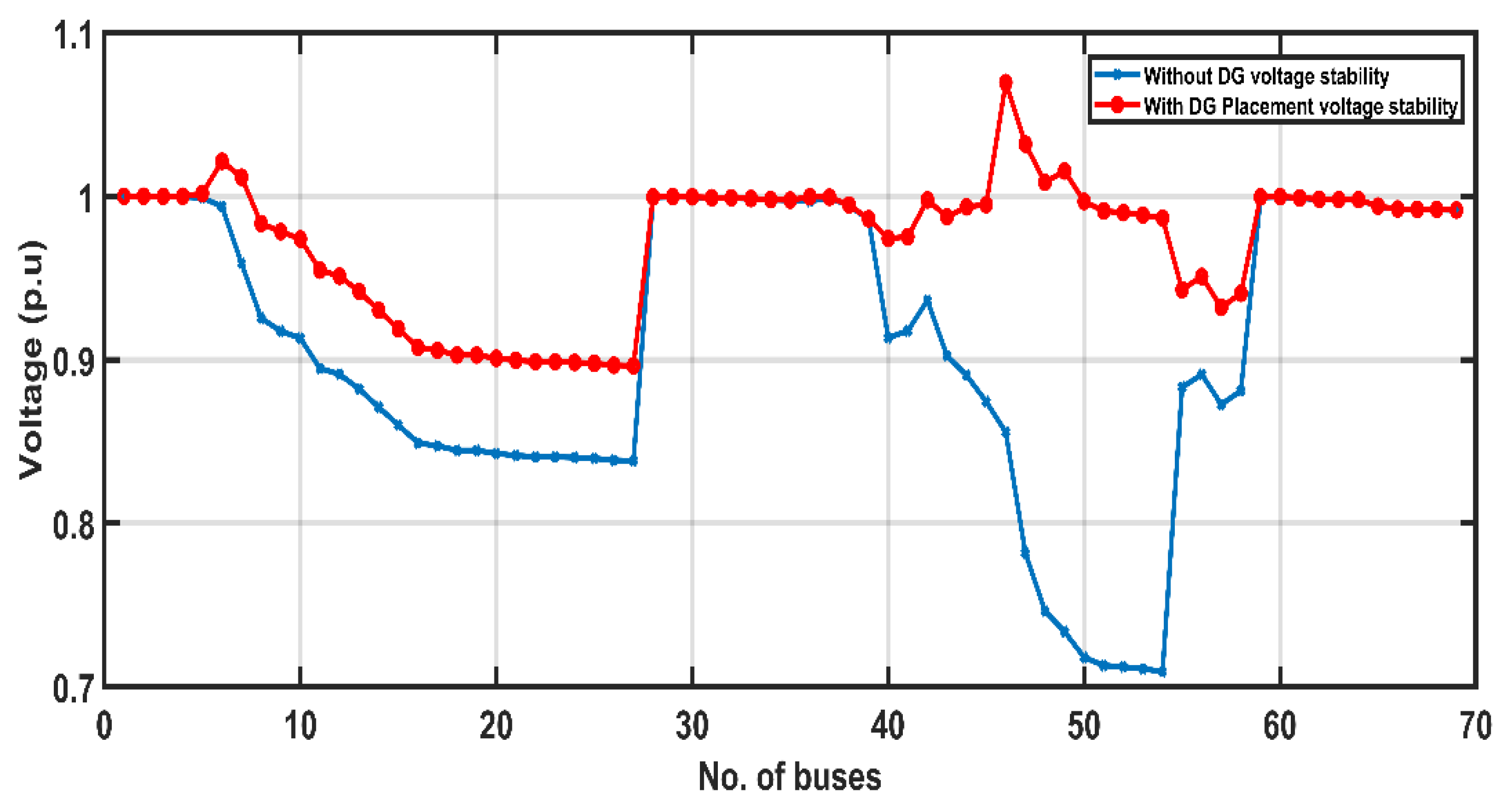
In this research work, four different types of DGs are used depending upon the ability of a DG to either provide or absorb active and reactive power in the system. Table 3 and Table 4 list the results regarding the active and reactive power loss, DG location and sizes in IEEE 33-bus and 69-bus systems for four different types of DGs. The optimal location of single DG placement by the PLI method is at the 30th bus for 33-bus systems and at the 61st bus for 69-bus systems in any of the four types of DG placement. The sizes of DGs are evaluated by optimizing the objective function using three metaheuristic optimization algorithms, i.e., HBA, GWO and WOA. The process of the whole optimization procedure is displayed in Figure 5. The overall voltage profile is boosted as we reduce the power losses by optimal allocation of the four DGs in the system. Voltage at each bus is within the bounds of the constraints and very near to the ideal value of 1 p.u. The improvements in the stability before and after allocation of the DGs are displayed in Figure 16 and Figure 17.
Table 3.
DG placement and its sizing data in a 33-bus distribution system.
Table 4.
DG placement and its sizing data in a 69-bus distribution system.
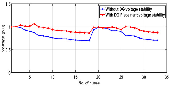
Figure 16.
Voltage stability variation (p.u) of 33-bus distribution system before and after DG placement.

Figure 17.
Voltage stability variation (p.u) of 69-bus distribution system before and after DG placement.
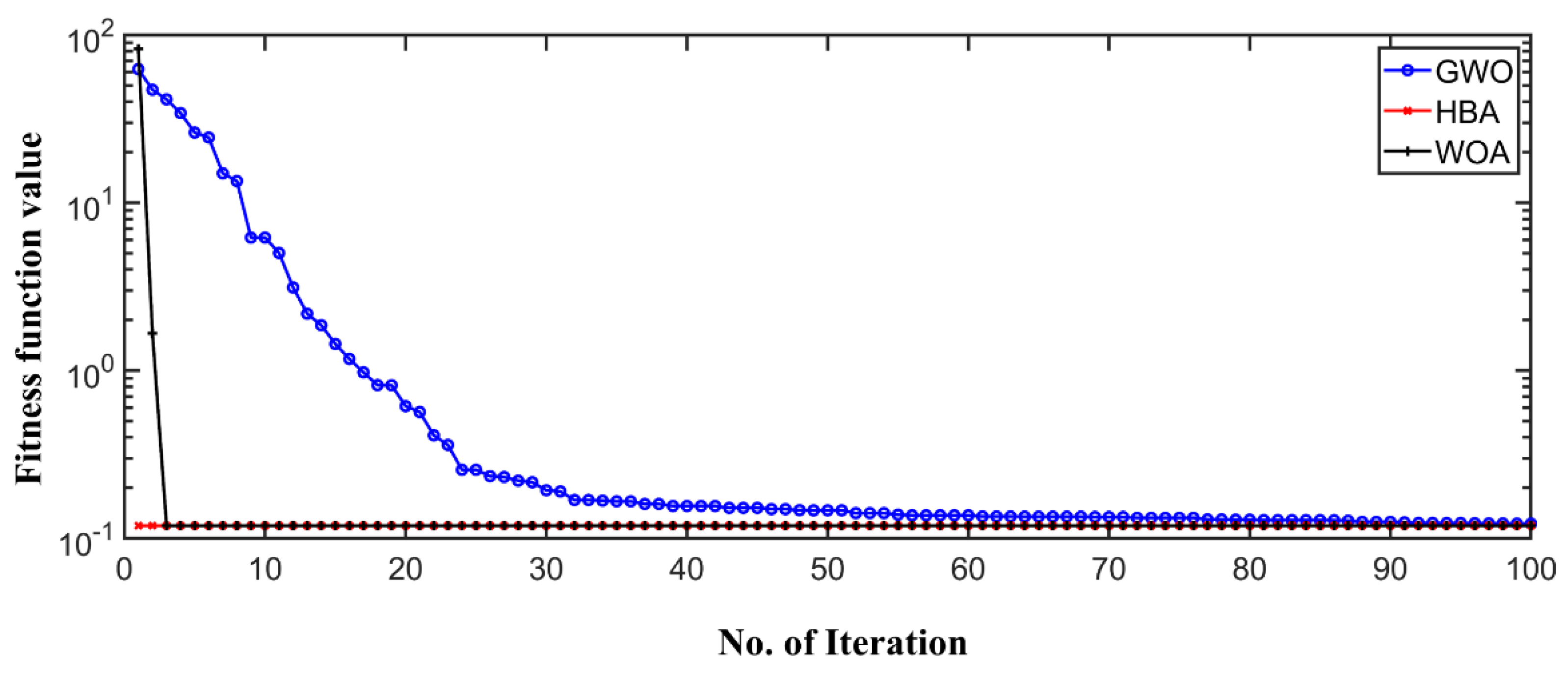
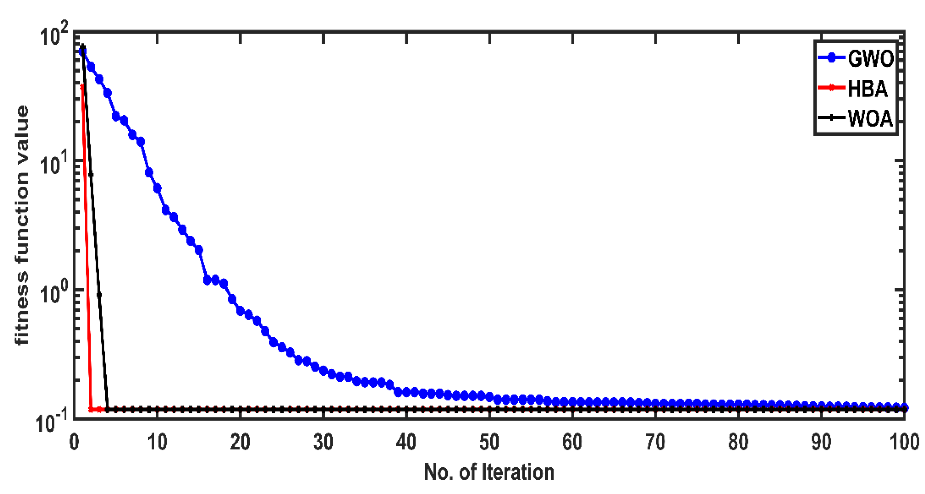
DG sizing is executed by applying three metaheuristic optimization algorithms. These algorithms converge in a specific time period depending upon the complexity, size of the problem and the searching ability of these algorithms. Almost every optimization algorithm tries to achieve the global best solution in a short time span to avoid divergence at any point. In Figure 18 and Figure 19, it is noticed that HBA took one and two iterations for IEEE 33-bus and 69-bus, respectively, to achieve the optimum and accurate results, far faster than WOA which converged in three iterations. GWO achieved its best possible solution in a higher number of iterations. The convergence curves of the implimented optimization algorithms are as follows:
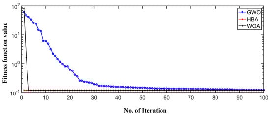
Figure 18.
Comparison of convergence curves for three metaheuristic algorithms in a 33-bus distribution system.
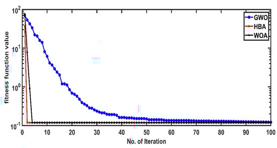
Figure 19.
Comparison of convergence curves for three metaheuristic algorithms in a 69-bus distribution system.
The power losses in the system impose an overall cost which can be calculated using Equation (38) [36].
where is the power tariff which has a value of 10.20 and is set by the power regulatory authority. All the costs of the DG power losses (CPL) are calculated and listed in Table 5. The least power loss cost is for type-2 and type-4 DGs in IEEE 33-bus and 69-bus systems, respectively, and the maximum cost of power losses is without DG placement.
Table 5.
Cost of power losses (CPL) in the distribution system.
7. Conclusions
In this paper, honey badger algorithm (HBA) was used to size the DGs optimally in IEEE 33-bus and 69-bus power distribution test bench systems to boost the overall voltage profile and stability by minimizing the power losses in a system, while a comparison was drawn with whale optimization algorithm (WOA) and grey wolf optimization (GWO). Four types of DGs were used during the whole optimization process. These algorithms were deployed to find the optimum DG values from the combination of random DG population. The results of the simulation authenticate that the power losses are reduced substantially, and voltage profile and stability improvement is observed, using a specially designed objective function. Also, the results point us to the fact that HBA was far faster than GWO and WOA, reaching the optimum solution in a mere one and two iterations for IEEE 33-bus and 69-bus, respectively, whereas WOA took three iterations. HBA has the strong capability to attain the best solution in a short number of iterations with higher accuracy than the other algorithms. In future work, we will extend our technique, which is designed to optimize DG sizing and allocation in low-voltage power distribution systems, to complex optimization problems in power distribution systems, i.e., the IEEE 8500 test system and the test circuits made available by the Electric Power Research Institute (EPRI), due to its robustness, accuracy and ability to reach optimal results in fewer iterations.
Author Contributions
Conceptualization, M.H.K. and A.U.; Funding acquisition, N.U.; Investigation, M.H.K.; Methodology, M.H.K.; Project administration, A.U.; Resources, A.U., A.K. and N.U.; Software, A.U. and H.S.Z.; Supervision, A.U.; Validation, M.H.K., A.K. and N.U.; Visualization, M.H.K., A.U., H.S.Z., M.A. and A.A.A.; Writing—original draft, M.H.K.; Writing—review & editing, A.U., A.K., H.S.Z., M.A., A.A.A. and N.U. All authors have read and agreed to the published version of the manuscript.
Funding
This research work was supported by the Taif University Researchers Supporting Project (TURSP-2020/144), Taif University, Taif, Saudi Arabia.
Institutional Review Board Statement
Not applicable.
Informed Consent Statement
Not applicable.
Data Availability Statement
Not applicable.
Conflicts of Interest
The authors declare no conflict of interest.
References
- Lee, S.H.; Grainger, J.J. Optimum Placement of Fixed and Switched Capacitors on Primary Distribution Feeders. IEEE Trans. Power Appar. Syst. 1981, 100, 345–352. [Google Scholar] [CrossRef]
- Hussain, I.; Khan, F.; Ahmad, I.; Khan, S.; Saeed, M. Power Loss Reduction via Distributed Generation System Injected in a Radial Feeder. Mehran Univ. Res. J. Eng. Technol. 2021, 40, 160–168. [Google Scholar] [CrossRef]
- Bollen, M.; Yang, Y.; Hassan, F. Integration of distributed generation in the power system-a power quality approach. In Proceedings of the 13th International Conference on Harmonics and Quality of Power IEEE, Wollongong, NSW, Australia, 28 September–1 October 2008; pp. 1–8. [Google Scholar] [CrossRef]
- Devabalaji, K.; Ravi, K.; Kothari, D. Optimal location and sizing of capacitor placement in radial distribution system using Bacterial Foraging Optimization Algorithm. Int. J. Electr. Power Energy Syst. 2015, 71, 383–390. [Google Scholar] [CrossRef]
- Franco, J.F.; Rider, M.J.; Lavorato, M.; Romero, R. A mixed-integer LP model for the optimal allocation of voltage regulators and capacitors in radial distribution systems. Int. J. Electr. Power Energy Syst. 2013, 48, 123–130. [Google Scholar] [CrossRef]
- Reddy, P.D.P.; Reddy, V.C.V.; Manohar, T.G. Whale optimization algorithm for optimal sizing of renewable resources for loss reduction in distribution systems. Renew. Wind. Water Sol. 2017, 4, 3. [Google Scholar] [CrossRef]
- Hung, D.Q.; Mithulananthan, N.; Bansal, R.C. Analytical Expressions for DG Allocation in Primary Distribution Networks. IEEE Trans. Energy Convers. 2010, 25, 814–820. [Google Scholar] [CrossRef]
- Golberg, D.E. Genetic Algorithms in Search, Optimization, and Machine Learning. Available online: http://www2.fiit.stuba.sk/~kvasnicka/Free%20books/Goldberg_Genetic_Algorithms_in_Search.pdf (accessed on 6 July 2022).
- Kennedy, J.; Eberhart, R. Particle Swarm Optimization. In Proceedings of the ICNN’95—International Conference on Neural Networks, Perth, Australia, 27 November–1 December 1995; Volume 4, pp. 1942–1948. [Google Scholar] [CrossRef]
- Sultana, U.; Khairuddin, A.B.; Rasheed, N.; Qazi, S.H.; Mokhtar, A.S. Allocation of Distributed Generation and Battery Switching Stations for Electric Vehicle using Whale Optimiser Algorithm. J. Eng. Res. 2018, 6, 70–93. [Google Scholar]
- Suresh, M.C.V.; Belwin, E.J. Optimal DG placement for benefit maximization in distribution networks by using Dragonfly algorithm. Renew. Wind. Water Sol. 2018, 5, 4. [Google Scholar] [CrossRef]
- Tan, Z.; Zeng, M.; Sun, L. Optimal Placement and Sizing of Distributed Generators Based on Swarm Moth Flame Optimization. Front. Energy Res. 2021, 9, 676305. [Google Scholar] [CrossRef]
- Anbuchandran, S.; Rengaraj, R.; Bhuvanesh, A.; Karuppasamypandiyan, M. A Multi-objective Optimum Distributed Generation Placement Using Firefly Algorithm. J. Electr. Eng. Technol. 2021, 17, 945–953. [Google Scholar] [CrossRef]
- Nekooei, K.; Farsangi, M.M.; Nezamabadi-Pour, H.; Lee, K.Y. An Improved Multi-Objective Harmony Search for Optimal Placement of DGs in Distribution Systems. IEEE Trans. Smart Grid 2013, 4, 557–567. [Google Scholar] [CrossRef]
- Aman, M.M.; Jasmon, G.B.; Mokhlis, H.; Abu Bakar, A.H. Optimum tie switches allocation and DG placement based on maximisation of system loadability using discrete artificial bee colony algorithm. IET Gener. Transm. Distrib. 2016, 10, 2277–2284. [Google Scholar] [CrossRef]
- Mirjalili, S.; Lewis, A. Advances in Engineering Software the Whale Optimization Algorithm. Adv. Eng. Softw. 2016, 95, 51–67. [Google Scholar] [CrossRef]
- Mirjalili, S.; Mirjalili, S.M.; Lewis, A. Advances in Engineering Software Grey Wolf Optimizer. Adv. Eng. Softw. 2014, 69, 46–61. [Google Scholar] [CrossRef]
- Hashim, F.A.; Houssein, E.H.; Hussain, K.; Mabrouk, M.S.; Al-Atabany, W. Honey Badger Algorithm: New metaheuristic algorithm for solving optimization problems. Math. Comput. Simul. 2022, 192, 84–110. [Google Scholar] [CrossRef]
- Abdel-Mawgoud, H.; Ali, A.; Kamel, S.; Rahmann, C.; Abdel-Moamen, M. A Modified Manta Ray Foraging Optimizer for Planning Inverter-Based Photovoltaic with Battery Energy Storage System and Wind Turbine in Distribution Networks. IEEE Access 2021, 9, 91062–91079. [Google Scholar] [CrossRef]
- Das, B.; Mukherjee, V.; Das, D. DG placement in radial distribution network by symbiotic organisms search algorithm for real power loss minimization. Appl. Soft Comput. 2016, 49, 920–936. [Google Scholar] [CrossRef]
- Saddique, M.W.; Haroon, S.S.; Amin, S.; Bhatti, A.R.; Sajjad, I.A.; Liaqat, R. Optimal Placement and Sizing of Shunt Capacitors in Radial Distribution System Using Polar Bear Optimization Algorithm. Arab. J. Sci. Eng. 2021, 46, 873–899. [Google Scholar] [CrossRef]
- Moradi, M.H.; Abedini, M. A combination of genetic algorithm and particle swarm optimization for optimal DG location and sizing in distribution systems. Int. J. Electr. Power Energy Syst. 2012, 34, 66–74. [Google Scholar] [CrossRef]
- Celli, G.; Ghiani, E.; Mocci, S.; Pilo, F. A Multiobjective Evolutionary Algorithm for the Sizing and Siting of Distributed Generation. IEEE Trans. Power Syst. 2005, 20, 750–757. [Google Scholar] [CrossRef]
- Gomez-Gonzalez, M.; López, A.; Jurado, F. Optimization of distributed generation systems using a new discrete PSO and OPF. Electr. Power Syst. Res. 2012, 84, 174–180. [Google Scholar] [CrossRef]
- Abdel-Mawgoud, H.; Kamel, S.; El-Ela, A.A.A.; Jurado, F. Optimal Allocation of DG and Capacitor in Distribution Networks Using a Novel Hybrid MFO-SCA Method. Electr. Power Components Syst. 2021, 49, 259–275. [Google Scholar] [CrossRef]
- De Koster, O.A.C.; Domínguez-Navarro, J.A. Multi-Objective Tabu Search for the Location and Sizing of Multiple Types of FACTS and DG in Electrical Networks. Energies 2020, 13, 2722. [Google Scholar] [CrossRef]
- Wang, C.; Nehrir, M. Analytical Approaches for Optimal Placement of Distributed Generation Sources in Power Systems. IEEE Trans. Power Syst. 2004, 19, 2068–2076. [Google Scholar] [CrossRef]
- Acharya, N.; Mahat, P.; Mithulananthan, N. An analytical approach for DG allocation in primary distribution network. Int. J. Electr. Power Energy Syst. 2006, 28, 669–678. [Google Scholar] [CrossRef]
- Keane, A.; O’Malley, M. Optimal allocation of embedded generation on the Irish distribution network. In Proceedings of the CIRED 18th International Conference and Exhibition on Electricity Distribution IET, Turin, Italy, 6–9 June 2005. [Google Scholar] [CrossRef]
- El-Fergany, A. Optimal allocation of multi-type distributed generators using backtracking search optimization algorithm. Int. J. Electr. Power Energy Syst. 2015, 64, 1197–1205. [Google Scholar] [CrossRef]
- Singh, B.; Mukherjee, V.; Tiwari, P. A survey on impact assessment of DG and FACTS controllers in power systems. Renew. Sustain. Energy Rev. 2015, 42, 846–882. [Google Scholar] [CrossRef]
- Kawambwa, S.; Mwifunyi, R.; Mnyanghwalo, D.; Hamisi, N.; Kalinga, E.; Mvungi, N. An improved backward/forward sweep power flow method based on network tree depth for radial distribution systems. J. Electr. Syst. Inf. Technol. 2021, 8, 7. [Google Scholar] [CrossRef]
- Reddy, P.D.P.; Reddy, V.C.V.; Manohar, T.G. Optimal renewable resources placement in distribution networks by combined power loss index and whale optimization algorithms. J. Electr. Syst. Inf. Technol. 2018, 5, 175–191. [Google Scholar] [CrossRef]
- Ehsan, A.; Yang, Q. Optimal integration and planning of renewable distributed generation in the power distribution networks: A review of analytical techniques. Appl. Energy 2020, 210, 44–59. [Google Scholar] [CrossRef]
- Meera, P.S.; Hemamalini, S. Optimal Siting of Distributed Generators in a Distribution Network using Artificial Immune System. Int. J. Electr. Comput. Eng. 2017, 7, 641–649. [Google Scholar] [CrossRef]
- Kien, L.C.; Nguyen, T.T.; Pham, T.D.; Nguyen, T.T. Cost reduction for energy loss and capacitor investment in radial distribution networks applying novel algorithms. Neural Comput. Appl. 2021, 33, 15495–15522. [Google Scholar] [CrossRef]


Publisher’s Note: MDPI stays neutral with regard to jurisdictional claims in published maps and institutional affiliations. |
© 2022 by the authors. Licensee MDPI, Basel, Switzerland. This article is an open access article distributed under the terms and conditions of the Creative Commons Attribution (CC BY) license (https://creativecommons.org/licenses/by/4.0/).