Capability for Hydrogeochemical Modelling within Discrete Fracture Networks

Abstract

A new method for simulating solute transport and geochemical interactions within fractured rock is presented. This will be an important capability for assessing the safety of radioactive waste disposal facilities that are located within fractured crystalline bedrock. Specifically, the discrete fracture network (DFN) module within the ConnectFlow groundwater flow and transport software has been updated to: (i) simulate the advection and diffusion of more than one solute species (with the flow and transport equations coupled by the evolving density and viscosity); (ii) model the diffusion of solutes into the rock matrix between fractures; and (iii) utilise the iPhreeqc library to model chemical reactions involving solutes, minerals on fracture/pore surfaces and rock minerals. The performance of ConnectFlow’s DFN module has also been significantly improved via parallelisation which allows more complex calculations to be attempted. These developments are significant because hydrogeochemistry within fractured rock is more accurately represented in an explicit DFN, rather than using more approximate equivalent continuous porous medium (ECPM) methods. Illustrative calculations have been completed for the disposal facility for spent nuclear fuel at Olkiluoto in Finland, and the former candidate site for spent fuel disposal, Laxemar, in Sweden. These calculations show that DFN simulations provide results that are qualitatively similar to results from ECPM calculations. However, because the ECPM is a less direct approach, notable differences exist when compared to the DFN approach.

1. Introduction

The chemical composition of groundwater is a key consideration for the safety of geological radioactive waste disposal facilities [1,2,3]. For example, the hydrogeochemical evolution of the groundwater affects the stability of buffer materials that surround spent fuel canisters and the resilience of the spent fuel disposal canisters themselves. Two of the most advanced geological disposal programs are located at Forsmark in Sweden and Olkiluoto in Finland. Both disposal facilities will be located within fractured rock. This work presents a new capability for simulating hydrogeochemical evolution within fractured rock using a discrete fracture network (DFN). This allows the geometry, permeability and dispersion within the fracture network to be explicitly represented and removes some of the approximations inherent in other methods (such as ECPMS). Previous work [4] implemented reactive transport in Equivalent Continuous Porous Media (ECPM) models. ECPMs use an upscaling approximation to transfer the properties of fractures onto a three-dimensional mesh; the groundwater flow, transport and reaction equations are then solved on this mesh. The upscaling approximation does have limitations; for example, it can produce additional unphysical connectivity [5] and it can be difficult to determine an appropriate upscaled porosity.

In the discrete fracture network (DFN) method described here, the ECPM approximations are not needed. Each fracture is discretised using a two-dimensional mesh; the flow, transport and reaction equations are solved on an intersecting network of these two-dimensional meshes. Efficient algorithms are utilised that allow large fracture networks to be simulated.

Until recently, most previous attempts to model reactive transport in fractured rock have relied on an ECPM approach or have used an explicit DFN discretisation for a relatively small number of fractures. For example, a micron-scale structured grid is used in [6] to represent their DFN and focus on the immediate surroundings of a deposition hole for a radioactive waste canister. Similarly, in [7], reactive transport modelling is considered in the area immediately surrounding a canister in a deposition hole, and in [8], an equivalent porous medium representation is created for the vitrified fractured glass block used to encase the high-level nuclear waste within a deposition hole. All these studies aim to model a deposition hole and its contents in detail, which is a somewhat different goal to the modelling of an entire disposal facility or a wider site. A deposition hole is not explicitly considered in [9]; instead, an ECPM is used to consider in detail the small crystalline grains within a sample that has a volume of 1 cm³.

There are other models that aim to model larger volumes, though these tend to simplify the system. Transport is simulated in a DFN-based model using random-walk particle tracking [10], which is then used as a basis for calculating reactive transport. However, these calculations are performed on a single fracture or in a two-dimensional fracture network. A reactive transport model of the Forsmark site is presented in [11], the selected location for spent fuel disposal in Sweden, using an ECPM representation of the DFN. An analytical method and an ECPM representation are used in [12] to simulate the future evolution of groundwater salinity within the repository at Olkiluoto. The analytical models attempt to apply retardation and dispersion to the results of particle tracking, although these models do not couple the transport and flow equations.

A chemical reaction between two solute plumes is modelled in [13] for a three-dimensional fracture network containing a moderate number of fractures. This has similarities with the method presented here. The single generic reaction considered is naturally much simpler than the range of chemical reactions that might be included for a real disposal facility. From a different perspective, a specific reaction is modelled in [14] using PHREEQC in a discrete fracture network model; however, their calculations are based on hydrolysis reactions within the groundwater and do not consider the effects of reactions between solutes and either the rock matrix or other solutes.

The methods developed here have been applied to illustrative site-scale models (spanning several cubic kilometres) of the spent nuclear fuel repository at Olkiluoto in Finland and the former candidate site at Laxemar site in Sweden. These models include tens of thousands of fractures and represent a major advance in reactive transport modelling capability for fractured rock geologies.

2. Materials and Methods

2.1. Equations for Solute Transport within DFNs

The equations below (based on [15]) can be used to represent Darcy flow, and the transport of n solutes $c_i=c_1, c_2, \dots , c_n$ through a single fracture. The diffusion of solutes into the surrounding rock matrix [15] is explicitly included (known as rock matrix diffusion or RMD), while unsaturated groundwater flow and heat transport are not considered.

$$\frac{\partial }{\partial t}\left[e_t\rho \left(c_i,P_R\right) \right]+\overrightarrow{\nabla }·[\rho \left(c_i,P_R\right)\overrightarrow{Q}]=0$$

(1)

$$\frac{\partial }{\partial t}\left[e_t\rho \left(c_i,P_R\right)c_i\right]+\overrightarrow{\nabla }·[\rho \left(c_i,P_R\right)\overrightarrow{Q}{c}_i]=\overrightarrow{\nabla }·[e_t\rho \left(c_i,P_R\right)D·\overrightarrow{\nabla }{c}_i]+2\rho \left(c_i,P_R\right)D_i{\frac{\partial c_i^{\prime }}{\partial w}|}_{w=0}$$

(2)

$$\overrightarrow{Q}=\frac{e_h^3}{12\mu \left(c_i,P_R\right) }[\overrightarrow{\nabla }{P}_R-\left(\rho \left(c_i,P_R\right)-{\rho }_0\right)g\overrightarrow{z}]$$

(3)

$$\alpha \frac{\partial }{\partial t}\left[\rho \left(c_i,P_R\right)c_i^{\prime }\right]=\frac{\partial }{\partial w}[D_i\rho \left(c_i,P_R\right)\frac{\partial \rho \left(c_i\prime ,P_R\right)c_i^{\prime }}{\partial w}]$$

(4)

Here, $n$ versions of Equations (2) and (4) are required to model the transport of $n$ solutes. Equation (4) is usually simplified by assuming constant density within the matrix. The variables referred to are:

• $P_R$ [Pa] the residual pressure: $P_R=P_T+{\rho }_{0}gz;$ (where g is the acceleration due to gravity, $z$ is the elevation above sea level, $P_T$ is the total pressure and ${\rho }_0$ is a reference density);
• $c_i$ [-] the mass fraction of solutes in the fracture;
• $c_i^{\prime }$ [-] the mass fraction of solutes in the matrix;
• $e_h$ [m] the effective hydraulic aperture in the fracture;
• $e_t$ [m] the transport aperture in the fracture;
• $\rho \left(c_i,P_R\right)$ [kg m⁻³] and $\mu \left(c_i,P_R\right)$ [kg m⁻¹ s⁻¹] the fluid density and viscosity, respectively. These can be calculated using an empirical expression [16];
• $\overrightarrow{Q}$ [m² s⁻¹] the volume of water flowing per second, per unit width of the fracture;
• $t$ [s] the time;
• $\overrightarrow{\nabla }$ the two-dimensional gradient operator within the fracture;
• $D$ [m² s⁻¹] the dispersion tensor within the mobile water in the fracture; this includes contributions from diffusion and from hydrodynamic dispersion; the latter has components parallel and perpendicular to the flow;
• $D_i$ [m² s⁻¹] the intrinsic diffusion coefficient for diffusion into the rock matrix;
• $w$ [m] the perpendicular distance from the fracture plane into the rock matrix;
• $\alpha$ [-] the capacity factor (when there is no sorption, this is the same as the porosity of the matrix).

These equations are analogous to those for a Continuous Porous Medium (CPM) described in [4]. The viscosity and density are dependent on the solute concentrations, and hence couple together the groundwater flow and transport equations. These equations have been implemented explicitly for discrete fracture networks within ConnectFlow’s DFN module, as described in [17]. More details of the implementation are included in the following subsections.

Equations (1) to (4) do not include chemical reactions. Reactions, involving solutes and rock minerals, within the fracture porewater and the rock matrix, have also been implemented for DFNs in ConnectFlow. This capability is described further in Section 2.5.

2.2. DFNs in ConnectFlow

The ConnectFlow software [17] is a finite-element package for simulating the migration of fluids and solutes through fractured and porous rocks. The approach for modelling groundwater flow in DFNs in ConnectFlow is simple and very efficient. The algorithms divide the calculation into stages (Figure 1); several groundwater flow calculations are carried out on each fracture, with each calculation determining one of the global basis functions for that fracture (see below); next, the flow in the overall network is obtained using these global basis functions on each fracture together with the conditions that:

• The groundwater pressures are continuous between two intersecting fractures.
• Groundwater fluxes are conserved at an intersection between fractures.

When modelling solute transport, a very similar process is followed, with equivalent constraints for continuity and flux balance enforced for each solute.

The DFN module of ConnectFlow uses a Galerkin [18] finite-element approach. This method is used on two levels: for each individual fracture and for the whole network along fracture intersections. In the Galerkin method, the nodal mass fluxes are conserved, but mass is not conserved locally (this can be an issue for particle tracking calculations, which is rectified using a post-processing step [19]).

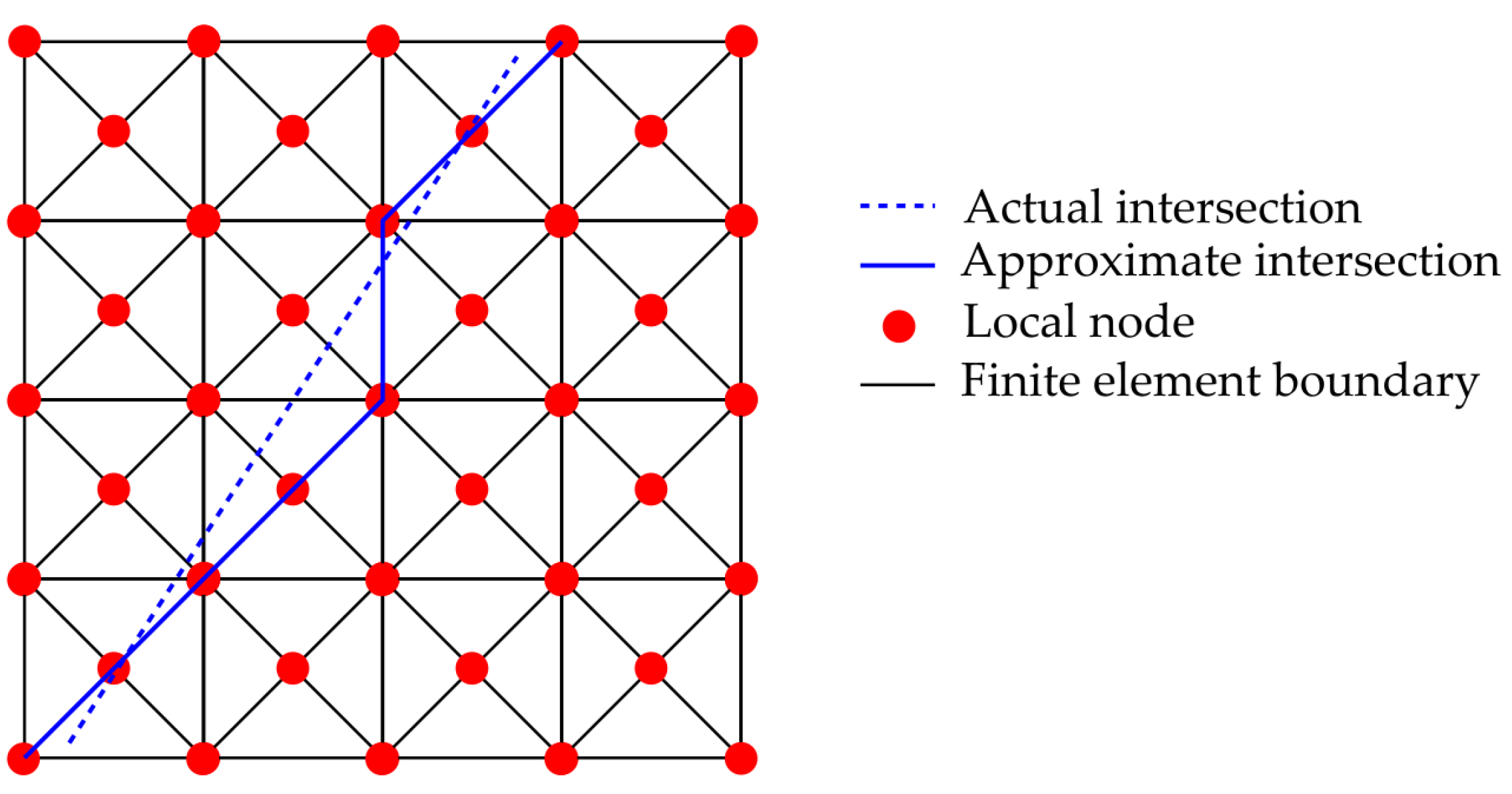
• A regular mesh of triangular elements is used to discretise individual fractures, as shown in Figure 2. The pressure and concentration are approximated on each element as a linear combination of basis functions. For each element, there is an associated node. For example, the pressure is given by

  $$P(\overrightarrow{x})={\displaystyle \sum }_i{\varphi }_i(\overrightarrow{x})P_i$$

  (5)
  where $P_i$ is the pressure at node i, and the basis function ${\varphi }_i,$ associated with node i, takes the value 1 at the node and 0 at all the other nodes. These nodes are referred to as “local nodes” in ConnectFlow.
  Each triangular finite element on the fracture can have a different hydraulic aperture, with values typically sampled from a probability distribution function.
• For the overall fracture network, the pressure and concentration are defined by their values at “global nodes” that exist on the intersections between fractures. The intersections are approximated using the lines formed by the boundaries of the triangular elements on the fracture (see Figure 2). The global nodes coincide with local nodes on the approximated intersection. The global problem does not have a separate mesh but rather relies on the underlying mesh on each fracture.
  Each global node I has a corresponding global basis function. This global basis function is approximated by the finite-element solution for the steady-state groundwater flow equations on the fracture in the case in which the residual pressure is specified to be $1$ at global node $I$ and $0$ at all the other global nodes on the fracture. The global flow and transport calculations can either be steady state or fully transient.

The global basis functions are then used to assemble the global finite element equations which are then solved. The use of basis functions, calculated from the groundwater flow equations to model solute transport, is an approximation that saves significant computational effort. However, the salinity distribution on a fracture is determined using functions with a fairly low number of degrees of freedom (equal to the number of global nodes on intersections rather than the number of local nodes). This method is therefore not expected to represent large variations of salinity within a single fracture. Where fractures are big enough that the salinity varies significantly within them, they can be tessellated into smaller sub-fractures, so that the salinity variation is relatively small within each tessellate. This means the fracture tessellation length should be smaller than the longitudinal dispersion length. A fuller description of the ConnectFlow algorithms is provided in [17].

Simulations of reactive transport for multiple species are challenging notwithstanding the efficiency of the algorithms described above. Therefore, every attempt has been made to enhance the performance via parallelisation and efficient algorithms. As noted in Figure 1, the first step of each calculation is performed on each fracture separately. Consequently, this can be easily parallelised, with each CPU core processing a different group of fractures, with minimal communication between cores. Conveniently, this step is also the slowest and gains the most performance benefit from parallelisation. ConnectFlow uses the distributed memory Message Parsing Interface (MPI) for parallelisation.

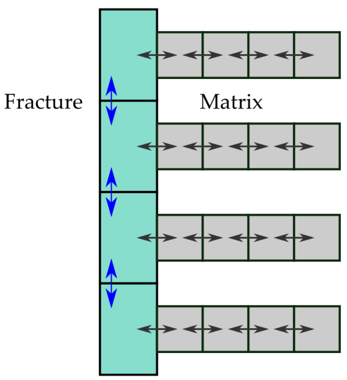
2.3. Rock Matrix Diffusion

Solutes can diffuse from flowing water within the fractures into the immobile water in the adjacent rock matrix (given a gradient in the concentration) [20]. This process is known as rock matrix diffusion, or RMD, and retards the transport of solutes (assuming that the porewater in the matrix is immobile). The rock matrix may also be an important site for chemical reactions because there can be significant pore surface areas within the rock matrix.

A numerical scheme for determining the diffusive flux between the mobile porewater and the matrix, for an upscaled ECPM model, is presented in [4]. A similar approach is used here to represent the rock matrix in a DFN (see Figure 3). Using a one-dimensional finite volume discretisation, and assuming the fluid density in the matrix is constant, Equation (4) becomes

$$\frac{\alpha ({c^{\prime }}_j^n-c_j^{\prime n-1})}{\mathsf{\Delta }t}=\frac{2D_j}{\mathsf{\Delta }{w}_j}\left\{\frac{({c^{\prime }}_{j+1}^n-c_j^{\prime n})}{\mathsf{\Delta }{w}_j+\mathsf{\Delta }{w}_{j+1}}-\frac{({c^{\prime }}_j^n-{c^{\prime }}_{j-1}^n)}{\mathsf{\Delta }{w}_{j-1}+\mathsf{\Delta }{w}_j}\right\} .$$

(6)

The term in Equation (2) representing the diffusive flux $F$ (advection into the matrix is ignored) between the fracture and the surrounding matrix becomes

$$F=\frac{4\rho D_i}{\mathsf{\Delta }{w}_1}({c^{\prime }}_1^n-c_j^n)$$

(7)

where the index $j$ indicates the finite volume (note we have dropped the species index here), with index $j=1$ representing the volume adjacent to the fracture; and index $n$ indicates the time step. Following the derivation from [4], Equation (7) can be written in the following form:

$$F=A^n+B\frac{c^n-c^{n-1}}{t^n-t^{n-1} }$$

(8)

where $c^n$ is the concentration in the fracture system at the end of time step n, and the coefficients $A^n$ and B do not depend on $c^n$. Conveniently, $A^n$ and B are calculated from matrix concentrations at previous time steps. This means that the inclusion of rock matrix diffusion does not require the simultaneous calculation of the fracture and matrix concentrations, and significantly reduces the computational burden.

In ConnectFlow, fractures can be tessellated into smaller sub-fractures, which themselves consist of finite elements. Diffusion between fractures and the matrix are calculated at the centre of each sub-fracture. The number of sub-fractures within a fracture can be increased to better represent the diffusive flux between the fracture and the matrix. This can be important for accurately simulating a solute mixing front moving through the fracture network.

Rock matrix diffusion calculations are defined according to the following parameters:

• The total diffusion length into the matrix $w_{max}={\displaystyle \sum }_{j=1,n_{fv}}{w}_i\left[m\right]$;
• The number of finite volume cells per global node, $n_{fv}$;
• The intrinsic diffusion coefficient, $D_i$ [m²/s];
• The porosity of the matrix or capacity factor,$\alpha$ [-].

The total diffusion length into the rock matrix should be bounded by the half distance to the adjacent fractures. This is because diffusion of solutes can propagate through a matrix block from fractures on both sides. For non-parallel fractures, the shortest distance between the fractures will vary over the fracture surface, making it more difficult to specify a maximum diffusion length. This can be ameliorated by tessellating larger fractures, with each subfracture having its own diffusion length.

2.4. Representation of Solute Concentrations

Concentrations typically have one of two representations within ConnectFlow:

• As a mass fraction, c, of a solute species, i, calculated from the mass of each species, M_i, divided by the sum of the masses of water, M_wat, and the solute species, M_j.

$$c_i=\frac{M_i}{M_{wat}+{{\displaystyle \sum }}_{j=1,m}{M}_j}$$

(9)

2.

Using reference waters, which are waters (solutions) with defined (and fixed) solute compositions. In this case, n reference waters are specified, each of these has a specified composition of m solutes (fixed for the duration of the calculation). Given a mixture of reference waters, the mass fraction of a solute species i, is calculated by multiplying the fraction of each reference water F_w, by the mass fraction of species i contained within that reference water c_i,w.

$$c_i={\displaystyle \sum }_{w=1,n}{F}_w{c}_{i,w}={\displaystyle \sum }_{w=1,n}\left(\frac{F_w{M}_{i,w}}{M_{wat}+{{\displaystyle \sum }}_{j=1,m}{M}_{j,w}}\right)$$

(10)

ConnectFlow determines the proportion of each reference water with the assumption that the sum of all reference water fractions is one.

$${\displaystyle \sum }_{w=1,n}{F}_w=1$$

(11)

Reference waters are useful when there are groundwaters with identifiable origins, for example glacial meltwater, meteoric water or sea water, and when there are more dissolved solute species than reference waters (i.e., when $m>n$). In this situation, it is more efficient to transport $n$ reference waters instead of $m$ solutes (in fact it is only necessary to transport $n-1$ reference waters, since the remainder is inferred from Equation (11)). Reference waters cannot be used when reactive transport is included. This is because it would not generally possible to maintain the composition of the reference waters.

2.5. Reactive Transport

Reactions involving groundwater solutes and rock minerals, within both the fracture porewater and the rock matrix, have been implemented for DFNs in ConnectFlow. This is done using an interface to PHREEQC [21], via the iPhreeqc Library [21], which is a widely used software product for geochemical modelling. As a result, ConnectFlow can simulate a wide range of chemical reactions, including dissolution and precipitation, ion exchange and surface complexation. Reactions have already been implemented in ConnectFlow for CPMs in [4], where further details of the ConnectFlow-Phreeqc interface are described.

During a reactive transport calculation, ConnectFlow solves the groundwater flow and transport equations for each timestep. Once this is done, the groundwater composition at each location in the model is updated with the mass fractions of components resulting from chemical reaction calculations in iPhreeqc. A thermodynamic database is used to define reactions that can happen and the available mineral phases for each calculation. At each location pe and pH are also recalculated. This represents an explicit operator splitting approach, rather than a fully coupled implicit approach. The operator splitting approach provides numerical efficiency and sufficient accuracy, provided appropriate timestep sizes are chosen. Coupling together the transport and reaction equations directly would allow greater timestep sizes, but the equations would likely be intractable. For kinetic reactions, iPhreeqc uses an internal time-stepping scheme. The duration of the time stepping is set equal to the ConnectFlow transport timestep.

Reactions are carried out at the global nodes on the intersections. Tessellation of the fractures therefore allows the spatial resolution for both the solute transport and chemical reaction calculations to be modified. The finite volume rock matrix representation, described earlier, allows chemical reactions to be simulated within the rock matrix.

3. Results

Verification for the DFN implementation of solute transport within ConnectFlow has been accomplished in two ways. The first method is a comparison between DFN results and analytical calculations; the second method is a comparison between DFN results and CPM/ECPM results. Following verification, two larger scale models are presented.

3.1. Analytical Solution for Transport within an Idealised Two Fracture System Including RMD

An analytical solution for rock matrix diffusion is presented in [15] for an idealised two fracture system, as shown in Figure 4. The two identical fractures are parallel and distance $s_b$ apart, existing within a porous rock matrix. Fluid moves vertically downwards within the fractures from $z=0$ at a velocity v. At time $t=0$, the concentration of solute is assumed to be $C_0$ within both the fracture and the matrix. Following this, there is a continuous injection of a fluid of concentration $C_s$ at $z=0$.

Equation (4) defines the diffusion of solute within the matrix and the following boundary conditions are assumed

$$c^{\prime }\left(0,z,t\right)=c\left(z,t\right)$$

(12)

$$\frac{\partial c^{\prime }}{\partial w}\left(\frac{s_b}{2},z,t\right)=0$$

(13)

where c′ is the concentration within the matrix and $c$ is the concentration in the fracture. Assuming transport within the fracture is advection dominated, and ignoring density variation within the matrix, a transient solution for rock matrix diffusion can be derived [15]:

$$\frac{C_0-c\left(z,t\right)}{C_0-C_s}=\frac{2}{\pi }{{\displaystyle \int }}_0^{\infty }\frac{1}{\epsilon }exp\left({\epsilon }_R^0\right)\left(sin{\epsilon }_I^0+sin{\Omega }^0\right)d\epsilon$$

(14)

$${\epsilon }_R^0=-\frac{\omega \epsilon }{2}\left(\frac{sinh(\theta \epsilon )-sin(\theta \epsilon )}{cosh(\theta \epsilon )+cos(\theta \epsilon )}\right), {\epsilon }_I^0=\frac{{\epsilon }^2\left(t-t_w\right)}{2}-\frac{\omega \epsilon }{2}\left(\frac{sinh(\theta \epsilon )+sin(\theta \epsilon )}{cosh(\theta \epsilon )+cos(\theta \epsilon )}\right)$$

(15)

for time $t>t_w=\frac{z}{v}$, (the advective travel time), and where

$$\theta =\frac{{\alpha }^{1/2}}{2D_i^{1/2}}\left(s_b-e_t\right) , \omega =\frac{2{\left(\alpha D_i\right)}^{1/2}{t}_w}{e_t}.$$

(16)

Equation (14) can be solved numerically to calculate when the concentration equals a target concentration $C_T$. The retardation factor is then calculated by dividing the travel time with RMD by the travel time without RMD (note that this retardation factor is distinct from retardation due to equilibrium surface sorption, which is not considered here). This analytical expression is used to verify ConnectFlow calculations below.

3.2. Single Fracture Calculations

Consider a cuboid rock volume that extends from x = 0 m to x = 10,000 m and extends 100 m along the y and z axes. One fracture spans the block in the x and y directions at z = 50 m. A DFN model has been created which subdivides the fracture into 100 m square tessellates.

At x = 0 m, a head of 50 m is applied, and the groundwater composition is kept fixed as moderately saline. At x = 10,000 m, a head of 0 m is applied, and solutes can flow freely from the model (an outflow boundary condition). The initial condition for the groundwater composition is 100% pure water throughout the block. In this example the density variations are ignored. The solute transport equations are solved in a transient simulation; variants with and without rock matrix diffusion have been completed. Other key parameters for the calculations are in

Table 1. Key parameters for the single fracture calculations.

Parameter	Symbol	Value
Dispersion length (longitudinal and transverse)	$l_{D_{long}},$$l_{D_{trans}}$	100 m, 10 m
Transmissivity	$T$	9.77 × 10−5 m2/s
Transport aperture	$e_t$	0.02 m

.

Several DFN calculations have been performed with a range of values for matrix capacity, diffusion length and matrix diffusion coefficient (the diffusion length would be fixed for a given model geometry but is varied here for verification purposes). The retardation factors are calculated by observing the time taken for the middle of the block to reach 50% saline composition and then dividing this by the advective travel time. These retardations are compared with those predicted by the analytical model (Equation (14)). The results in

Table 2. Retardation values from the single fracture example with different RMD parameters. Three retardations are reported: calculated (analytical) values from solving Equation (14), DFN with 5 RMD finite volumes, and DFN with 500 RMD finite volumes. The variant with the smallest diffusion coefficient has the shallowest penetration into the matrix and thus requires more finite volumes to resolve. Reprinted with permission from [22], 2020, Posiva Oy.

Diffusion Length (m)	Matrix Diffusion Coeff. (m2 s−1)	Matrix Porosity	Retardation (Calculated)	Retardation 5 Finite Vols.	Retardation 500 Finite Vols.
0.495	3.0 × 10−12	0.3	9.1	5.5	8.9
0.495	1.0 × 10−11	0.3	22.8	20.5	22.4
0.495	5.0 × 10−11	0.3	29	28.4	28.8
0.495	2.0 × 10−10	0.3	30	29.8	29.9
0.495	5.0 × 10−11	0.1	10.3	10.1	10.3
0.495	5.0 × 10−11	0.6	57	55.9	56.6
0.1	5.0 × 10−11	0.3	6.6	6.8	6.8
0.9	5.0 × 10−11	0.3	49.9	48.6	49.4

indicate a good match between the analytical expression and ConnectFlow calculations for a range of rock matrix properties.

3.3. Random Fracture Case

A random fracture DFN test case [22] has been constructed with a cuboid model domain extending for 500 m along the x axis, from $x=0$ m, and extending 50 m along the y and z axes. Within the block is a percolating fracture network.

The network (Figure 5) includes 891 square fractures, sized between 10 m and 35 m, that have been stochastically selected from a triangular distribution with mode 15 m. The fractures are assigned moderate dip angle oriented along the x axis, in either direction, to establish connectivity. Those fractures that are not contributing to steady-state flow (either because they are isolated or because they only join the network at a single intersection) have been removed.

The fracture transmissivity (T) is defined by a log-normal distribution with mean ln(T) = −20.7 (i.e., T ≈ 10⁻⁹ m²/s) and standard deviation ln(T) = 2. This distribution is truncated below ln(T) = −25.3 (T ≈ 10⁻¹¹ m²/s) and above ln(T) = −16.1 (T ≈ 10⁻⁷ m²/s). Transmissivity was not correlated with fracture size.

The fracture network has also been upscaled for a mesh of 0.833 m cells, thus generating an equivalent continuous porous medium with 2.1 million cells. Flow based upscaling is used to determine the permeability in each ECPM cell. This process applies pressure gradients across each cell and calculates the flow response from the fractures to determine the permeability. This upscaled permeability is shown in Figure 5. The porosity in each cell is calculated trivially from the areas and transport apertures of the fractures within each cell.

A head of 50 m and a groundwater composition of 100% saline is maintained at $x=0$. Zero head and a groundwater composition of 100% freshwater are maintained at $x=500$ m. The initial groundwater composition is 100% freshwater throughout the model and the evolution of the density is ignored. Other model parameters are given in

Table 3. Parameters used for the stochastic block case. The fracture area per unit volume is determined in the DFN model and the matrix diffusion length is assumed to be the inverse of this.

Parameter	Symbol	Value
Dispersion length (longitudinal and transverse)	$l_{D_{long}}$$, l_{D_{trans}}$	7 m, 1.4 m
Matrix porosity	$\alpha$	10−4
Intrinsic diffusion coefficient	$D_i$	5 × 10−12 m2/s
Fracture area per unit volume (whole model)	$\sigma$	0.481 m2/m3
Matrix diffusion length	$w_{max}$	2.08 m

.

Figure 6 plots the evolution of mass fraction at x = 250 m, for both the DFN and ECPM models. Each of these is calculated with and without RMD. In the DFN model, the transport of solute is notably slower than in the ECPM model. This is true both with and without RMD. This is probably due to the approximations made within the ECPM approach that can sometimes give rise to additional connectivity [5] and faster transport.

Table 4. Results for the random fracture case (reprinted with permission from [22], 2020, Posiva Oy). The travel time is the time taken for the midpoint of the block to reach 50% saline composition. The analytical retardation is calculated using the methods derived in [15] for an idealised fracture model (Figure 4) with the same rock matrix parameters and mean transport aperture as the random fracture model.

Result	Value
DFN travel time without RMD	1.02 × 108 s
ECPM travel time without RMD	8.55 × 107 s
DFN travel time with RMD	4.08 × 109 s
ECPM travel time with RMD	2.78 × 109 s
Retardation for ECPM	32.6
Retardation for DFN	40.1
Analytical retardation	39.6

gives a summary of the results. An analytical retardation is calculated using the methods derived in [15] for an idealised fracture model (Figure 3) with the same rock matrix parameters and mean transport aperture as the DFN calculations. The retardation displayed in the DFN model agrees very well with that from the analytical calculations. The ECPM case does not match the analytical calculations as well, with a somewhat smaller retardation.

3.4. Verification for Reactive Transport in DFN Models

The single fracture test case described earlier has been modified [22] to demonstrate chemical reactions. Reactive transport simulations have been carried out for both DFN and CPM representations of the fracture. Calculations have also been done excluding reactive transport, as a control. The calculations involve two different groundwater compositions and their interaction with calcite. Key parameters for the model are given in

Table 5. Parameters used for the single-fracture reactive transport model.

Parameter	Symbol	Value
Dispersion length (longitudinal and transverse)	$l_{D_l}$$, l_{D_t}$	100 m, 10 m
Kinematic porosity (CPM)	${\varphi }_f$	0.01
Transport aperture (DFN)	$e_t$	0.01 m
Density of fresh and saline water	${\rho }_{wat}$$, {\rho }_{sol}$	998.2 kg/m3, 1026 kg/m3
Matrix porosity	$\alpha$	0.3
Matrix diffusion coefficient	$D_i$	5 × 10−11 m2/s
Matrix diffusion length	$w_{max}$	0.495 m

. One groundwater composition is sea water while the other has a more dilute composition. The two groundwater compositions are charge balanced using iPhreeqc prior to the start of each calculation; the resulting compositions are given in

Table 6. Compositions of the dilute water and sea water used in the single-fracture calcite transport calculation (after charge balancing).

Component	Seawater	Dilute Water
C [kg/kg]	2.01 × 10−5	1.47 × 10−6
Ca [kg/kg]	6.69 × 10−5	4.92 × 10−6
Cl [kg/kg]	4.06 × 10−3	3.54 × 10−8
Na [kg/kg]	2.59 × 10−3	2.30 × 10−8
H [kg/kg]	1.62 × 10−6	1.68 × 10−7
O [kg/kg]	7.97 × 10−5	7.22 × 10−6
E [-]	−1.52 × 10−16	−2.03 × 10−19
pH [-]	7.98	9.91
pe [-]	−4.45	−6.58

. In this example, the groundwater density and viscosity are allowed to vary, and couple together the solute and groundwater flow equations. ConnectFlow cannot yet dynamically alter the porosity or transmissivity of fractures to take into account mineral precipitation or dissolution.

Initially, the fracture and rock matrix are 100% dilute water. Dirichlet boundary conditions are applied: on one end, the composition is fixed at 100% sea water and the head is 50 m; on the other end, the composition is 100% dilute water and the head is 0 m.

Figure 7 compares the mass fractions of carbon for CPM and DFN simulations. Variant cases have been carried out where reactions have either been included or excluded. For both variants, there is a very good match between the DFN and CPM representations. The system has a high imposed pH resulting in the deposition of calcite as sea water moves along the fracture. The deposition of calcite reduces the aqueous concentration of carbon, when compared with the case without chemistry.

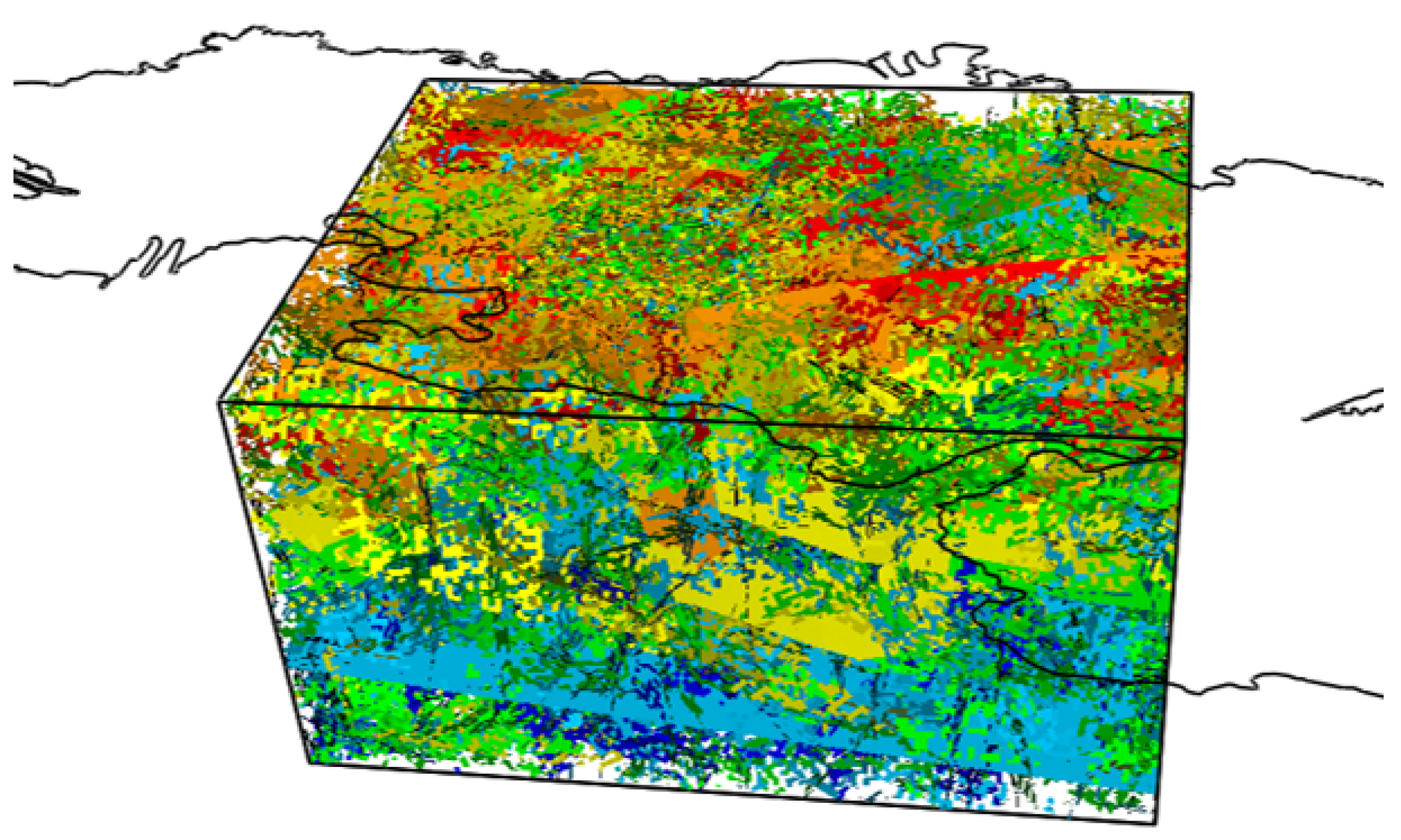
3.5. Meteoric Water Penetration at Olkiluoto Island

Olkiluoto Island is the location of the Finnish spent nuclear fuel repository, which is currently under construction. It has an area of about 12 km² and is bounded by brackish seawater. The island is largely flat with elevations mostly below 10 m. Precipitation infiltrates down to the crystalline bedrock, driven by the surface topology. These groundwater flows occur within a network of connected fractures. The fractures were generated by various regional tectonic events occurring during the Precambrian period. Drill-hole fracture data was analysed in [23] to determine an empirical relation between the intensity and transmissivity of bedrock fractures, and depth.

The salinities of the groundwaters at Olkiluoto have been shown to have a clear dependence on depth [24]. Fresh water of meteoric origin is prevalent at shallow depths; mixtures of glacial meltwater and Littorina Sea water are found at depths of −200 to −300 m; the groundwaters increase in salinity at even greater depths. Brines with salinities greater than 100 g/L are found below −900 m elevation, and their high density means they are mostly immobile. It is also noted in [24] that the distinct change in groundwater composition at −300 m elevation coincides with a notable decrease in the intensity and transmissivity of percolating fractures. Given these findings, it is likely that the composition of groundwater, at depth, has been stable for several glacial cycles of the Quaternary period.

Analytical calculations and ECPM transient multi-component solute transport calculations are used in [12] to predict how the groundwater salinity may evolve in the bedrock around the repository. Circulation of groundwater to depth was found to be limited by the decrease in fracture transmissivity at depth and also the large proportion of sub-horizontal fracturing.

The Olkiluoto repository is located at −410 m elevation. A site-scale model with dimensions 2.7 km by 2.1 km and 1.4 km depth has previously been developed in [22]. Around the repository, smaller fractures (greater than 20 m in length) are included in the model. Further from the repository, only (hydraulically active) deformation zones are included, together with fractures greater than 200 m in length (Figure 8). The fracture properties are as described in the Olkiluoto Case C DFN model from the 2011 site-descriptive modelling (SDM) [23] and the TURVA-2012 safety assessment [25]. The resulting model includes channelling and discontinuities within the fracture planes. There are approximately 30,000 fractures overall and when tessellated there are 460,000 sub-fractures. The fracture statistics are summarised in

Table 7. Fracture statistics for the Olkiluoto model.

Property	Value	Units
Number of fractures	29,012
Number of sub-fractures	461,687
Total fracture area per unit volume (P32)	2.02 × 10−2	m−1
P32 for Hydrozone (averaged over model)	2.56 × 10−3	m−1
Tessellation length	20	m

.

Simulations have been carried out using this model to represent the displacement of saline groundwater by meteoric water for a period of two thousand years of the current temperate period. The simulations include variable-density flow, dispersion, diffusion, and advection within the fracture network. Two reference waters are used in the model, whose properties are provided in

Table 8. Properties used in the Olkiluoto model for the two reference waters. Properties with an asterisk are specified at standard temperature and pressure. The density and viscosity are calculated from the salinity using an empirical expression from [16].

	Description	Saline Concentration (kg/m3) *	Density (kg/m3) *	Viscosity (Pa.s) *	Salinity (g/kg)
Ref. water A	Brine	77.50	1051.4	1.128 × 10−3	73.71
Ref. water B	Meteoric	2.42	999.9	1.005 × 10−3	2.420

. The calculations are post-closure and do not include pumping during the operation or construction of the repository.

A static temperature distribution is used, which increases linearly. At sea level, the temperature is 6 °C and at −1400 m elevation it is 25.7 °C. The longitudinal dispersion length is 20 m, and this is the same as the tessellation length used to subdivide the fractures. The transverse dispersion length is 5 m. RMD is included in the model, with parameters given in

Table 9. Rock matrix diffusion related parameters. The flow wetted surface is calculated during the upscaling process from the fracture area within each cell.

Property	Symbol	Value
Porosity of matrix	$\alpha$	0.005
Intrinsic diffusion coefficient	$D_i$	6 × 10−14 m2/s
Flow wetted surface (ECPM)	$\sigma$	3.238 m2/m3 (0 to −50 m depth) 0.692 m2/m3 (−50 m to −150 m) 0.698 m2/m3 (−150 m to −400 m) 0.372 m2/m3 (below −400 m)
Matrix diffusion length	$w_{max}$	$\raisebox{1ex}{$1$}\!\left/ \!\raisebox{-1ex}{$\sigma $}\right.$ (Random fractures)
Number of RMD finite volumes	$n_{fv}$	5
Finite volume lengths	$w_i$	$\raisebox{1ex}{$w_{max}$}\!\left/ \!\raisebox{-1ex}{$5$}\right.$

.

Table 10. Boundary conditions used in the Olkiluoto models. Note that the physical system would have flow through the sides of the model, but no-flow boundary conditions have been used as a simplification.

Surface	Concentration	Pressure
Top	Initial value	Initial value
Sides	Initial value	Zero flow
Bottom	Initial value	Zero flow

summarises the boundary conditions applied to the model. Initial value boundary conditions fix the pressures and concentrations on the boundary equal to the initial condition, throughout the calculation.

An ECPM regional-scale simulation of the Olkiluoto site is presented in [26] for the period 6000 BC to 2000 AD. That calculation was calibrated such that the end point reasonably matched current day observations of groundwater composition. Hence, the final timestep of that calculation is a convenient starting point for the simulations of the future evolution of the site presented here (interpolation is used to map from the ECPM to the DFN). The initial salt concentrations within the fractures and the rock matrix are identical.

The fracture network described above has also been upscaled to produce a site-scale ECPM model (distinct from the regional scale ECPM model developed in [26]). The flow-based upscaling was used to determine the permeability tensor, the kinematic porosity and fracture area per unit volume (for the RMD calculation). Prior to the upscaling, unconnected fractures were removed. The resulting ECPM mesh has around one million 20 m by 20 m by 20 m hexahedral cells. A minimum permeability of 10⁻¹⁸ m² and a minimum porosity of 10⁻⁴ is enforced in cells containing no fractures. The ECPM and DFN calculations have similar run-times for the resolutions used here.

Figure 9 presents results from both the DFN and ECPM models over a 2000-year period. This period is sufficient to show the composition changing at repository depth. Given the relatively small model domain, the simulation period cannot be extended while keeping the lateral boundary conditions fixed. Longer periods could be simulated if the boundary conditions were evolved or the model domain extended. The intrusion of meteoric water down towards the centre of the model is clear for both calculations. At repository depth saline water is displaced towards the lateral boundaries of the model. Comparing the DFN and ECPM models, the results are very similar. There are some differences which are thought to be due to the approximations made in the ECPM method. Upscaling may result in additional unphysical connectivity within a single ECPM cell [5]. This can lead to greater flow rates and/or a greater mixing of solutes between adjacent fractures. Conversely, upscaling sums the porosity of fractures within each cell, even parts of fractures that are not percolating; in some instances, this additional porosity can slow the rate of transport.

While these calculations suggest there is a degree of penetration of dilute water at the repository, the model is intended to be an illustrative demonstration of capability and includes simplifications with respect to the boundary conditions and the initial conditions. The initial matrix concentration is assumed to be equal to that in the fracture pore-water which will result in lower retardation of dilute water penetration to depth. The boundary conditions are all Dirichlet, which will become unphysical as the transient simulation progresses over time. Specifically, since the concentration boundary conditions cannot evolve in time, they will increasingly (and artificially) hinder the expected penetration of dilute water to repository depth.

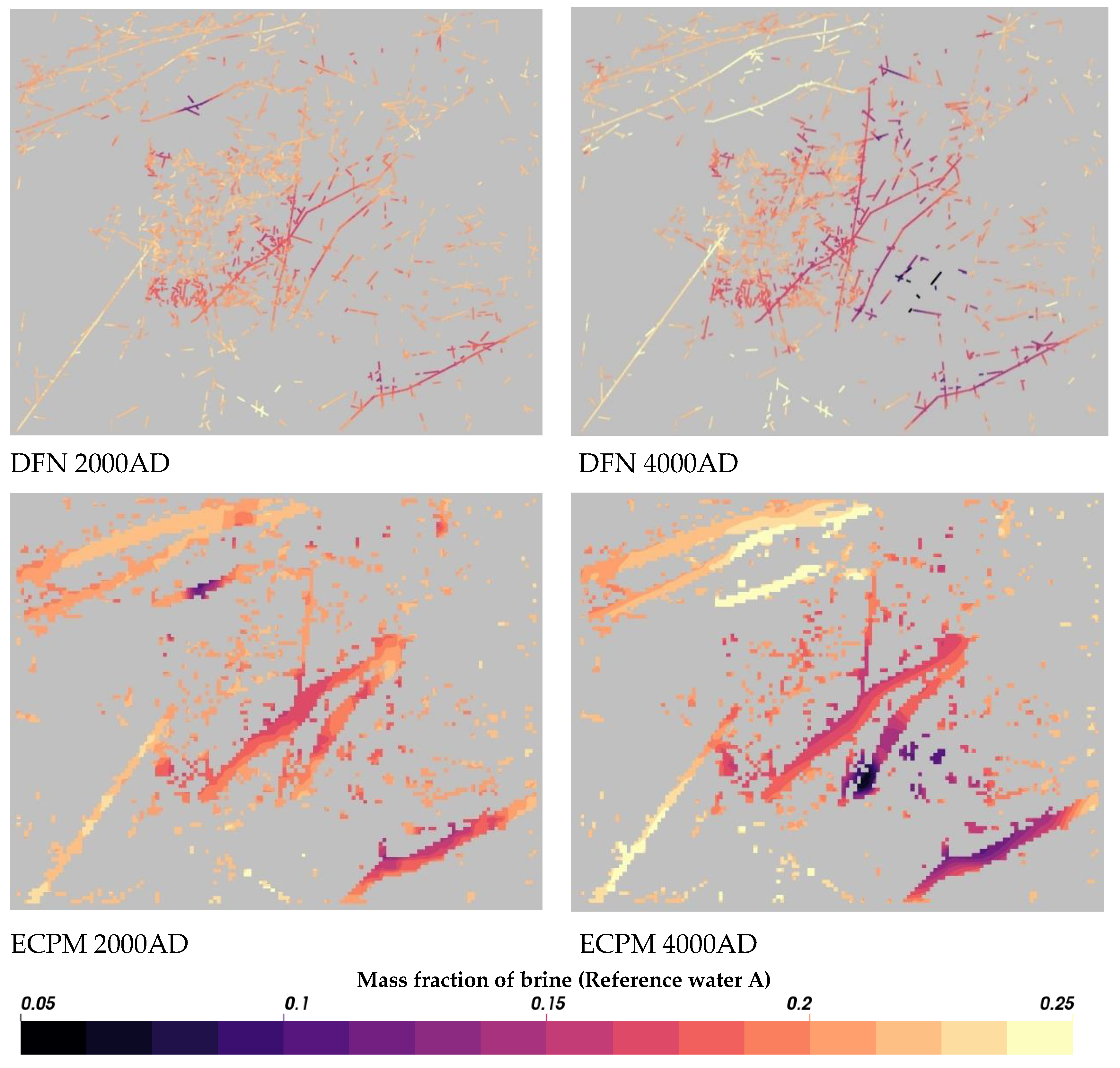
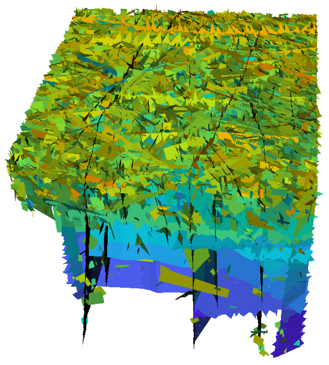
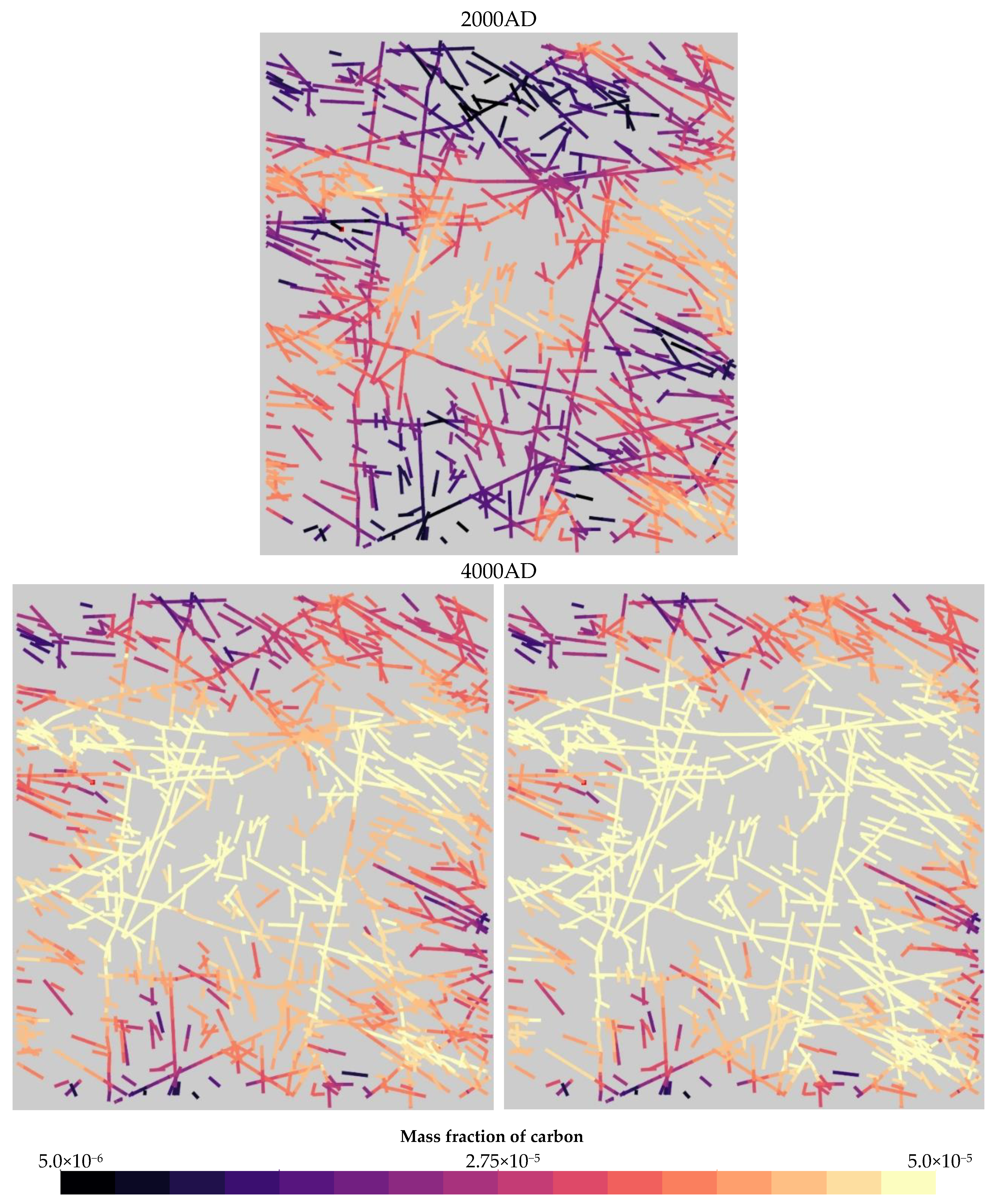
3.6. Laxemar Repository-Scale Model

Laxemar in Sweden was a candidate site for a spent nuclear fuel repository. At repository depth, groundwater flow occurs predominantly within a network of fractures in the crystalline bedrock.

An illustrative repository-scale model, based on the SR-Site Elaborated Laxemar Hydro-DFN [27,28], has been created. This model is 2.2 km by 2.2 km and extends 2.2 km below ground-surface. A discrete fracture network is used (see Figure 10) and includes deterministic fractures corresponding to brittle deformation zones and random fractures larger than 50 m. In total, there are about 14,000 fractures. All fractures are tessellated into smaller fractures with a tessellation length of 50 m. This results in 78,000 fracture tessellates.

The groundwater at repository depth is saline and calculations have been carried out to simulate the displacement and dilution of this water by meteoric water over the next two thousand years. The processes of advection, diffusion and dispersion within the fracture volume are included together with rock matrix diffusion. The transport and flow equations are coupled together via the density and viscosity. The equilibrium reaction for calcite has been included.

An ECPM regional-scale simulation of the Laxemar site, from 8000 BC to 2000 AD, is presented in [28]. The final time step from that model is used to define the current site-scale model’s initial conditions. The concentration in the rock matrix is initially identical to the concentration in the fractures. The boundary conditions for the site-scale model are the same as those specified for the Olkiluoto model in Table 10.

Figure 11 presents evolution for carbon concentration within the Laxemar model. Cross-sections through the model are shown at −490 m depth (the potential repository depth). Inorganic carbon concentrations (within the fracture) are significantly affected by these reactions. Over time the carbon concentration increases in the centre of the model due to the penetration of bicarbonate-rich meteoric water. The precipitation of calcite reduces the transport of inorganic carbon to depth for the case that includes chemical reactions. This behaviour is also seen in Figure 12, which shows average carbon mass fraction versus depth for calculations with and without calcite transport.

It is emphasised that this model is intended to be an illustrative demonstration of capability and includes simplifications with respect to the boundary conditions and the initial conditions.

4. Conclusions

This work has described an efficient new method for calculating hydrogeochemical evolution, within a fracture network, using an explicit DFN representation. This novel approach enables, possibly for the first time, site-scale simulations of multi-solute transport and reactive transport within DFNs. The implementation extends ConnectFlow’s discrete fracture network module to incorporate the following:

• Transporting multiple solute species, coupled with the flow equation via the density and viscosity.
• An algorithm for calculating solute diffusion into the rock matrix (RMD) around each fracture.
• An interface with the iPhreeqc library to model chemical reactions involving solutes, rock minerals, and minerals on fracture/pore surfaces.
• The performance of ConnectFlow’s DFN module has also been significantly improved via parallelisation.

These developments have been verified by comparing DFN calculations with ECPM calculations and analytical solutions. Two larger illustrative calculations have been presented:

• Site-scale simulations of dilute water penetration at Olkiluoto including rock matrix diffusion.
• Repository scale calculations of dilute water penetration at Laxemar including calcite reactions and RMD. Over the 2000-year period simulated, freshwater ingress and calcite precipitation are both observed.

To provide a good approximation, high resolutions have been used for the ECPM calculations. ECPM calculations used for previous safety cases tend to use lower resolutions for two reasons. Firstly, the ECPM approximation can lead to unphysical connectivity [5] which can exaggerate groundwater flow rates and underestimate travel times, which is a cautious approximation in the context of a safety assessment. This is likely to be more noticeable for an ECPM with lower resolution. Secondly, by using lower resolutions, the simulations are more tractable. DFN simulations have been shown to provide results that are qualitatively similar to results from ECPM calculations. However, because the ECPM is more of an approximation, some notable differences exist in the results from the two approaches.

This new capability within ConnectFlow allows the use of explicit discrete fracture network representations of hydrogeochemical processes within fractured rock. This will be crucial for ascertaining the potential long-term evolution of groundwater compositions for the current generation of geological disposal facilities that are located within fractured rock.

References

1. SKB. Long-Term Safety for the Final Repository for Spent Nuclear Fuel at Forsmark; SKB Report TR-11-01; SKB: Solna, Sweden, 2011. [Google Scholar]
2. Salas, J.; José Gimeno, M.; Auqué, L.; Molinero, J.; Gómez, J.; Juárez, I. SR-Site—Hydrogeochemical Evolution of the Forsmark Site; SKB Report TR-10-58; SKB: Solna, Sweden, 2010. [Google Scholar]
3. Trinchero, P.; Román-Ross, G.; Maia, F.; Molinero, J. Posiva Safety Case Hydrogeochemical Evolution of the Olkiluoto Site; Posiva Working Report 2014-09; Posiva Oy: Eurajoki, Finland, 2014. [Google Scholar]
4. Joyce, S.; Applegate, D.; Appleyard, P.; Gordon, A.; Heath, T.; Hunter, F.; Hoek, J.; Jackson, P.; Swan, D.; Woollard, H. Groundwater Flow and Reactive Transport Modelling in ConnectFlow; SKB Report R-14-19; SKB: Solna, Sweden, 2014. [Google Scholar]
5. Joyce, S.; Simpson, T.; Hartley, L.; Applegate, D.; Hoek, J.; Jackson, P.; Roberts, D.; Swan, D. Groundwater Flow Modelling of Periods with Temperate Climate Conditions—Laxemar; SKB Report R-09-24; SKB: Solna, Sweden, 2010. [Google Scholar]
6. Gylling, B.; Trinchero, P.; Molinero, J.; Deissmann, G.; Svensson, U.; Ebrahimi, H.; Hammond, G.E.; Bosbach, D.; Puigdomenech, I. A DFN-based High Performance Computing approach to the simulation of radionuclide transport in mineralogically heterogeneous fractured rocks. In Proceedings of the AGU Fall Meeting, San Francisco, CA, USA, 12–16 December 2016. [Google Scholar]
7. Pekala, M.; Wersin, P.; Pastina, B.; Lamminmäki, R.; Vuorio, M.; Jenni, A. Potential impact of cementitious leachates on the buffer porewater chemistry in the Finnish repository for spent nuclear fuel—A reactive transport modelling assessment. Appl. Geochem. 2021, 131, 105045. [Google Scholar] [CrossRef]
8. Repina, M.; Bouyer, F.; Lagneau, V. Reactive transport modeling of glass alteration in a fractured vitrified nuclear glass canister: From upscaling to experimental validation. J. Nucl. Mater. 2020, 528, 151869. [Google Scholar] [CrossRef]
9. Svensson, U.; Voutilainen, M.; Muuri, E.; Ferry, M.; Gylling, B. Modelling transport of reactive tracers in a heterogeneous crystalline rock matrix. J. Contam. Hydrol. 2019, 227, 103552. [Google Scholar] [CrossRef] [PubMed]
10. Khafagy, M.M.; Abd-Elmegeed, M.A.; Hassah, A.E. Simulation of reactive transport in fractured geologic media using ran-dom-walk particle tracking method. Arab. J. Geosci. 2020, 13, 34. [Google Scholar] [CrossRef]
11. Trinchero, P.; Puigdomenech, I.; Molinero, J.; Ebrahimi, H.; Gylling, B.; Svensson, U.; Bosbach, D.; Deissmann, G. Continu-um-based DFN-consistent simulations of oxygen ingress in fractured crystalline rocks. In Proceedings of the AGU Fall Meeting, San Francisco, CA, USA, 12–16 December 2016. Abstract #H13N-02. [Google Scholar]
12. Hoek, J.; Hartley, L.; Baxter, S. Hydrogeological Modelling for the Olkiluoto KBS 3H Safety Case; Posiva Working Report WR-2016-21; Posiva Oy: Eurajoki, Finland, 2016. [Google Scholar]
13. Sherman, T.; Sole-Mari, G.; Hyman, J.; Sweeney, M.R.; Vassallo, D.; Bolster, D. Characterizing Reactive Transport Behavior in a Three-Dimensional Discrete Fracture Network. Transp. Porous Media 2021. [Google Scholar] [CrossRef]
14. Vu, P.T.; Ni, C.-F.; Li, W.-C.; Lee, I.-H.; Lin, C.-P. Particle-Based Workflow for Modeling Uncertainty of Reactive Transport in 3D Discrete Fracture Networks. Water 2019, 11, 2502. [Google Scholar] [CrossRef]
15. Sudicky, E.A.; Frind, E.O. Contaminant Transport in Fractured Porous Media: Analytical Solutions for a System of Parallel Fractures. Water Resour. Res. 1982, 18, 1634–1642. [Google Scholar] [CrossRef]
16. Kestin, J.; Khalifa, E.; Correia, R. Tables of the dynamic and kinematic viscosity of aqueous NaCl solutions in the temperature range 20–150 °C and the pressure range 0.1–35 MPa. J. Phys. Chem. Ref. Data 1981, 10, 71. [Google Scholar] [CrossRef]
17. ConnectFlow Website. Available online: https://www.connectflow.com/resources/docs/conflow_technical.pdf (accessed on 28 February 2022).
18. Galerkin, B.G. Rods and Plates, Series Occurring in Various Questions Concerning the Elastic Equilibrium of Rods and Plates. Vestnik Inzhenerov i Tekhnikov 1915, 19, 897–908. English Translation: 63-18925, Clearinghouse Fed. Sci. Tech. Info.1963. (In Russian) [Google Scholar]
19. Cordes, C.; Kinzelbach, W. Continuous Groundwater Velocity Fields and Path Lines in Linear, Bilinear, and Trilinear Finite Elements. Water Resour. Res. 1992, 28, 2903–2911. [Google Scholar] [CrossRef]
20. Neretnieks, I. Diffusion in the rock matrix: An important factor in radionuclide retardation? J. Geophys. Res. 1980, 85, 4379–4397. [Google Scholar] [CrossRef] [Green Version]
21. Charlton, S.R.; Parkhurst, D.L. Modules Based on the Geochemical Model PHREEQC for Use in Scripting and Pro-gramming Languages. Comput. Geosci. 2011, 11, 1653–1663. [Google Scholar] [CrossRef]
22. Applegate, D.; Appleyard, P.; Joyce, S. Modelling Solute Transport and Water-Rock Interactions in Discrete Fracture Networks; Posiva Working Report WR-2020-01; Posiva Oy: Eurajoki, Finland, 2020. [Google Scholar]
23. Hartley, L.; Appleyard, P.; Baxter, S.; Hoek, J.; Roberts, D.; Swan, D. Development of a Hydrogeological Discrete Fracture Network Model of Olkiluoto; Site Descriptive Model 2011; Posiva Working Report WR-2012-32; Posiva Oy: Eurajoki, Finland, 2012. [Google Scholar]
24. Smellie, J.; Pitkänen, P.; Koskinen, L.; Aaltonen, I.; Eichinger, F.; Waber, F.; Sahlstedt, E.; Siitari-Kauppi, M.; Karhu, J.; Löfman, J.; et al. Evolution of the Olkiluoto Site: Palaeohydrogeochemical Considerations; Posiva Working Report WR-2014-27; Posiva Oy: Eurajoki, Finland, 2014. [Google Scholar]
25. Posiva. Nuclear Waste Management at Olkiluoto and Loviisa Power Plants: Review of Current Status and Future Plans for 2013–2015; Posiva Report YJH-2012; Posiva Oy: Eurajoki, Finland, 2012. [Google Scholar]
26. Posiva. Modelling Hydrogeochemical Evolution for the Olkiluoto KBS-3H Safety Case; Posiva Report 2016-11; Posiva Oy: Eurajoki, Finland, 2017. [Google Scholar]
27. SKB. Summary of Discrete Fracture Network Modelling as Applied to Hydrogeology of the Forsmark and Laxemar Sites; SKB Report SKB R-12-04; SKB: Solna, Sweden, 2013. [Google Scholar]
28. SKB. SFL—Groundwater Flow and Reactive Transport Modelling of Temperate Conditions; SKB Report SKB R-19-02; SKB: Solna, Sweden, 2019. [Google Scholar]
Figure 1. In ConnectFlow, DFN simulations are performed in two steps. Firstly, a series of calculations are done for each individual fracture (each calculation determines a global basis function). The global basis functions are then used to build the global equations which are then solved.
Energies 15 06199 g001
Figure 2. Example of ConnectFlow’s regular triangular finite element discretisation as used for fractures. Intersections are approximated using the lines formed by the boundaries of the triangular elements on the fracture. The regular finite element mesh can be solved very efficiently.
Energies 15 06199 g002
Figure 3. Schematic of transport within the fracture and the matrix. The blue arrows indicate advective-diffusive transport between sub-fractures; the black arrows indicate diffusive transport between the fracture and the matrix, and also within the matrix.
Energies 15 06199 g003
Figure 4. An idealised system of regularly spaced fractures embedded in a porous matrix (adapted from [15]).
Energies 15 06199 g004
Figure 5. (TOP) Stochastic fractures in a cuboid block, coloured by transmissivity. (BOTTOM) The equivalent CPM for the fractures, coloured by permeability. For clarity, cells whose permeability is less than 10−18 m2 have been removed. Reprinted with permission from [22], 2020, Posiva Oy.
Energies 15 06199 g005
Figure 6. Concentrations halfway along the block at x = 250 m. DFN and ECPM cases are both shown, both with and without RMD.
Energies 15 06199 g006
Figure 7. Comparison of carbon mass fraction for DFN and CPM cases (almost exact agreement) with and without chemical reactions. The mass fractions are measured halfway along the fracture. Reprinted with permission from [22], 2020, Posiva Oy.
Energies 15 06199 g007
Figure 8. The site-scale fracture network used for the DFN model for Olkiluoto. The outline of the island is included in black for context. Blues denote lower transmissivities and reds show higher transmissivities. Reprinted with permission from [22], 2020, Posiva Oy.
Energies 15 06199 g008
Figure 9. Horizontal slices of concentration at −410 m depth. These show the salinity evolution at the Olkiluoto site for a 2000-year period. Two models are shown, ECPM (bottom) and DFN (top). Both cases include rock matrix diffusion.
Energies 15 06199 g009
Figure 10. The fracture network used for the Laxemar calculations. Darker blues denote low transmissivites, and greens and yellows denote higher transmissivities.
Energies 15 06199 g010
Figure 11. Inorganic carbon mass fractions for a horizontal cross-section at −490 m elevation for the Laxemar model. The image on the left includes chemical reactions and the image on the right does not.
Energies 15 06199 g011
Figure 12. Average mass fraction of carbon (averaged over the central 1 km2 of the model) versus depth for calculations with and without chemical reactions involving calcite.
Energies 15 06199 g012