Adaptive PI and RBFNN PID Current Decoupling Controller for Permanent Magnet Synchronous Motor Drives: Hardware-Validated Results

Abstract

This study presents an adaptive proportional-integral (PI) and radial basis function neural network proportional-integral-derivative (PID) current control solution for permanent magnet synchronous motor (PMSM) drives. The proposed controller includes four controls: a decoupling term, a PI term, a supervision term, and a radial basis neural network-PID (RBFNN-PID) term. The first control term makes up the nonlinear factors, the second automatically adjusts the control gains, the third guarantees the system stability, and the fourth optimizes the PID parameters to achieve optimal system performance. Unlike off-line tuned PID controllers, the adaptive controller includes an adaptive tuning method for the on-line adjustment of control gain based on the gradient descent strategy. Therefore, it can be adjusted and handle the uncertainty of any system parameters. The program is not only simple and easy to be implemented but also ensures the accuracy and rapidity of the tracking speed. The control system has proven to be asymptotically stable. To verify the theory and application of the algorithm, a comparative experiment between the adaptive PI + RBFNN-PID controller and traditional PI + PID controller was conducted, demonstrating good robustness, which can effectively improve the PMSM. The results confirm that the proposed design achieves excellent control stability (i.e., quicker transient responding and smaller steady state error) in the presence of parametric uncertainty compared to conventional PID methods.

1. Introduction

Currently, AC motors are widely used in household appliances and industrial fields, with examples including power cars, wind power systems, industrial robotics, air conditioning (ac), and washing machines. There are two main types of AC motors: asynchronous motor (IM) and PMSM. About 70% of industrial motors are IM because of its simplicity, durability, and low production cost [1,2,3,4,5]. However, the permanent magnet synchronous motor (PMSM) is gradually replaced by people because of its high efficiency, low maintenance cost and high power density. However, the permanent magnet synchronous motor (PMSM) system is a nonlinear multivariable system whose performance is not easy to control due to changes in operating parameters [6,7,8,9]. Therefore, it is necessary to develop a high-performance controller with a simple algorithm, quick response time, extremely high precision and strong robustness. The motor parameters and load torque variations of a proportional-integral-differential (PID) controller are used to operate permanent magnet synchronous motor (PMSM) system in industry because of its simplicity, definitude of function and high efficiency [10]. However, one of the main problems with conventional PID controllers is sensitivity to the uncertainties of the system. Therefore, the control performance of traditional PID methods is severely degraded due to parameter changes. Some researchers surmount this shortcoming by designing mixed PID controllers or new adjusting rules [11,12,13]. As shown in [11], a mixed control system consisting of a transient fuzzy controller and a steady-state PI controller is proposed. Additionally [12] adjusted PI gain with fuzzy rules. However, these two methods both use off-line adjustment rules and lack adaptability to the uncertainty of time-varying systems in contrast to the adaptive PI controller with on-line regulation shown in [13]. Although the controller did not require any precise knowledge of motor parameters, there were no tested uncertain parameters. Recently, several researchers have proposed many advanced control strategies including fuzzy logic control (FLC) with nonlinear optimal control for the effective control of PMSM systems, nonlinear optimal control (NOC) with sliding mode control (SMC), neural network control, and adaptive control FLC [14]. Because of its fuzzy reasoning ability [15] has become a research hotspot. However, as the number of fuzzy rules adds, the control precision becomes greater, but the control algorithm becomes increasingly complex. NOC has been successfully introduced and applied to PMSM controllers [16,17]. Unfortunately, these controllers need sufficient knowledge and accuracy of motor parameters and has not yet been tested with drastic changes in mechanical parameters. Because of its robustness to external load disturbance and fast dynamic response, SMC is widely used in the speed control of permanent magnet synchronous motors [18,19,20,21]. Yet, the system dynamics are still susceptible to parameter changes and flutter problems. At the same time, another design method of speed control using NNC for permanent magnet synchronous motor system has been proposed [22,23,24]. One of the most important features of this technique is its advantage to approach linear or non-linear mappings by learning. Though its high complexity results in the control algorithm limits its implementation in practical applications. Adaptive control is another interesting approach because it can handle variable motor parameters and load torque for permanent magnet synchronous motor drives as shown in [25,26]. However, these two studies only considered changes in stator inductance and load torque. Other motor parameters present uncertainty such as stator resistance, moment of inertia, and viscous friction coefficient. In addition, convergence conditions for system dynamic errors are not guaranteed for the adaptive control algorithm [26].

This study combines the simple and effective traditional PI + PID controller with the self-tuning capabilities of adaptive control to designed a better adaptive PI + RBFNN-PID controller for permanent magnet synchronous motor drives. The controller contains an adaptive tuning law designed to tune the control gain on-line using the method of gradient descent. Thus, when the parameters are changed, the PI + PID-RBFNN gain will be auto-adjusted to the optimal value. Therefore, good dynamic response can be obtained even when the system parameters are uncertain. The Lyapunov stability theory describes the stability analysis of the proposed control strategy in detail. The experimental results for the current fluctuation and current response time show that the proposed adaptive PI + RBFNN-PID control scheme is effective and feasible when compared with the traditional PI + PID control scheme under the condition of uncertain parameters. In Section 2, the model is defined. In Section 3, the adaptive PI and PID controllers are defined, and the performance is analyzed. In Section 4, the RBFNN-PID controller is defined, and the performance and advantage of the NN compensator from RBFNN-PID is verified. In Section 5, a comparison between the conventional PI + PID method and the proposed adaptive PI +RBFNN-PID method for the current fluctuation and current response time is completed.

2. System Dynamic Error and Model Description

2.1. The Model Description from the System

The torque balance equation of a PMSM [27] is:

$${\tau }_{em}=J_{eq}d{\omega }_m/dt+B_a{\omega }_m+T_L,$$

(1)

where $J_{eq}$ is the inertia of the motor; ${\omega }_m$ is the motor rotational speed; $B_a$ is the friction coefficient; $T_L$ is the load torque; and ${\tau }_{em}$ is the electromagnetic drive torque, which depends on the type of PMSM. For a PM motor, ${\tau }_{em}$ can be expressed as follows:

$${\tau }_{em}=P({\psi }_f{i}_{sq})\mathrm{PM}\mathrm{motor}$$

(2)

where P represents the number of motor pole pairs. Finally, the relationship between ${\omega }_m$ and ${\omega }_e$ is given by:

$${\omega }_e={\omega }_m\cdot P.$$

(3)

A mathematical model of a SMT permanent rotating reference frame motor driver can be described by the following equations in the d, q rotating reference frame

$$\{\begin{array}{l}{\dot{i}}_d=-\frac{R_s}{L_d}{i}_d+\frac{1}{L_d}{V}_d+{\omega }_e{i}_q\\ {\dot{i}}_q=-\frac{R_s}{L_q}{i}_q-\frac{{\psi }_f}{L_q}{\omega }_e+\frac{1}{L_q}{V}_q-{\omega }_e{i}_d\end{array},$$

(4)

where ${\omega }_e$ is the rotor speed of PMSM; $i_d$ and $i_q$ are the d and q stator current, respectively; $V_q$ and $V_d$ are the d and q voltage input, respectively; $L_d$ and $L_{\mathrm{q}}$ is the d and q stator inductance, respectively; $R_s$ is the stator resistance; and ${\psi }_f$ is the flux linkage.

2.2. The Dynamic Error System

To improve the stability of a PMSM, the errors and integral of errors are joined. The dynamic errors between $i_d$ and its reference value, $i_d^{*}$, and between $i_q$ and its reference value, $i_q^{*}$, are defined as:

$$\{\begin{array}{l}{e}_d=i_d^{*}-i_d\\ e_q=i_q^{*}-i_q\end{array}.$$

(5)

The integrals of $e_q$ and $e_d$ are defined as:

$$\{\begin{array}{l}{\delta }_d={\displaystyle {\int }_0^t{e}_d}dt\\ {\delta }_q={\displaystyle {\int }_0^t{e}_q}dt\end{array}.$$

(6)

A positive definite Lyapunov function is constructed as:

$$V=\frac{1}{2}{e}_d^2+\frac{1}{2}{e}_q^2+\frac{1}{2}{k}_{id}{\delta }_d^2+\frac{1}{2}{k}_{iq}{\delta }_q^2.$$

(7)

The derivative of $V$ to $t$ gives the following result:

$$\begin{array}{l}\dot{V}=e_d[{\dot{i}}_d^{*}-\frac{1}{L_d}(u_d-R_s{i}_d+{\omega }_e{L}_q{i}_q)+k_{id}{\delta }_d]\\ +e_q[{\dot{i}}_q^{*}-\frac{1}{L_q}(u_q-R_s{i}_q-{\omega }_e{L}_d{i}_d-{\omega }_e{\psi }_f)+k_{iq}{\delta }_q],\end{array}$$

(8)

$$\{\begin{array}{l}{V}_d=L_d{\dot{i}}_d^{*}+R_s{i}_d+k_1{L}_d{e}_d+k_{id}{L}_d{\delta }_d\\ -{\omega }_e{L}_q{i}_q\\ V_q=L_q{\dot{i}}_q^{*}+R_s{i}_q+k_2{L}_q{e}_q+k_{iq}{L}_q{\delta }_q\\ +{\omega }_e{L}_d{i}_d+{\omega }_e{\psi }_f\end{array},$$

(9)

$$\{\begin{array}{l}{V}_d=L_d{\dot{i}}_d+R_s{i}_d+L_d{\dot{e}}_d+k_1{L}_d{e}_d+k_{id}{L}_d{\delta }_d-{\omega }_e{L}_q{i}_q\\ V_q=L_q{\dot{i}}_q+R_s{i}_q+L_q{\dot{e}}_q+k_2{L}_q{e}_q+k_{iq}{L}_q{\delta }_q\\ +{\omega }_e{L}_d{i}_d+{\omega }_e{\psi }_f\end{array}.$$

(10)

3. Design of the Adaptive PI and PID Controller

3.1. Traditional PI and PID Compound Control with Decoupling Technology

The equation for $V_{dq}$ and the conventional adaptive PI design are as follows:

$$V_{dq}=u_1+u_2+u_{nn},$$

(11)

The voltage equation of the mathematical model of SPMSM is as follows:

$$\{\begin{array}{l}{u}_{1d}=L_d{\dot{i}}_d+R_s{i}_d-{\omega }_e{L}_q{i}_q\\ u_{1q}=L_q{\dot{i}}_q+R_s{i}_q+{\omega }_e{L}_d{i}_d+{\omega }_e{\psi }_f\end{array},$$

(12)

Depending on $R_s$, $L_d$, $L_q$, and ${\psi }_f$, the system parameters ${\beta }_1-{\beta }_5$ can be expressed as:

$${\beta }_1=\frac{R_s}{L_d},{\beta }_2=\frac{1}{L_d},{\beta }_3=\frac{R_s}{L_q},{\beta }_4=\frac{1}{L_q},{\beta }_5=\frac{{\psi }_f}{L_q}$$

(13)

The mathematical model of the current equation obtained by combining Equations (12) and (13) is:

$$\{\begin{array}{l}{\dot{i}}_d=-{\beta }_1{i}_d+{\beta }_2{u}_{1d}+{\omega }_e{i}_q\\ i_q=-{\beta }_3{i}_q+{\beta }_4{u}_{1q}-{\beta }_5{\omega }_e-{\omega }_e{i}_d\end{array},$$

(14)

where $u_1$, as shown in Equation (11), is as follows:

$$u_1=u_0+u_{PI}+u_s$$

(15)

From Equations (12) and (13), the models of the error system are as follows:

$$\{\begin{array}{l}{u}_{1d}=({\beta }_1{i}_d-{\omega }_e{i}_q)/{\beta }_2\\ u_{1q}=({\beta }_3{i}_q+{\beta }_5{\omega }_e+{\omega }_e{i}_d)/{\beta }_4\end{array},$$

(16)

From Equations (12), (14), and (16), Equation (14) is expressed as:

$$\{\begin{array}{l}{\dot{i}}_d={\beta }_2(u_{1d}-u_{0d})\\ i_q={\beta }_4(u_{1q}-u_{0q})\end{array},$$

(17)

$u_{1dq}$ can be rewritten in vector form as:

$$u_{1dq}=\left[\begin{array}{l}{\beta }_2{u}_{1d}\\ {\beta }_4{u}_{1q}\end{array}\right]=A\left[\begin{array}{l}{u}_{1d}\\ u_{1q}\end{array}\right]=u_0+u_{PI},$$

(18)

The value of the coefficient A is as follows:

$$A=\left[\begin{array}{cc}{\beta }_2& 0\\ 0& {\beta }_4\end{array}\right],$$

(19)

The value of the coefficient $u_{PI}$ is as follows:

$$\begin{array}{l}{u}_{PI}=\left[\begin{array}{l}{u}_{1PI}\\ u_{2PI}\end{array}\right]=\left[\begin{array}{l}-K_{1P}{i}_d-K_{1I}{\displaystyle {\int }_0^t{i}_{d}dt}\\ -K_{2P}{i}_q-K_{2I}{\displaystyle {\int }_0^t{i}_{q}dt}\end{array}\right],\\ =EK\end{array}$$

(20)

where $K_{1P},K_{1I},K_{2P},K_{2I}$ are the proportional gain, integral gain and differential gain of the PI controller, respectively. The equation of state and gain matrices are expressed as:

$$E=\left[\begin{array}{c}\begin{array}{cc}\begin{array}{cc}\begin{array}{cc}{\displaystyle {\int }_0^t{i}_{d}dt}& i_d\end{array}& 0\end{array}& 0\end{array}\\ \begin{array}{cc}\begin{array}{cc}\begin{array}{cc}0& 0\end{array}& {\displaystyle {\int }_0^t{i}_{q}dt}\end{array}& i_q\end{array}\end{array}\right],$$

(21)

$$K={\left[\begin{array}{cccc}-K_{1I}& -K_{1P}& -K_{2I}& -K_{2P}\end{array}\right]}^{{\rm T}},$$

(22)

It is important to note that the derivative of the current model is usually convoluted and, therefore, was excluded in Equation (22).

Adaptive PI relies on on-line parameter tuning, which solves the problem of matching the motor’s internal parameters and enables a rapid response system. The proposed adaptive PI controller can be expressed as:

$$u_{1dq}=u_0+u_{PI}-u_{PI0}+u_s.$$

(23)

3.2. The Proposed Adaptive PI Controller

The latest trajectory error vectors under the reduced-order dynamics of SMC are used to obtain an adaptive tracking error rule.

$$s(t)=\left[\begin{array}{c}{s}_1(t)\\ s_2(t)\end{array}\right]=\left[\begin{array}{c}{i}_d\\ i_q\end{array}\right].$$

(24)

From the viewpoint of sliding mode control, the conditions for the existence of sliding mode and collision mode are derived according to Lyapunov. In general, the Lyapunov candidate function for the SMC is expressed by $V_1=1/2s^{{\rm T}}s$. Then, the slip can be derived from the Lyapunov theory that can verify the slip of the system, which is given by:

$${\dot{V}}_1(t)=s^{{\rm T}}\dot{s}<0.$$

(25)

The SMC condition requires that $s\to 0$ as $t\to \infty$. To obtain the adaptive regulation of the PI gain, the supervised gradient method is used to decrease the SMC condition. The method of the gradient descent algorithm is computed in the opposite direction of the power flows and yields the stable characteristics of the PID gains. Therefore, the four adaptive laws governing the gain, $K_{1P}$, $K_{1I}$, $K_{2P}$, and $K_{2I}$, are easily obtained under the supervisory gradient method, that is as follows:

$$\begin{gathered} {\dot{K}}_{1P}=-{\gamma }_{1P}\frac{\partial V_1}{\partial K_{1P}}=-{\gamma }_{1P}\frac{\partial V_1}{\partial u_{1PI}}\frac{\partial u_{1PI}}{\partial K_{1P}}=-{\gamma }_{1P}{s}_1{i}_d, \\ {\dot{K}}_{1I}=-{\gamma }_{1I}\frac{\partial V_1}{\partial K_{1I}}=-{\gamma }_{1I}\frac{\partial V_1}{\partial u_{1PI}}\frac{\partial u_{1PI}}{\partial K_{1I}}=-{\gamma }_{1I}{s}_1{\displaystyle {\int }_0^t{i}_{d}dt}, \\ {\dot{K}}_{2P}=-{\gamma }_{2P}\frac{\partial V_1}{\partial K_{2P}}=-{\gamma }_{2P}\frac{\partial V_1}{\partial u_{2PI}}\frac{\partial u_{2PI}}{\partial K_{2P}}=-{\gamma }_{2P}{s}_2{i}_q, \\ {\dot{K}}_{2I}=-{\gamma }_{2I}\frac{\partial V_1}{\partial K_{2I}}=-{\gamma }_{2I}\frac{\partial V_1}{\partial u_{2PI}}\frac{\partial u_{2PI}}{\partial K_{2I}}=-{\gamma }_{2I}{s}_2{\displaystyle {\int }_0^t{i}_{q}dt}, \end{gathered}$$

(26)

where ${\gamma }_{1P},{\gamma }_{1I},{\gamma }_{2P},{\gamma }_{2I}$ are the learning rates that are positive.

The adaptive adjusting method can be expressed in the following vector form:

$$\dot{K}=\varphi E^{{\rm T}}s,$$

(27)

where $\varphi =diag({\gamma }_{1I},{\gamma }_{1P},{\gamma }_{2I},{\gamma }_{2P}).$

Remark 1.

Using on-line adjustment, the control gain can be adjusted automatically with the change of system parameters. Thus, the designed adaptive PID controller can overcome the drawbacks of all off-line adjustment methods and provide good performance without being affected by the uncertainty of the system parameters.

Next, a monitor is required to pull the dynamic error back to a predetermined bounded area and guarantee the stability of the system. Suppose there is an optimized PI control ($u_{PI}^{*}$) such that:

$$u_{PI}^{*}=u_{PI0}+\epsilon ,$$

(28)

where $K^{*}={\left[\begin{array}{cccc}-K_{1I}^{*}& -K_{1p}^{*}& -K_{2I}^{*}& -K_{2P}^{*}\end{array}\right]}^{{\rm T}}$ is the optimal gain matrix and $\epsilon ={\left[\begin{array}{cc}{\epsilon }_1& {\epsilon }_2\end{array}\right]}^{{\rm T}}$, where ${\epsilon }_1$ and ${\epsilon }_2$ are the approximation inaccuracies, and they are assumed to be bounded by $0\le \left|{\epsilon }_1\right|\le {\alpha }_1$ and $0\le \left|{\epsilon }_2\right|\le {\alpha }_2$, in which ${\alpha }_1,{\alpha }_2$ are the positive constants. Then, the projection for the regulatory controls is as follows:

$$u_s=\left[\begin{array}{c}-{\alpha }_1\ast \mathrm{sgn}(s_1)\\ -{\alpha }_2\ast \mathrm{sgn}(s_2)\end{array}\right].$$

(29)

Through integrating the decoupling control terms, the PID control terms with adaptive laws, and the supervisory control terms, the desired controller is obtained as $u_{1dq}=u_{0dq}+u_{PI}+u_s.$

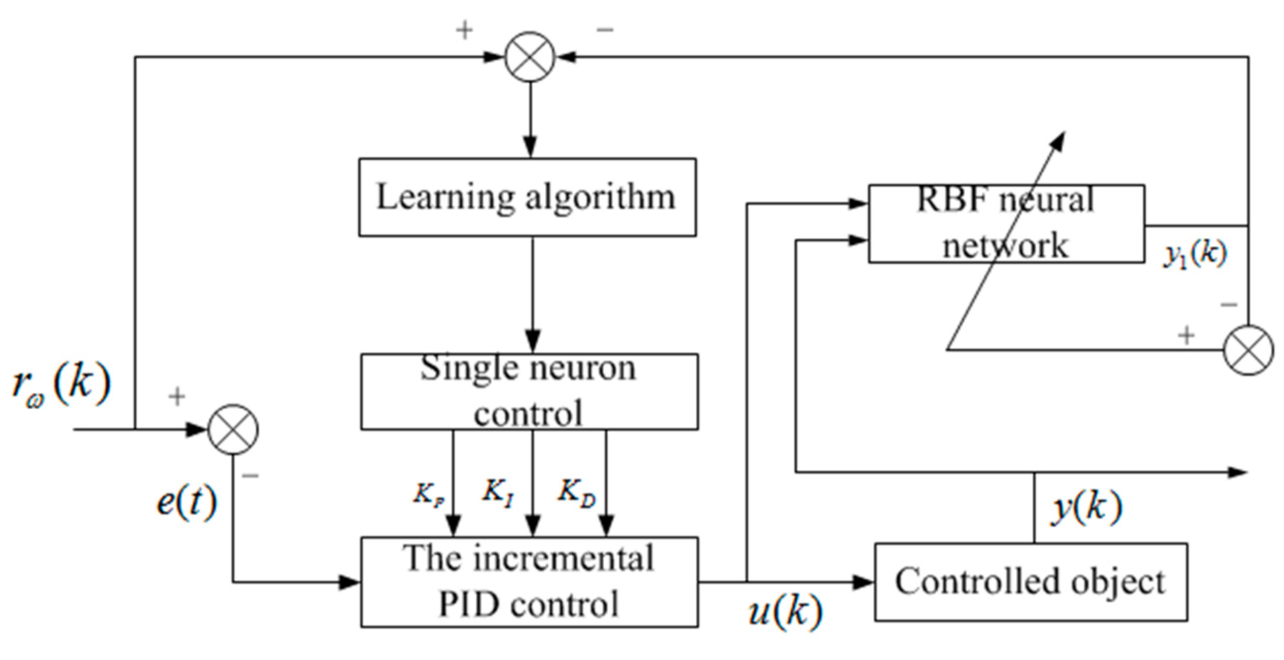
4. RBFNN-PID Controller Design

4.1. The Proposed Adaptive RBFNN-PID Controller

RBFNN incremental PID trajectory tracking is superior to traditional PID control in terms of adaptability, robustness and real-time performance. Unlike the conventional PID controller, it has a highly adaptive learning ability and meets the requirements for a nonlinear controller.

The expression of $u_2$ is:

$$u_2=u_{PID}+u_{2s},$$

(30)

$$\dot{e}=\sigma ,$$

(31)

$$\{\begin{array}{l}{u}_{2d}=L_d{\sigma }_d+k_1{L}_d{e}_d+k_{id}{L}_d{\delta }_d\\ u_{2q}=L_q{\sigma }_q+k_2{L}_q{e}_q+k_{iq}{L}_q{\delta }_q\end{array}.$$

(32)

$${\rm M}=\left[\begin{array}{c}\begin{array}{cc}\begin{array}{cc}\begin{array}{cc}\begin{array}{cc}\begin{array}{cc}{\delta }_d& e_d\end{array}& {\sigma }_d\end{array}& 0\end{array}& 0\end{array}& 0\end{array}\\ \begin{array}{cc}\begin{array}{cc}\begin{array}{ccc}\begin{array}{cc}0& 0\end{array}& 0& {\delta }_q\end{array}& e_q\end{array}& {\sigma }_q\end{array}\end{array}\right].$$

(33)

$${\rm Z}={\left[\begin{array}{cc}\begin{array}{cc}\begin{array}{cc}\begin{array}{cc}\begin{array}{cc}{Z}_{3I}& Z_{3P}\end{array}& Z_{3D}\end{array}& Z_{4I}\end{array}& Z_{4P}\end{array}& Z_{4D}\end{array}\right]}^{{\rm T}}.$$

(34)

The latest error tracking vector based on PID with the dynamics of SMC is given as:

$$\mathsf{\Omega }(t)=\left[\begin{array}{c}{\mathsf{\Omega }}_1(t)\\ {\mathsf{\Omega }}_2(t)\end{array}\right]=\left[\begin{array}{c}\frac{1}{s}{e}_d+e_d+s{e}_d\\ \frac{1}{s}{e}_q+e_q+s{e}_q\end{array}\right].$$

(35)

Then, the transfer function from $s_3$ is obtained by strictly positive real functions:

$$G(p)=\frac{e_d}{s_3}=\frac{1}{\frac{1}{s}+s+1},$$

(36)

where s is regarded as the Laplace variable. Therefore, it is to be stated that $e_d$ be astringent to zero when the condition of $s\to 0$ is satisfied.

$$\begin{gathered} {\dot{Z}}_{1P}=-{\eta }_{1P}\frac{\partial V_2}{\partial K_{3P}}=-{\eta }_{1P}{\mathsf{\Omega }}_1{e}_d, \\ {\dot{Z}}_{1I}=-{\eta }_{1I}\frac{\partial V_2}{\partial K_{3I}}=-{\eta }_{1I}{\mathsf{\Omega }}_1{\delta }_d, \\ {\dot{Z}}_{1D}=-{\eta }_{1D}\frac{\partial V_2}{\partial K_{3D}}=-{\eta }_{1D}{\mathsf{\Omega }}_1{\sigma }_d, \\ {\dot{Z}}_{2P}=-{\eta }_{2P}\frac{\partial V_2}{\partial K_{4P}}=-{\eta }_{2P}{\mathsf{\Omega }}_2{e}_q, \\ {\dot{Z}}_{2I}=-{\eta }_{2I}\frac{\partial V_2}{\partial K_{4I}}=-{\eta }_{2I}{\mathsf{\Omega }}_2{\delta }_q, \\ {\dot{Z}}_{2D}=-{\eta }_{2D}\frac{\partial V_2}{\partial K_{4D}}=-{\eta }_{2D}{\mathsf{\Omega }}_2{\sigma }_q, \end{gathered}$$

(37)

where ${\eta }_{1p},{\eta }_{1I},{\eta }_{1D},{\eta }_{2p},{\eta }_{2I},{\eta }_{2D}$ are the positive learning rates.

$$\dot{Z}=\xi {{\rm M}}^{{\rm T}}\mathsf{\Omega },$$

(38)

where $\xi =diag({\eta }_{3I},{\eta }_{3P},{\eta }_{3D},{\eta }_{4I},{\eta }_{4P},{\eta }_{4D}).$

Remark 2.

With on-line regulation, the control gain can be auto-adjustment as the system parameters change. Hence, the proposed RBFNN-PID controller can overcome the drawbacks of all off-line regulation methods and show good performance while ignoring the uncertainty of the system parameters.

$$u_{2s}=\left[\begin{array}{c}-{\alpha }_3\times \mathrm{sgn}(s_3)\\ -{\alpha }_4\times \mathrm{sgn}(s_4)\end{array}\right]$$

(39)

4.2. NN Compensator in RBFNN-PID

RBFNN is an efficient feedforward neural network, which has the characteristics of good approximation and generalization performance, a simple structure and fast learning speeds [28,29]. RBF neural network is used in the compensator, but it is not suitable for the multilayer neural network proposed in references [30,31,32]. The main structure of the RBFNN shown in the orange frames of Figure 1 consists of three layers [33]: an input layer with five variables, an output layer, $u^{*}$, and a hidden layer governed by a Gaussian function.

$$V^{*}=V_{qds}+u^{*}.$$

(40)

Layer one is the input layer. In this layer, inputs $x$ are to be used in the next layer.

$$\begin{gathered} x=\left[\begin{array}{cc}\begin{array}{cc}\begin{array}{cc}\begin{array}{cc}{\displaystyle {\int }_0^t{i}_d}& i_d\end{array}& {\delta }_d\end{array}& e_d\end{array}& {\dot{e}}_d\end{array}\begin{array}{cc}\begin{array}{cc}\begin{array}{cc}\begin{array}{cc}{\displaystyle {\int }_0^t{i}_q}& i_q\end{array}& {\delta }_q\end{array}& e_q\end{array}& {\dot{e}}_q\end{array}\right], \\ x=\left[\begin{array}{cc}\begin{array}{cc}\begin{array}{cc}\begin{array}{cc}{\displaystyle {\int }_0^t{i}_d}& i_d\end{array}& {\delta }_d\end{array}& e_d\end{array}& {\dot{e}}_d\end{array}\begin{array}{cc}\begin{array}{cc}\begin{array}{cc}\begin{array}{cc}{\displaystyle {\int }_0^t{i}_q}& i_q\end{array}& {\delta }_q\end{array}& e_q\end{array}& {\dot{e}}_q\end{array}\right], \end{gathered}$$

(41)

Layer two is the hidden layer—this layer consists of a series of computational cells of hidden neurons. Each neuron is activated by an RBF. The output of the hidden layer is computed by:

$$h_j(x,c,d)=\exp (-\frac{{\Vert x-c_j\Vert }^2}{2d_j^2}),j=1\dots m,$$

(42)

where m is the number of neurons; $c_j=\left[\begin{array}{cc}{c}_{j1}& c_{jn}\end{array}\right]$ is the center vector of neuron j; $d_j$ is the standard deviation of the $jth$ RBF, $d={\left[\begin{array}{cc}{d}_1& d_m\end{array}\right]}^{{\rm T}}$; and $h_j$ is the Gaussian function for neuron j.

Layer three is the export layer. The output indicator at this level is a linear weighted portfolio:

$$f(x)={\displaystyle \sum _{j=1}^m{W}_{ji}{h}_j(x,c,d),i=1\dots n},$$

(43)

where $W_{ji}$ refers to the weight, which connects the $jth$ hidden node to the $ith$ output, and n is the number of inputs.

In the designed neural network compensator, the input signal from layer one is the referred track vector, and the output from layer three is used for modeling difference, external disturbance and no modeling part. The NN compensator is used to create the non-linear projections between the referred track and the non-modeled dynamics, but it cannot achieve the whole optimal approximation. The center vector c and the standard deviation d are unchanged within the reference trajectory and the number of neurons. Because the radial basis function has the ability of nonlinear approximation, the best approximation $u^{*}$ can be described by:

$$u^{*}=f^{*}(x)-{\epsilon }_2=W^{*}h(x)-{\epsilon }_2,$$

(44)

where $f^{*}(x)$ is the output vector from the hidden layer; $W^{*}$ is the optimal weight value vector; and ${\epsilon }_2$ is a minimum approximating error. Due to the characteristics of the RBFNN, the following practical assumptions hold.

Assumption 1.

The approximation error${\epsilon }_2$is a small real constant. If the hidden layer has enough neurons, that is, the absolute value of${\epsilon }_2$can be any small number, i.e.,

$$\widehat{f}(x)=\widehat{W}h(x),$$

(45)

$$u^{*}=\widehat{f}(x)+\tilde{W}h(x)-{\epsilon }_2.$$

(46)

There is an optimal value$u_{nn}$that satisfies the following conditions$u^{*}$:

$$\{\begin{array}{l}{u}^{*}+f_d\le {\epsilon }_1\\ u^{*}(e+\delta +\sigma )\le 0\\ (e+\delta +\sigma )(u^{*}+f_d)\le \epsilon \end{array},$$

(47)

$$\widehat{f}(x)+\tilde{W}h(x)+f\le {\epsilon }_1+{\epsilon }_2=\epsilon ,$$

(48)

where$\tilde{W}=W^{*}-\widehat{W}$refers to the estimation error of the weight vector.

$u_{nn}$from Equation (11) satisfies the condition as:

$$\begin{gathered} u_{nn}=\widehat{f}(x)-v\tanh \left[\frac{v}{\sigma +e+\delta }\right]v>0, \\ {\dot{\widehat{W}}}_i=-{\mathsf{\Theta }}_i{h}_{i}p,i-1,2,\dots m, \\ p=\delta +e+\sigma , \end{gathered}$$

(49)

where${\mathsf{\Theta }}_i=diag\left[{\mathsf{\Theta }}_1,{\mathsf{\Theta }}_2\dots {\mathsf{\Theta }}_m\right]$is a positive symmetry theorem.

4.3. Stability and Analysis

To analyze system stability, the tracking theorem is as follows:

Theorem 1.

Regarding the dynamic error system represented by Equation (16). On the condition of applying with an adaptive PI + RBFNN-PID current controller, Equation (23), which having adaptive tuning method, Equation (26), the dynamic error system expresses asymptotically being stability.

Proof. 

The next equation can be deduced from Equations (16), (23), and (28):

$$\begin{array}{l}\dot{s}=B(u_{PI}+u_s-u_{{}_{PI}}^{*}+u_{{}_{PI}}^{*}-u_{PI0})\\ =B(E\tilde{K}+us-\epsilon ),\end{array}$$

(50)

where $\tilde{K}=K-K^{*}.$□

The control gain error is defined as follows:

$$\begin{gathered} {\tilde{K}}_{1P}=K_{1P}-K^{*}{}_{1P},{\tilde{K}}_{1I}=K_{1I}-K^{*}{}_{1I} \\ {\tilde{K}}_{2P}=K_{2P}-K^{*}{}_{2P},{\tilde{K}}_{2I}=K_{2I}-K^{*}{}_{2I}. \end{gathered}$$

(51)

On the basis of Equations (50) and (51), the following Lyapunov candidate functions were selected:

$$\begin{array}{l}{V}_2(t)=\frac{1}{2}{s}^T{B}^{-1}s+\frac{1}{{\gamma }_{1P}}{\tilde{K}}_{1P}^2+\frac{1}{{\gamma }_{1I}}{\tilde{K}}_{1I}^2\\ +\frac{1}{{\gamma }_{2P}}{\tilde{K}}_{2P}^2+\frac{1}{{\gamma }_{2I}}{\tilde{K}}_{2I}^2\end{array}$$

(52)

The Lyapunov function, $V_2(t)$, derivative of time is given by:

$$\begin{array}{l}{\dot{V}}_2(t)=\frac{1}{2}{s}^T{B}^{-1}\dot{s}+\frac{1}{{\gamma }_{1P}}{\tilde{K}}_{1P}{\dot{K}}_{1P}+\frac{1}{{\gamma }_{1I}}{\tilde{K}}_{1I}{\dot{K}}_{1I}\\ +\frac{1}{{\gamma }_{2P}}{\tilde{K}}_{2P}{\dot{K}}_{2P}+\frac{1}{{\gamma }_{2I}}{\tilde{K}}_{2I}{\dot{K}}_{2I}\\ =s^T{B}^{-1}B(E\tilde{K}+u_s-k)+{\tilde{K}}^T{\varphi }^{-1}\dot{\tilde{K}}\\ =s^T(E\tilde{K}-\left[\begin{array}{l}{\alpha }_1\mathrm{sgn}(s_1)\\ {\alpha }_2\mathrm{sgn}(s_2)\end{array}\right]-\epsilon )-{\tilde{K}}^T{\varphi }^{-1}\varphi E^{T}s\\ =-{\alpha }_1\left|s_1\right|-{\alpha }_2\left|s_2\right|-{\epsilon }_1{s}_1-{\epsilon }_2{s}_2\\ \le -({\alpha }_1-\left|{\epsilon }_1\right|)\left|s_1\right|-({\alpha }_2-\left|{\epsilon }_2\right|)\left|s_2\right|\\ \le 0.\end{array}$$

(53)

Using the adaptive PI controller, Equation (23), with adaptive tuning laws, Equation (26), for non-zero values, the relevant inequalities can be obtained for the tracking error vector $\dot{s}$, satisfied that ${\dot{V}}_2(t)$ is a negative semi-infinite function $\left[\mathrm{i}.\mathrm{e}.,V_2(t)\le V_2(0)\right]$, and s and $\tilde{K}$ must be bounded. The $\mathsf{\Omega }(t)$ can be expressed as $\mathsf{\Omega }(t)\equiv ({\alpha }_1-\left|{\gamma }_1\right|)\left|s_1\right|+({\alpha }_1-\left|{\gamma }_1\right|)\left|s_2\right|$, and the following inequality can be obtained from Equation (23):

$${\displaystyle {\int }_0^t\mathsf{\Omega }(\tau )}d\tau \le V_2(0)-V_2(t),$$

(54)

Since $V_2(0)$ and $V_2(t)$ are bounded and non-increasing, the following inequalities are deduced to be:

$$\underset{t\to \infty }{\lim }{\displaystyle {\int }_0^t\mathsf{\Omega }(\tau )}d\tau \le \infty .$$

(55)

Meanwhile, as long as s is bounded, Equation (25) indicates that V is also bounded. Then, $\mathsf{\Omega }(\tau )$ is uniform and continuous. By applying Barbalat’s lemma [34], it can be found that $\underset{t\to \infty }{\lim }\mathsf{\Omega }(\tau )=0$. Therefore, $s\to 0$ as $t\to \infty$ and the adaptive PI + RBFNN-PID controller will keep asymptotic stability even if the parameters of the motor change and external load disturbance occurs.

Remark 3.

It should be noted that the adaptive PI control strategy proposed in this paper is suitable for various electrical systems, and its mathematical form is shown in Equation (16). The general design process of the designed control strategy can be overviewed as follows.

Step one: Use the pole placement method [35,36] to select the initial value of the PI gain.

Step two: Structure the decoupling control term $u_{0d},$ and term $u_{0q}$ as Equation (14) and the supervision and control term $u_s$ as Equation (29).

Step three: Organize the PI control term $u_{PI}$ as Equation (20) with the self-adaptive control as Equation (26).

Step four: The desired laws from Equation (23) are obtained by combining the three controls in Equations (14), (20) and (29).

The stability analysis of RBFNN-PID is the same as the adaptive PI.

5. Experimental Validation

5.1. Drive System Settings

An experimental platform was set up with the core controller (TMS320F28335) from the TI company. The decoupling control of the PMSM was verified based on the current deviation control effect of the sliding mode control strategy. The program of the designed adaptive PI + RBFNN-PID control algorithm was followed as shown in Figure 2. The general design process of the control scheme was followed as shown in Figure 3, as proposed by F28335DSP, and the hardware was set up following the structure diagram of the all-digital control system based on the DSP as shown in Figure 4. The PMSM was a 400 W stepper motor drag model (YH57BYGH56). The PWM switching frequency of the DSP processor was set to 10 kHz, and the DC bus voltage provided by the output DC regulated power supply was set to 30V. The EPWM and RC filter circuit equivalent for the analog-to-digital conversion chip (ADC) and current analog signal output to the oscilloscope. The given parameters from the SPMSM controller are shown in

Table 1. Nominal SPMSM Parameters.

Parameter	Symbol	Value
Rated power	Pe	400 W
Rated phase-to-phase voltage	Vr	220 V
Rated phase current	Ir	2.8 A
Rated torque	Tr	2.7 N.M
Number of poles	P	8
Stator resistance	Rs	2.875 Ω
Stator inductance	Ld, Lq	0.22 mH, 0.61 mH
Magnet flux	ψf	0.085 V·s/rad
Equivalent inertia	J	0.0018 kg·m2
Viscous friction coefficient	B	0.0002 N·m·s/rad

.

5.2. Research Program

To evaluate the characteristics of the theory and application of the proposed control strategy, it was tested under two research scenarios including susceptible load torque and under inductance parameter variations. The adjusting performance of the designed control strategy was evaluated by the current response time in response to stepwise changes in load torque. In addition, the robust nature of the motor parameters to the control system was verified by the magnitude of current fluctuation as the electrical parameters vary with the temperature and stator current during system operation.

5.3. Experimental Results

Scenario One: In this scenario, the given speed (${\omega }_d$) was set to 2000 r/min with inductance parameters of $L_d=1.2{\widehat{L}}_d$, $L_q=0.8{\widehat{L}}_q$. At 0.3 s, the load torque ($T_L$) was suddenly changed from 3 N.m to 6 N·m. Figure 5 shows the experimental waveform of the designed adaptive PI + RBFNN-PID controller is compared with the conventional PI controller experimental waveform shown in Figure 6. Figure 5 and Figure 6 show the changes by the d-axis stator current ($i_{ds}$) and q-axis current ($i_{qs}$). It was found from Figure 5 and Figure 6 that after applying the adaptive whole law, the adjustment performance of the traditional PI + PID control system was apparently improved. That is, the proposed control scheme stabilized quickly with a fast dynamic time response (settling time: 123 ms) in the case of sudden changes of load torque. Conversely, as can be seen from Figure 6, the conventional PI + PID controller still performed poorly with the load torque step changes due to the adjusting time of 417 ms and poor waveform. It is worth noting that the gain of the conventional PI + PID controller can be adjusted to rated parameters through widely simulation several times. As shown in Figure 6, the stability performance varies widely because it lacks the NN tuning that enhances system stability under parameter uncertainty. What is more, under the condition of the same variation of motor inductance parameters, the fluctuation range of the current in Figure 5 is much smaller than the fluctuation range of the current in Figure 6, which shows the robustness of the proposed control strategy to parameter changes. Scenario Two: In this scenario, the value of the given speed (${\omega }_d$) was set to 2000 r/min with inductance parameters of $L_d=0.8{\widehat{L}}_d$, $L_q=1.2{\widehat{L}}_q$. At 0.6 s the load torque ($T_L$) suddenly changed from 6 N·m to 3 N·m under system motor inductance parameter variations. From Figure 7 and Figure 8, the experimental waveform of the designed adaptive PI + RBFNN-PID controller is compared with that of the conventional PI controller. In detail, Figure 7 and Figure 8, each display the changes of the d-axis stator current and q-axis stator current. In these data, the proposed adaptive PI + RBFNN-PID control scheme (regulation time: 313 ms) had a faster dynamic performance than the traditional PI + PID control scheme (regulation time: 441 ms), which shows very poor stability under the parameter uncertainties and load torque step. What is more, under the condition of the same variation of motor inductance parameters, the fluctuation range of the current in Figure 7 is much smaller than the fluctuation range of the current in Figure 8. At the same time, this shows the robustness of the proposed control strategy to parameter changes.

6. Conclusions

In this study, an adaptive PI + RBFNN-PID control strategy for current was designed for PMSM drives using a simple and easy control algorithm. This paper presents an adaptive tuning method, which can automatically adjust the gain of PI+ PID controls so as to obtain a good current response performance. The method used the gradient descent adaptive tuning method. Therefore, the control scheme proposed in this paper can ensure the accuracy and rapidity of current in the case of system inductor parameter changes and load interference from outside. The control system stability was analyzed exhaustively. The effectiveness of the control strategy was verified through experiments. As a comparison, the traditional PI + PID controller and proposed controller were tested under the same conditions. The experimental results showed that compared with the traditional PI + PID control method, the proposed adaptive PI + RBFNN-PID control algorithm significantly improved control performance. The main results of the study are the following:

• A new adaptive PI + RBFNN-PID control strategy was proposed, and detailed design steps were given.
• The Lyapunov method provided mathematical proof of control system stability, zero convergence and the pertinent lemmas.
• We verified the adaptive PI + RBFNN-PID control method and showed that we tested the adaptive PI + RBFNN-PID control scheme and the SPMSM driver can accurately track the speed under the change of motor parameters and external load disturbance.
• The results were given and the traditional PI + PID controller results were compared. Currently, many researchers are developing new PI + PID gain analysis and tuning methods, and the proposed adaptive PI + RBFNN-PID control method contributes to reducing the difficulty of these tasks.

References

1. Wang, G.; Zhan, H.; Zhang, G.; Gui, X.; Xu, D. Adaptive Compensation Method of Position Estimation Harmonic Error for EMF-Based Observer in Sensorless IPMSM Drives. IEEE Trans. Power Electron. 2013, 29, 3055–3064. [Google Scholar] [CrossRef]
2. Kovacs, P.K. Transient Phenomena in Electrical Machines; Elsevier: New York, NY, USA, 1984. [Google Scholar]
3. Sim, H.-W.; Lee, J.-S.; Lee, K.-B. On-line Parameter Estimation of Interior Permanent Magnet Synchronous Motor using an Extended Kalman Filter. J. Electr. Eng. Technol. 2014, 9, 600–608. [Google Scholar] [CrossRef]
4. Bolognani, S.; Calligaro, S.; Petrella, R. Adaptive Flux-Weakening Controller for IPMSM Drives. In Proceedings of the IEEE Energy Conversion Congress and Exposition, ECCE, Phoenix, AZ, USA, 17–22 September 2011; pp. 2437–2444. [Google Scholar] [CrossRef]
5. Kim, J.; Jeong, I.; Lee, K.; Nam, K. Fluctuating Current Control Method for a PMSM Along Constant Torque Contours. IEEE Trans. Power Electron. 2014, 29, 6064–6073. [Google Scholar] [CrossRef]
6. Sekour, M.; Hartani, K.; Draou, A.; Allali, A. Sensorless Fuzzy Direct Torque Control for High Performance Electric Vehicle with Four In-Wheel Motors. J. Electr. Eng. Technol. 2013, 8, 530–543. [Google Scholar] [CrossRef]
7. Zhang, X.; Sun, L.; Zhao, K.; Sun, L. Nonlinear Speed Control for PMSM System Using Sliding-Mode Control and Disturbance Compensation Techniques. IEEE Trans. Power Electron. 2013, 28, 1358–1365. [Google Scholar] [CrossRef]
8. Lin, H.; Hwang, K.-Y.; Kwon, B.-I. An Improved Flux Observer for Sensorless Permanent Magnet Synchronous Motor Drives with Parameter Identification. J. Electr. Eng. Technol. 2013, 8, 516–523. [Google Scholar] [CrossRef]
9. Dang, D.Q.; Vu, N.T.T.; Choi, H.H.; Jung, J.W. Neural-fuzzy control of interior permanent magnet synchronous motor: Stability analysis and implementation. J. Electr. Eng. Technol. 2013, 8, 1439–1450. [Google Scholar] [CrossRef]
10. Ang, K.H.; Chong, G.; Li, Y. PID Control System Analysis, Design, and Technology. IEEE Trans. Control Syst. Technol. 2005, 13, 559–576. [Google Scholar]
11. Sant, A.V.; Rajagopal, K.R. PM Synchronous Motor Speed Control Using Hybrid Fuzzy-PI with Novel Switching Functions. IEEE Trans. Magn. 2009, 45, 4672–4675. [Google Scholar] [CrossRef]
12. Jung, J.-W.; Choi, Y.-S.; Leu, V.; Choi, H. Fuzzy PI-type current controllers for permanent magnet synchronous motors. IET Electr. Power Appl. 2011, 5, 143–152. [Google Scholar] [CrossRef]
13. Hernandez-Guzman, V.M.; Silva-Ortigoza, R. PI Control Plus Electric Current Loops for PM Synchronous Motors. IEEE Trans. Control Syst. Technol. 2010, 19, 868–873. [Google Scholar] [CrossRef]
14. Lian, K.-Y.; Chiang, C.-H.; Tu, H.-W. LMI-Based Sensorless Control of Permanent-Magnet Synchronous Motors. IEEE Trans. Ind. Electron. 2007, 54, 2769–2778. [Google Scholar] [CrossRef]
15. Cheng, K.-Y.; Tzou, Y.-Y. Fuzzy Optimization Techniques Applied to the Design of a Digital PMSM Servo Drive. IEEE Trans. Power Electron. 2004, 19, 1085–1099. [Google Scholar] [CrossRef]
16. Do, T.D.; Kwak, S.; Choi, H.H.; Jung, J.-W. Suboptimal Control Scheme Design for Interior Permanent-Magnet Synchronous Motors: An SDRE-Based Approach. IEEE Trans. Power Electron. 2013, 29, 3020–3031. [Google Scholar] [CrossRef]
17. Do, T.D.; Choi, H.H.; Jung, J.-W. SDRE-Based Near Optimal Control System Design for PM Synchronous Motor. IEEE Trans. Ind. Electron. 2011, 59, 4063–4074. [Google Scholar] [CrossRef]
18. Leu, V.Q.; Choi, H.H.; Jung, J.-W. Fuzzy Sliding Mode Speed Controller for PM Synchronous Motors with a Load Torque Observer. IEEE Trans. Power Electron. 2011, 27, 1530–1539. [Google Scholar] [CrossRef]
19. Baik, I.-C.; Kim, K.-H.; Youn, M.-J. Robust nonlinear speed control of PM synchronous motor using boundary layer integral sliding mode control technique. IEEE Trans. Control Syst. Technol. 2000, 8, 47–54. [Google Scholar] [CrossRef]
20. Xu, Z.; Rahman, M. Direct torque and flux regulation of an IPM synchronous motor drive using variable structure control approach. IEEE Trans. Power Electron. 2007, 22, 2487–2498. [Google Scholar] [CrossRef]
21. Jezernik, K.; Korelic, J.; Horvat, R. PMSM sliding mode FPGA-based control for torque ripple reduction. IEEE Trans. Power Electron. 2012, 28, 3549–3556. [Google Scholar] [CrossRef]
22. Chen, D.-F.; Liu, T.-H. Optimal controller design for a matrix converter based surface mounted PMSM drive system. IEEE Trans. Power Electron. 2003, 18, 1034–1046. [Google Scholar] [CrossRef]
23. Lin, F.J.; Chou, P.H.; Chen, C.S.; Lin, Y.S. DSP-based cross-coupled synchronous control for dual linear motors via intelligent complementary sliding mode control. IEEE Trans. Ind. Electron. 2012, 59, 1061–1073. [Google Scholar] [CrossRef]
24. Lin, F.-J.; Hung, Y.-C.; Hwang, J.-C.; Tsai, M.-T. Fault-Tolerant Control of a Six-Phase Motor Drive System Using a Takagi–Sugeno–Kang Type Fuzzy Neural Network With Asymmetric Membership Function. IEEE Trans. Power Electron. 2012, 28, 3557–3572. [Google Scholar] [CrossRef]
25. Vilathgamuwa, D.M.; Rahman, M.; Tseng, K. Nonlinear control of interior permanent magnet synchronous motor. IEEE Trans. Ind. Appl. 2003, 39, 408–416. [Google Scholar] [CrossRef]
26. Uddin, M.N.; Chy, M.I. Online Parameter-Estimation-Based Speed Control of PM AC Motor Drive in Flux-Weakening Region. IEEE Trans. Ind. Appl. 2008, 44, 1486–1494. [Google Scholar] [CrossRef]
27. Mohan, N. Advanced Electric Drives—Analysis, Modeling and Control Using Simulink; Minnesota Power Electronics Research & Education (MNPERE): Minneapolis, MN, USA, 2001. [Google Scholar]
28. Ortombina, L.; Tinazzi, F.; Zigliotto, M. Adaptive Maximum Torque per Ampere Control of Synchronous Reluctance Motors by Radial Basis Function Networks. IEEE J. Emerg. Sel. Top. Power Electron. 2018, 7, 2531–2539. [Google Scholar] [CrossRef]
29. Ortombina, L.; Tinazzi, F.; Zigliotto, M. Magnetic Modeling of Synchronous Reluctance and Internal Permanent Magnet Motors Using Radial Basis Function Networks. IEEE Trans. Ind. Electron. 2017, 65, 1140–1148. [Google Scholar] [CrossRef]
30. Gong, J.; Yao, B. Neural network adaptive robust control of nonlinear systems in semistrict feedback form. Automatica 2001, 37, 1149–1160. [Google Scholar] [CrossRef]
31. Gong, J.; Yao, B. Neural network adaptive robust control of SISO onlinear systems in a normal form. Asian J. Control 2001, 3, 96–110. [Google Scholar] [CrossRef]
32. Gongand, J.; Yao, B. Neural network adaptive robust control with application to precision motion control of linear motors. Int. J. Adapt. Control. Signal Process. 2001, 15, 837–864. [Google Scholar]
33. Van, C.; Wang, Y. Adaptive trajectory tracking neural network control with robust compensator for robot manipulators. Neural Comput. Appl. 2016, 27, 525–536. [Google Scholar]
34. Slotine, J.J.E.; Li, W. Applied Nonlinear Control; Prentice-Hall: Englewood Cliffs, NJ, USA, 1991. [Google Scholar]
35. Argoun, M.B. On the stability of low-order perturbed polynomials. IEEE Trans. Autom. Control 1990, 35, 180–182. [Google Scholar] [CrossRef]
36. Jung, J.-W.; Choi, H.-H.; Kim, T.-H. Fuzzy PD Speed Controller for Permanent Magnet Synchronous Motors. J. Power Electron. 2011, 11, 819–823. [Google Scholar] [CrossRef] [Green Version]
Figure 1. PID control diagram of the RBF neural network.
Energies 15 06353 g001
Figure 2. The program of the designed adaptive PI + RBFNN-PID control algorithm.
Energies 15 06353 g002
Figure 3. General structure diagram of the sPMSM drive system using the designed adaptive PI + RBFNN-PID controller.
Energies 15 06353 g003
Figure 4. Hardware design of the permanent magnet synchronous motor control system based on DSP.
Energies 15 06353 g004
Figure 5. The validation results of the adaptive PI + RBFNN-PID control for the abrupt load torque change of system parameters under inductance parameters L d = 1.2 L ^ d , L q = 0.8 L ^ q . The top plot displays the q-axis stator current ( i q s ), and the bottom plot displays the d-axis stator current ( i d s ).
Energies 15 06353 g005
Figure 6. The validation results of the traditional PI + PID control for the abrupt load torque change of system parameters under inductance parameters L d = 1.2 L ^ d , L q = 0.8 L ^ q . The top plot displays the q-axis stator current ( i q s ), and the bottom plot displays the d-axis stator current ( i d s ).
Energies 15 06353 g006
Figure 7. The validation results of the adaptive PI + RBFNN-PID control strategy for the load torque of the system abruptly changing under inductance parameters L d = 0.8 L ^ d , L q = 1.2 L ^ q . The top plot displays the q-axis stator current ( i q s ), and the bottom plot displays the d-axis stator current ( i d s ).
Energies 15 06353 g007
Figure 8. The validation outcomes of the traditional PI + PID control strategy for the load torque of the system abruptly changing under inductance parameters L d = 0.8 L ^ d , L q = 1.2 L ^ q . The top plot displays the q-axis stator current ( i q s ), and the bottom plot displays the d-axis current ( i d s ).
Energies 15 06353 g008