Numerical Analysis and Experimental Investigation of Cavitating Flows Considering Thermal and Compressibility Effects

Abstract

This article deals with the numerical simulation of unsteady cavitating flow around hydrofoils, supported by experimental research realized in a cavitation tunnel situated in the Centre of Hydraulic Research. Two straight NACA hydrofoils (NACA0020 and NACA2412) were employed. The comprehensive unsteady CFD analysis was based on scale-resolving simulations (hereinafter SRS) with the aim of capturing correctly the interactions between the cavitation structures and re-entrant flow as well as the compressibility and thermal effects of cavitation. The static pressure fluctuations during the cavity oscillation cycles and the evaporation and condensation processes are discussed in detail. To predict correctly the high-pressure peaks during the bubble cloud collapses and the pressure pulse propagation speed, the real properties of water and the mixture total energy conservation equation were considered. In addition, the estimated content of undissolved air was taken into account. The numerical simulations were validated by means of already published experiments or compared with experiments conducted by the authors, and with good agreement.

1. Introduction

Hydrodynamic cavitation is a specific form of the cavitation phenomenon, which has been already studied for a long time, especially in connection with the operation of hydrodynamic machines and devices. Despite recent attempts to utilize the supercavitation effects, in hydraulic machinery, represented mainly by pumps, hydraulic turbines, and ship propellers, cavitation predominantly causes adverse effects, like degradation of performance or cavitation erosion. Highly unsteady cavitation instabilities are another important reason for the analysis of cavitation both experimentally and numerically. These instabilities can generate high intensity noise and dangerous oscillations, which can decrease machine lifetime or even destroy its major parts. The cavitation phenomena examined in the main part of this study are linked mostly to the cavitating flow on blades of hydrodynamic pumps (and/or inducers), accompanied by various instabilities. The cavitation instabilities are predominantly linked to a limited range of two dimensionless parameters: the flow coefficient and the cavitation number [1,2,3,4,5]. The instability, which is our main interest, frequently appears at off-design conditions and is connected with an oscillation and break-up of the partial cavity followed by formation of large bubble clouds. The bubble clouds, during their concurrent collapse, can be extraordinarily noisy and destructive. Reisman and Brennen [6] have shown, that very large pressure pulses (up to 10 bars) occur during the cloud collapse, and they are radiated away during the collapse process, with propagation speeds which are lower than the sonic speed of the pure liquid or pure vapour phase.

Until recently, experimental methods have been the main tool to examine unsteady cavitating phenomena. Nevertheless, experimental investigation of cavitation inside the complex geometry of a hydraulic machine can be very time-consuming, technically demanding and, in many cases, practically impossible. Consequently, experiments have been realized primarily in cavitation tunnels, using hydrofoils of different types, from standard NACA series up to special types of profiles such as plano-convex ones. These experiments have proved, that the nature of the cavity oscillations observed on single hydrofoils is closely related to the instability observed on the blades of hydraulic machines. Moreover, it has been shown that due to the side-wall effects, the flow and cavitation phenomena even on the two-dimensional hydrofoils in the cavitation tunnels have fully three-dimensional character.

Following the experimental research, numerical simulations have become a common tool to study cavitation phenomena including the interaction of cavitation structures with the re-entrant flow during cavity shedding when, due to very dense cavitation bubble clouds, any optical measurements and visualizations have been nearly impossible.

In [7,8] the partial cavitation oscillation on the straight NACA2412 hydrofoil in the cavitation tunnel was studied numerically and experimentally. It was shown, that in a limited range of the cavitation numbers, the “resonance” effect accompanied by high pressure pulses could be reached [7]. These calculated pressure pulses generated during the collapses of cavitation clouds were compared with experimental data and it was found that the physical models based on the incompressible constant property liquids overpredict significantly the maxima of the pressure peaks as well as the speed of their propagation. Consequently, the real properties of liquids should be considered when modelling numerically highly unsteady phenomena during hydrodynamic cavitation in hydrodynamic machines and devices. These real properties should also take into account the content of undissolved gasses. When dealing with the severe collapses of cavitation clouds during partial cavity oscillation, thermal effects of cavitation can play a significant role as well, though these are normally considered only for cryogenic fluids or high temperature water.

Yamaguchi and Iga [9] measured the influence of the thermodynamic effect on cavitation on the NACA0015 hydrofoil and found a temperature depression up to 0.4 K. Petkovšek and Dular [10] measured the same effect on a simple Venturi profile. Many other experiments can be found, proving the influence of thermal effects on cavitation. Some of them apply water at a wide range of temperatures ([11,12,13], some of them are even devoted to cryogenic liquids [14,15]). Recent developments in numerical modelling enable the study of the important influence of thermal effects on cavitation by means of CFD over a wide range of geometries like hydrofoils or cascades [16,17,18,19], ogive body [20,21], or special cavitators [22]. There, the numerical models provide more accessible tools to simulate thermodynamic effects of cavitation in cryogenic liquids than very complicated experimental devices. Most numerical simulations trying to capture the influence of thermal effects on cavitation are based on various modifications of the Eulerian based homogenous cavitation models. Ghahramani et al. [23] tested a hybrid cavitation model with multiscale bubble spectra, which couples a homogenous mixture model with a Lagrangian bubble model. Such an approach can better predict small-scale structures, especially during cavitation inception. An important question in cavitation modelling is the influence of dissolved and non-condensable gas. It was studied experimentally in the Venturi nozzle by Zhang et al. [13,24] and numerically in cavitating flow over a circular cylinder by Brandao et al. [25]. They showed that the dissolved gas content can be of negligible influence, even under thermally sensitive conditions. On the other hand, the content of gas, which is present in the form of undissolved nuclei, has a significant influence on the dumping of pressure perturbations.

The aim of this study was to increase the accuracy and reliability of numerical simulations of unsteady cavitating flow, namely hydrodynamic cavitation on hydrofoils in cavitation tunnels or on the blades of hydrodynamic machines. Nevertheless, the experimental work is also presented because it enables validation of the obtained numerical results and the creation of a database which can be used for future work. Therefore, a brief description of the physical models and numerical tools used is presented in the next section, followed by the description of two test cases and the experimental setup used. These test cases are aimed to calibrate and verify the numerical tools used in the last regular section devoted to simulations of the partial cavity oscillation on the NACA2412 hydrofoil in the cavitation tunnel. In the Discussion Section, the results are summarized with some conclusions based on the presented facts.

2. Numerical Methods

In this study, all the presented cases are based on the cavitating flow around a rigid body in the cavitation tunnel. Physical and numerical models respect fully the 3D geometry of the tunnel test section including side walls while no symmetry planes or periodic walls were applied. The ANSYS CFX software package [26] was applied to solve the transport equations including the compressibility effect. The governing equations were based on the unsteady Navier–Stokes equations, but unlike the direct numerical simulations (DNS), some mathematical tools were used to treat the turbulent character of flow (Reynolds-averaging or subgrid-scale filtering), as mentioned in the following paragraphs. The conservation equation of temperature for mixture phase is based on the mixture total energy conservation equation. Description of the interphase mass transfer during cavitation is based on the Zwart model (Zwart et al. [27]), but the modifications, which enable the adoption of the dependency of the saturation vapour pressure on temperature together with the optimization of cavitation model parameters were applied as shown in Section 4. In fact, this cavitation model does not solve the full cavitation bubble dynamics, but just introduces another transport equation for the vapour-volume fraction. The homogenous multiphase model was used for the velocity fields, which means that both the water and the water vapour share the same velocity vectors.

The structured computational grids have approximately 17–24 million nodes. These grids were created in order to be sufficiently isotropic, as required by the advanced turbulence models used for the final simulations, but they also should fulfill the rules for sufficiently low values of y+ at the solid walls. Even in the highly unsteady cases, when the separation regions as well as the wall shear stress were changing significantly in time, the values of y+ monitored in time remained close to 1 on the majority of the solid surfaces. The ANSYS CFX software is based on the implicit code and does not strictly require the local Courant number

$$Courant=\frac{u\Delta t}{\Delta x},$$

(1)

to be smaller than a certain limit. Nevertheless, for highly unsteady simulations, sufficiently small local Courant numbers (smaller than one in the critical regions) are highly recommended. So, the time steps in Section 3 and Section 5 were adjusted during the first iterations in order to follow this recommendation. In the one-dimensional Formula (1), u represents the local velocity, Δt the time step, and Δx the local mesh size. In the ANSYS CFX software, the Courant number is multidimensional and takes into account the mesh dimension in the direction of the local velocity vector.

The uniform velocity, turbulence intensity, and length scale are prescribed at the inlet as the inlet boundary condition. The value of the average static pressure, corresponding to the experimental data, is set at the outlet. The rigid body wall is assumed to be adiabatic. On the test section walls and at the inlet, the constant temperatures are prescribed with the same values. The calculations started with the non-cavitating flow at high outlet static pressure, then the cavitation model was switched on with gradually decreasing outlet static pressures so as to reach the required cavitation number. The initial calculations used the unsteady Reynolds-averaged Navier–Stokes (URANS) equations and the shear stress transport (SST) turbulence model [26] on the same grids as used for the final simulations.

To capture the highly unsteady phenomena, two scale-resolving simulation based turbulence models were used: the scale adaptive simulation (SAS) model (Menter and Egorov [28]) and the detached eddy simulation (DES) model (Menter and Kuntz [29,30]). SAS complements the standard k-ω SST turbulence model with an additional term which increases the production of the specific dissipation rate ω and decreases the turbulent viscosity when the flow becomes highly unsteady. The DES approach combines the URANS and the large eddy simulation (LES) formulations, where LES is applied in the large separated regions while the URANS approach is used inside the attached and slightly separated boundary layers. The DES model implemented inside the ANSYS CFX code rises form the SST approach and uses the zonal DES limiter which is a little sensitive to the near-wall grid resolution. This enables the use of the same computational grids for both the SAS and the DES simulations. For the momentum equations, the SAS-SST model uses the high-resolution scheme, while in the case of the DES model, the high-resolution scheme is blended with the central differencing scheme according to the evaluated DES limiter.

As indicated in the previous paragraphs, the real physical properties of fluids are employed in the presented simulations. Both the water and the water vapour properties are described by the real gas property (RGP) table, as described in [26]. The undissolved air in the water with an estimated volume fraction of 1 × 10⁻⁴ is treated as an ideal gas.

3. Hot Water Test Case

To verify the calculation of thermodynamic effects on cavitation, the experimental data from Le and Iga [31] were used as the first test case. They measured cavitating flow around a 2D triangle cylinder at a water temperature of 363.15 K for different cavitation numbers, defined as follows:

$$\sigma =\frac{p_{in}-p_v\left(T\right)}{\frac{1}{2}\rho U_0^2},$$

(2)

where ρ is the water density, p_in is the test section inlet static pressure, p_v is the saturated vapour pressure, and U₀ is the mean velocity at the test section inlet.

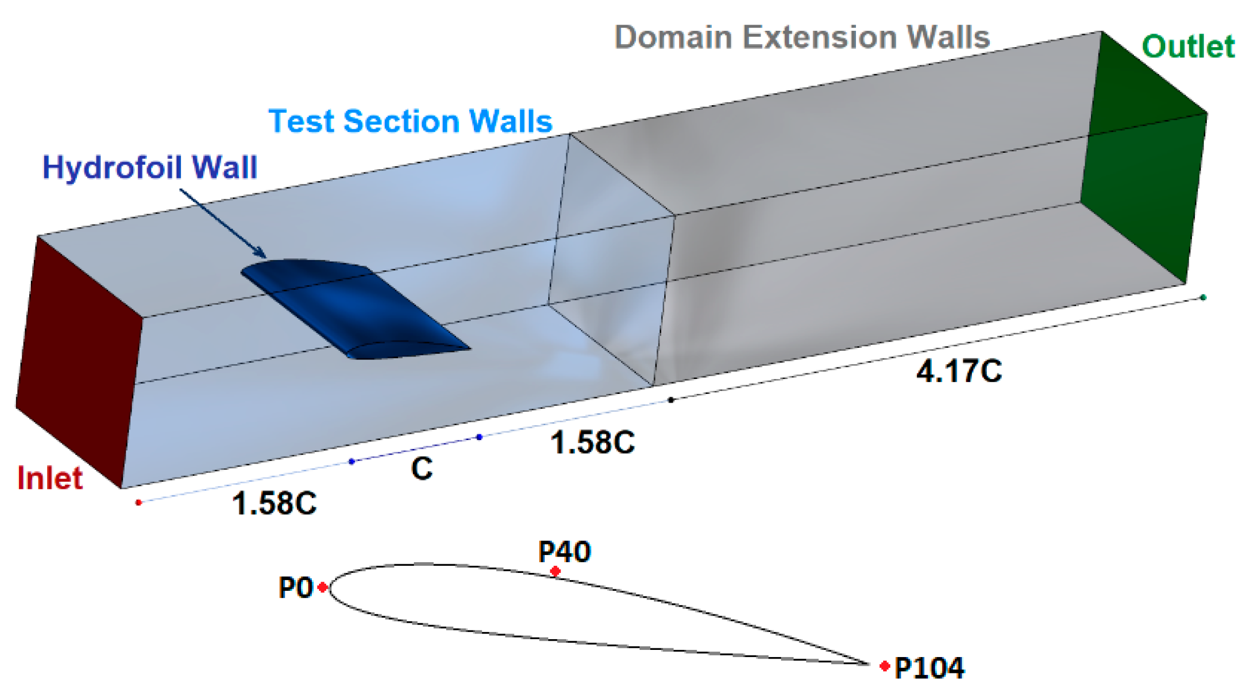
3.1. Hot Water Test Case Setup

The cavitation tunnel test section represents a channel 30 × 20 mm in cross-section and 330 mm long (see Figure 1). The cavitation number σ changes in the range from 1.608 up to 3.822. The water velocity at the test section inlet during the experiments was set to 6 m/s. Concerning the Reynolds number based on the mean velocity at the test section inlet U₀, the dimension of the triangle side d and the water kinematic viscosity ν

$$Re=\frac{d{U}_0}{\mathsf{\nu }},$$

(3)

reaches the value of 1.437 × 10⁵.

Two thermistor probes measured simultaneously the freestream temperature and temperature in the cavitation region behind the cylinder. The temperature depression in the measurement point located inside the cavitation region reached up to 0.225 K. Le and Iga also presented a numerical simulation for one cavitation number to validate their simplified thermodynamics model. Simplified 2D grid with O-grid topology was used with moderate mesh size (241 × 180). The laminar flow and the Wilcox k-ω turbulence model were applied for the viscosity.

In our study, the structured computational grid which respects the 3D tunnel test section geometry (Figure 2) has approximately 18 million nodes. The computational time step was set to Δt = 1 × 10⁻⁵ s. Four values of the cavitation number were considered for simulations in order to estimate the trends and differences between the numerical and experimental data: 3.416, 2.221, 1.722, and 1.675. Default cavitation model parameters were applied, particularly the inlet nuclei volume fraction 5 × 10⁻⁴, the mean nuclei diameter 2 × 10⁻⁶ m, the empirical cavitation condensation parameter equal to 0.01, and the empirical cavitation vaporization parameter equal to 50.

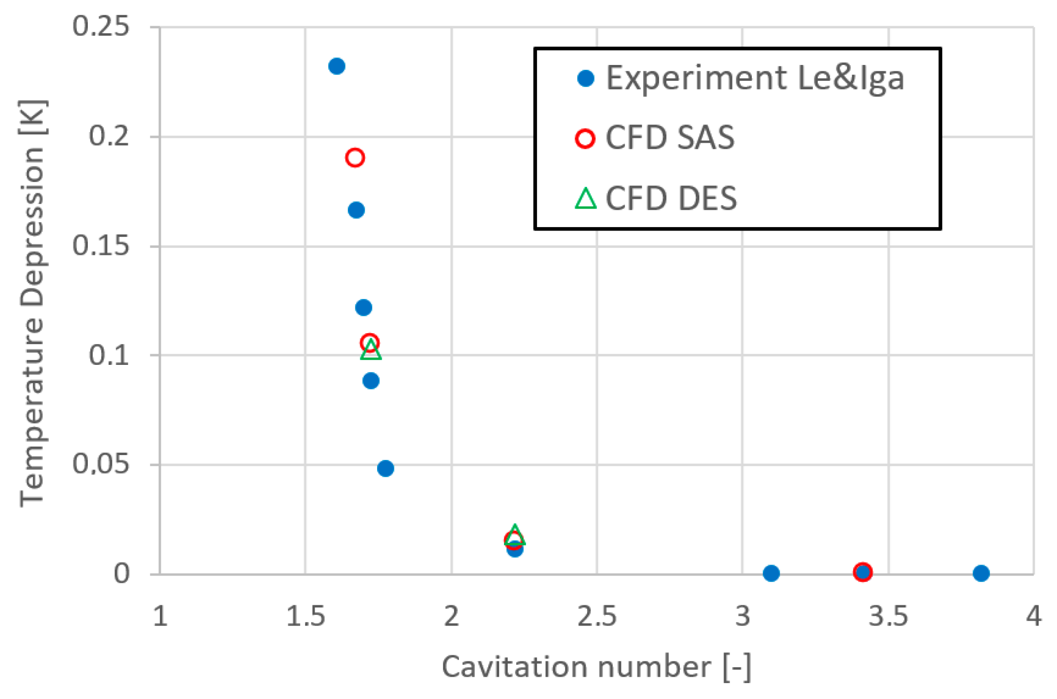
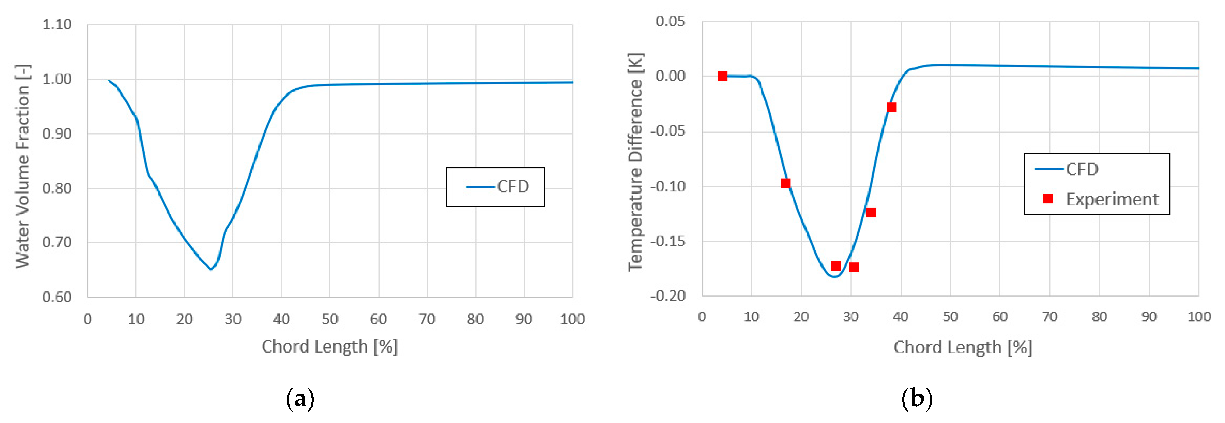
3.2. Hot Water Test Case Results

The results from the SAS and DES models were very similar (as indicated in Figure 3), but the simulations with SAS were more stable and robust; so the main results presented in this study were taken from the SAS simulations, where a larger scope of cavitation numbers were treated. Figure 3 shows the temperature depression at the location of the thermistor 2 (calculated for four different cavitation numbers σ with the SAS turbulence model and for two cavitation numbers σ applying the DES simulations) compared with experiments. With decreasing cavitation number, there is an increasing temperature depression as well as an increasing difference between calculated and experimental data. Still, the relative difference decreases with decreasing cavitation number. There are several reasons for these differences. The first one is the fact that for larger cavitation numbers, a very clear vortex street is formed behind the cylinder, with the low-pressure regions passing periodically close to the position of the thermistor 2. Though the time-averaged temperature depression is very low (0.015 K for σ = 2.221), in fact for some time instants it can reach quite a high value (up to 0.057 K for σ = 2.221), but most of the time it is practically zero. For low cavitation numbers the temperature depression at the location of the thermistor 2 is nearly constant in time with small high-frequency changes resulting from turbulent eddies. However, there is still an influence of the 3D geometry of the tunnel with the side walls. In any case the temperature is not uniform inside the cavity behind the cylinder and its minima and maxima are influenced by the time-developing vortices.

Figure 4 and Figure 5 show vector lines and the distribution of the water volume fraction and water temperature in the test section mid-plane as well as the vortical structures behind the cylinder for the cavitation numbers σ = 2.221 and σ = 1.676. Figure 6 and Figure 7 show the distribution of the water temperature on the cylinder surface and the shape of the cavities behind the cylinder for the same cavitation numbers. Cavitation regions in these figures can be compared with the visualization of the experimental results in Figure 8. The calculated water volume fraction for σ = 1.676 shows a developed cavitation core filled only with vapour, which can be found in the experimental results with the slightly lower cavitation numbers (Figure 8, right).

4. Steady Cavitation Test Case

The hot water test case relied on data obtained from the literature and provided valuable and encouraging results. Nevertheless, some flow conditions were not known, alth ough they can significantly influence the development of the cavitation (e.g., the nuclei size distribution and the nuclei volume fraction). For that reason, the default values of the coefficients were used in the cavitation model. To fit the coefficients of the cavitation model for the new simulations of the partial cavity oscillation on the NACA2412 hydrofoil in the cavitation tunnel including thermal effects, simplified experimental research was performed in this cavitation tunnel with a steady cavitating flow around a hydrofoil used in the past for the cavitation erosion tests [32]. During these previous tests, very low unsteadiness of the cavitating flow was proved with visualizations and with a very narrow strip of pits on the hydrofoil surface, which agrees very well with the numerical simulations and indicates a significant stable location of the first cavitation bubble collapse.

The experimental 2D hydrofoil is equipped with a set of thermistors, which can measure surface temperature at the midspan of the hydrofoil and detect the vaporization and condensation regions.

4.1. Steady Cavitation Test Case Setup

The experimental 2D hydrofoil, sketched in Figure 9, has a chord length of 100 mm and a maximum thickness of 23.5 mm. Its cross-section consists of the 3:2 elliptical nose and the NACA 0020 tail joined at the maximum thickness. The incidence angle of the hydrofoil is set to −1°. The hydrofoil is equipped with a holder containing six thermistor probes on the upper side. The holder is made by 3D printing from co-polyester material and the gaps around the thermistor probes are filled with the Loctite glue and carefully polished (Figure 10a). The temperature measurement uncertainty is 0.01 K.

The cavitation tunnel (Figure 10b) represents a closed, horizontally situated water tunnel with the test section adapted for isolated hydrofoils. The capacity of the main tank is 35 m³. It is equipped with both a compressor and vacuum pump which enable different pressure levels to be set independently of the volume flow rate. The inner dimensions of the rectangular test section are 150 × 150 × 500 mm. For measurement of the volume flow rate a magnetic-inductive flowmeter of accuracy class of 0.3% was used. All static pressures (at the tunnel confusor inlet, diffuser outlet and the test section inlet and outlet) are measured by the transducers with accuracy class 0.1%. The temperature of the water is measured by a platinum thermometer located in the tank, with the class of accuracy 0.5%. ABS acoustic bubble spectrometer can be periodically used to monitor the cavitation nuclei in the inlet flow. The Reynolds number (based on the test section inlet velocity and the hydrofoil chord length) was set to 1.7 × 10⁶. To avoid the unsteady cavitation regime, two relatively high values of the cavitation number (based on the test section inlet static pressure and velocity) were considered: 1.9 and 1.83.

Concerning the CFD setup, the structured computational grid corresponding to the 3D tunnel test section geometry has approximately 17 million nodes. Because of very low unsteadiness of the cavitating flow, the computational time step was set to Δt = 1 × 10⁻³ s, which enables attainment of local Courant numbers below the value of 5 (the limit recommended for the ANSYS CFX solver [26]). The inlet cavitation nuclei volume fraction was set (based on the measurements with the acoustic bubble spectrometer) to 1 × 10⁻⁴. Unfortunately, the cavitation model used enables employment of only one reference initial size of the nuclei. It works correctly only with very small initial nuclei diameters. As shown in [32], the relative growth of these nuclei is much larger than that of the bigger nuclei. For that reason, the mean nuclei diameter was set to default value 2 × 10⁻⁶ m, though the measured nuclei radii reach up to 0.1 mm. The empirical cavitation condensation and cavitation vaporization parameters were modified, as discussed in the next section.

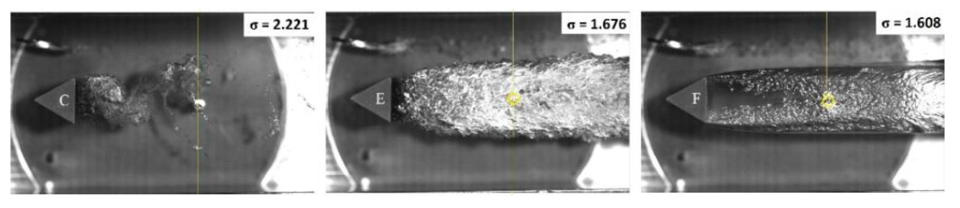
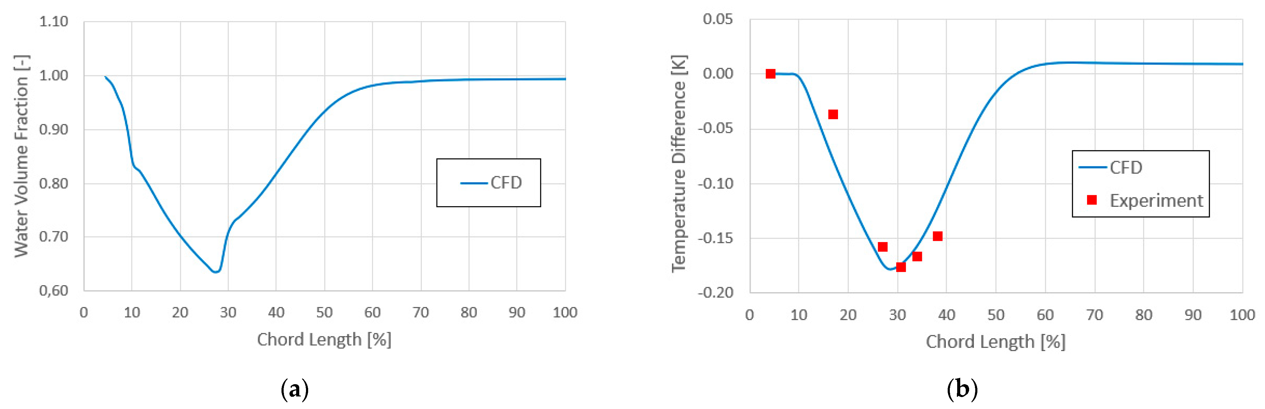
4.2. Steady Cavitation Test Case Results

The first experiments and numerical simulations were performed for the cavitation number σ = 1.9, aiming to adjust the empirical cavitation condensation and cavitation vaporization constants. With this cavitation number, the whole of the cavity is located between the first and the last thermistor probe and both the calculated drop and the recovery of the temperature could be compared with the experimental data measured at midspan of the hydrofoil. Based on these comparisons, the empirical cavitation vaporization parameter was set to the value of 35 and the empirical condensation parameter set to the value of 0.006. Figure 11a shows the calculated distribution of the water volume fraction on the upper side of hydrofoil along the cord length, while Figure 11b shows the comparison of the calculated and measured temperature difference related to the first thermistor probe.

To verify the adjusted empirical cavitation parameters, the other experiments and numerical simulations were conducted for the cavitation number σ = 1.83. With this cavitation number, the cavity is located behind the first thermistor probe but extends to the last probe as shown in Figure 12. The agreement seems to be satisfactory.

Figure 13, Figure 14, Figure 15 and Figure 16 show the calculated distribution of the water volume fraction and temperature difference on the upper side of hydrofoil as well as 3D views of the cavitation, evaporation, and condensation regions for both cavitation numbers. The cavitation regions are visualized by means of the iso-surfaces of water volume fraction 90%. These cavitation regions can be compared with the visualizations from experiments in Figure 17.

5. Partial Cavity Oscillation on the Hydrofoil

The main goal of this study was a numerical analysis of highly unsteady partial cavity oscillation on hydrofoils. The straight NACA2412 hydrofoil with a chord length of 120 mm and a span of 150 mm (giving the span/chord ratio of 1.25) was experimentally tested in the same cavitation tunnel as described in Section 4.1.

5.1. Case Description

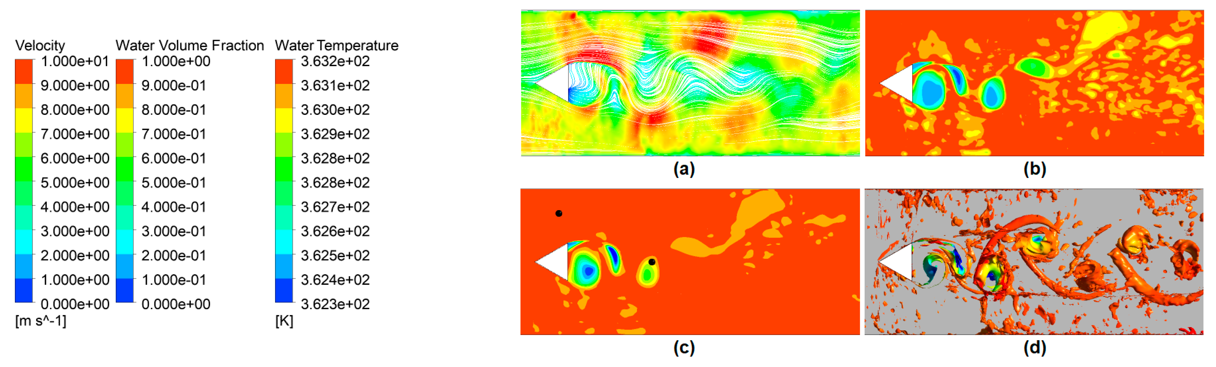
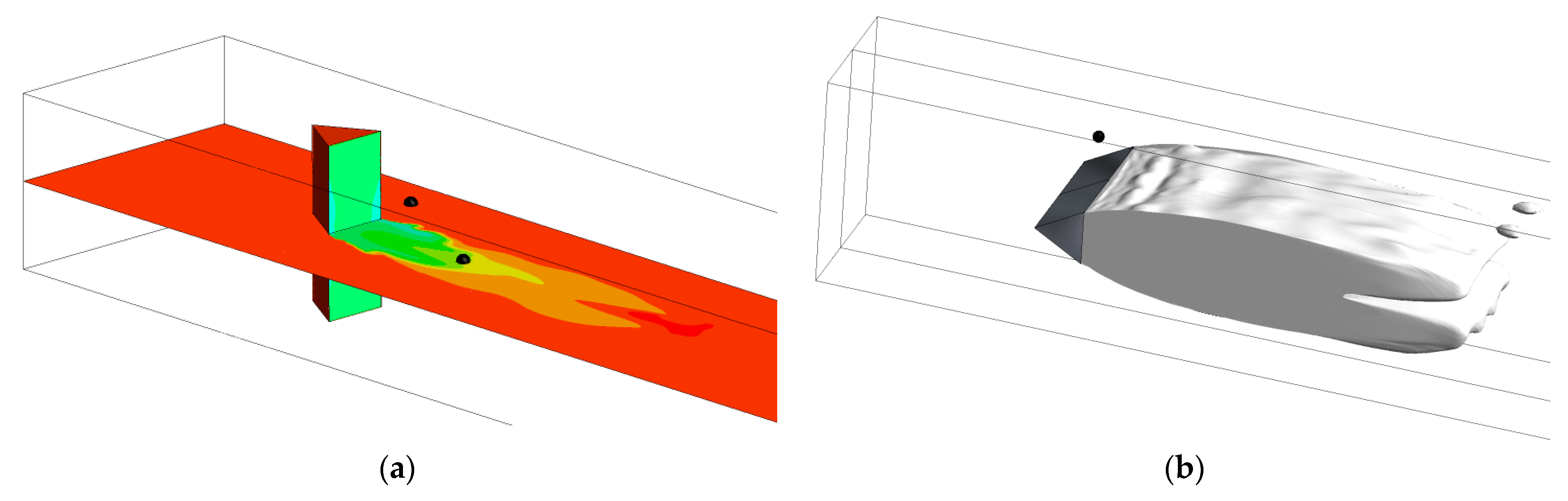
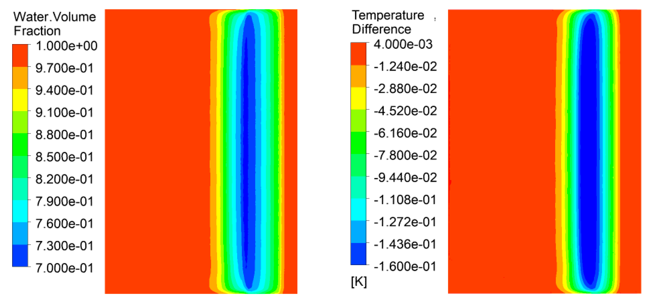
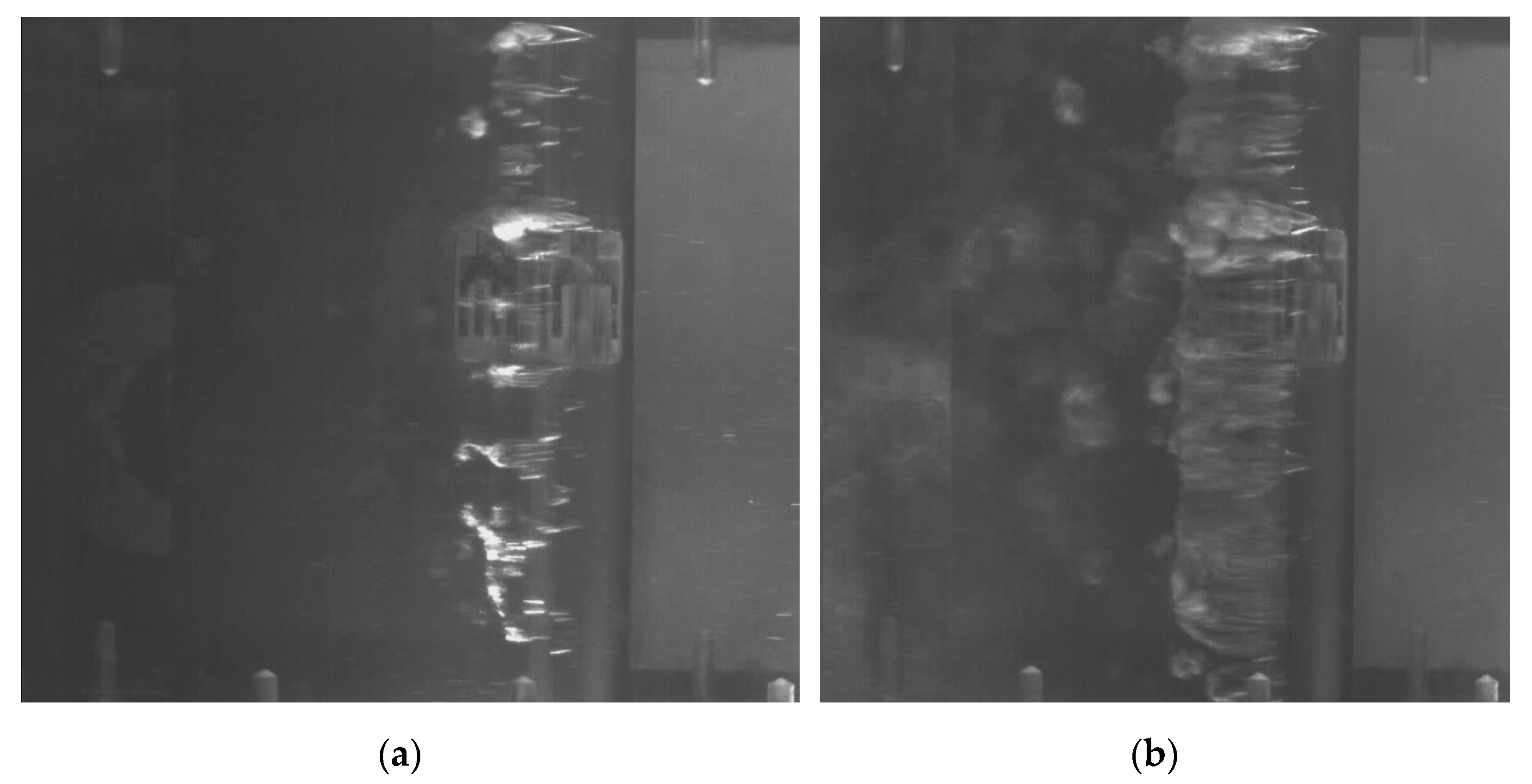
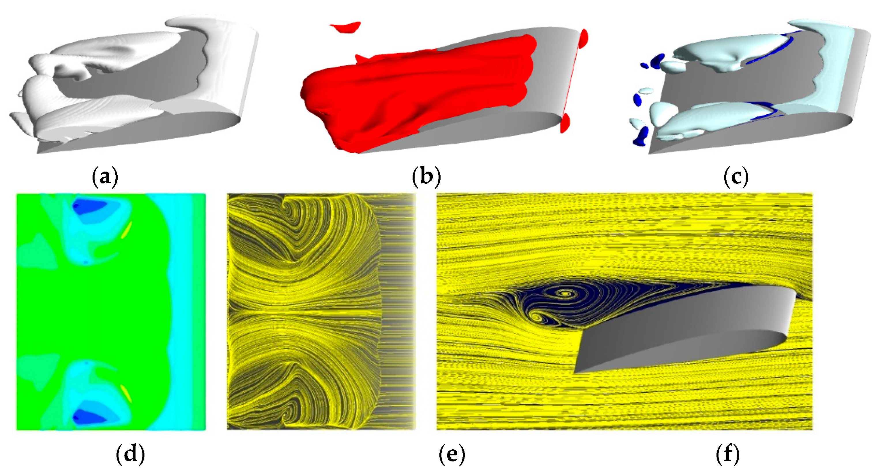
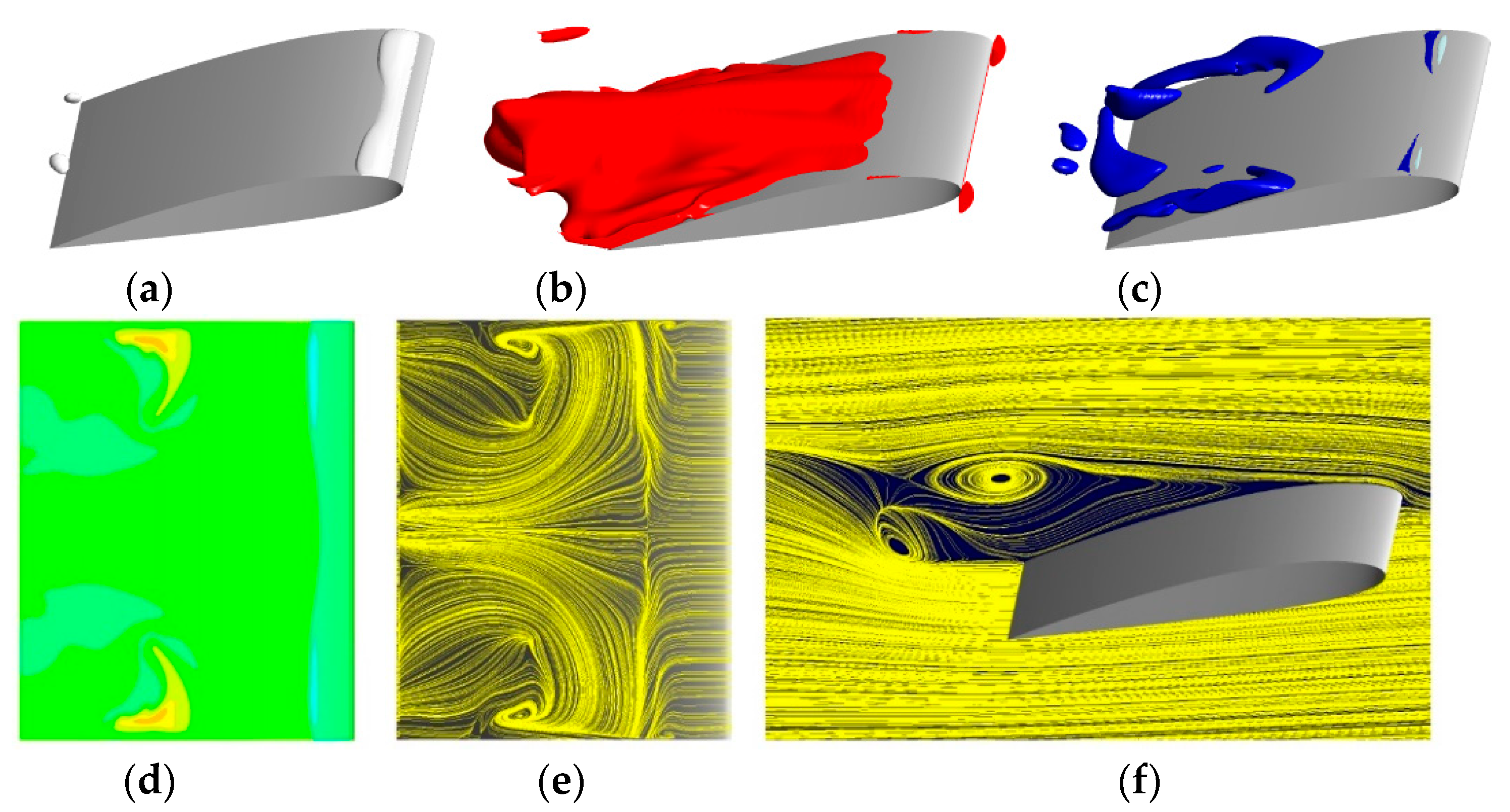
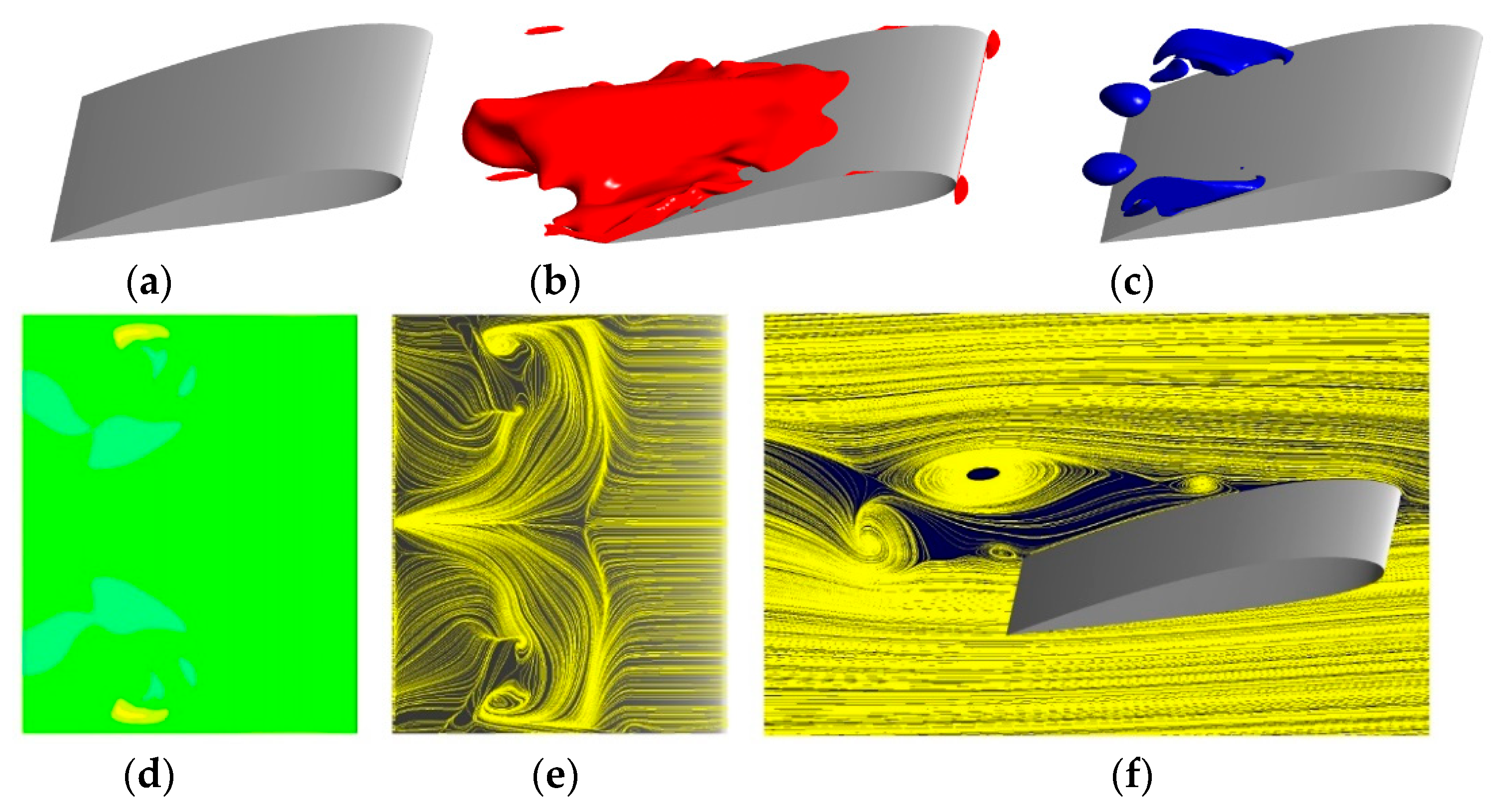
Similar to the steady cavitation test case, the computational domain corresponds to the rectangular tunnel test section with inner dimensions 150 × 150 × 500 mm (Figure 18). The tested NACA2412 hydrofoil has the incidence angle of 8°, which enables the fully periodic regime of the partial cavity oscillation to be achieved. The hydrofoil was equipped with two pressure transducers at the symmetry plane. The first one has a tap hole at the leading edge (pressure P0, see Figure 18 bottom right), the tap hole of the second transducer is located on the suction side (at 40% of the chord length, pressure P40). The high-frequency pressure pulses behind the hydrofoil trailing edge were monitored by the PVDF hydrophone (104% of chord length, P104). The Reynolds number (defined similarly to Section 4.1) was set to 1.56 × 10⁶.

Though the hydrofoil has a two-dimensional character, the full geometry of the tunnel test section was modelled to capture the three-dimensional effects resulting from the presence of side-walls. The computational domain has its length twice as long as the tunnel test section because it was extended so as not to influence the separation regions on the hydrofoil by the outlet boundary condition. The resulting structured computational grid (of the C-type with sharp trailing edge) contains approximately 24 million nodes. As already mentioned, the values of y+ monitored in time remained close to 1 on all the hydrofoil and side walls during the whole shedding cycle.

The uniform velocity, turbulence intensity, and length scale are prescribed at the inlet as the inlet boundary condition. The value of the average static pressure, corresponding to the experimental data, is set at the outlet. According to the tunnel geometry, the inlet boundary is located 1.58 C in front of the foil leading edge. The outlet boundary was placed 5.75 C downstream of the trailing edge. As in the test cases, the initial calculations employed the URANS equations with the standard SST turbulence model and then the SAS-SST and the DES models were used. The computational time step was Δt = 2 × 10⁻⁵ s. All the settings for the cavitation model were taken from Section 4.2.

5.2. Results

The results presented in this section concentrate on the interactions between the re-entrant flow and cavitation regions during the partial cavitation oscillation as well as on the high-pressure pulsations during the collapses of the cavitation clouds after the breakup of the cavity on the hydrofoil suction side. These results come from the SAS-SST simulations. As shown in [7], for quite a narrow range of the cavitation numbers σ (approximately from 1.3 to 2) experimental results indicate the appearance of the “resonance” regime, in which very regular partial cavity oscillation appears with the pressure pulses reaching high values, with a distinct maximum about 400 kPa at σ_resonant = 1.71. That is why this value of the cavitation number was used for the presented numerical simulations. Both the measured and calculated dominant frequency of the partial cavity oscillation at σ_resonant is about 15 Hz. The left hand side of Figure 19 shows normalized amplitudes of pressure pulses at position P40 measured for 21 cavitation numbers. The right hand side of Figure 19 shows the pressure pulse calculated during one typical shedding cycle. The red control points 1–8 are marked for future visualizations.

The simulations presented in [8] confirm, that the physical models based on the incompressible constant property liquids overpredict significantly the maxima of the pressure peaks as well as the speed of their propagation. The maximum pressure pulses obtained from the numerical simulations reached up to 800 kPa compared with the experimental results, which did not exceed 400 kPa. That is why our attention was concentrated on the improvement of the CFD accuracy by describing the real properties of water, respecting the assessed content of undissolved air, and modelling the thermal effects of cavitation, which can play a significant role.

Figure 20, Figure 21, Figure 22, Figure 23, Figure 24, Figure 25, Figure 26, Figure 27 and Figure 28 (top) show the 3D view of the cavitation regions, back-flow regions and evaporation and condensation regions. At the bottom of the figures, there are pictures of the temperature differences with vector lines on the hydrofoil suction surface and vector lines at the midspan of the hydrofoil. The cavitation regions are represented by the iso-surfaces on which the local void fraction reaches 10%. The backflow regions are depicted as the regions with a negative longitudinal velocity. The time instants 1–8 correspond to the graph in Figure 19b. The first time instant (Figure 21) is characterized by large evaporation regions with decreased temperature and very small condensation regions with increased temperature. The cavitation region is split into two main parts, with the remnant of the sheet cavity behind the leading edge and cavitation clouds in the rear part of the hydrofoil. During the next two instants (Figure 22 and Figure 23) the condensation regions decrease, especially in the rear part of the hydrofoil and completely disappear in the fourth time instant (Figure 24). This phenomenon is accompanied by complete vanishing of the cavitation region on the hydrofoil while the maximum static pressure reached 40% of the hydrofoil chord length. In the next time instants (Figure 25, Figure 26 and Figure 27) a new sheet cavity is formed behind the leading edge and accompanied by the evaporation region. During time instants 5 and 6, the backflow region decreases and its leading edge moves towards the hydrofoil trailing edge. In time instant 7, the new re-entrant flow forms in the central part of the hydrofoil suction side. It starts to grow (with its leading edge moving towards the hydrofoil leading edge) and interacts with the rear part of the cavity. Consequently, the sheet cavity loses its stability and starts to split, as shown in Figure 28.

As has been already said, in the simulations which do not respect the real properties of liquid media and thermal effects of cavitation [8], the sharp high-pressure peaks corresponding to the time instant 4 in Figure 19b were overpredicted up to two times. Moreover, the pressure peaks in positions P0, P40, and P104 were obtained at the same time and had nearly the same amplitude, which indicates that the speed of pressure pulse propagation is highly overpredicted. Figure 29b shows the pressure pulse calculated in positions P0 and P40 when considering the real properties of fluid, compared to the experimental data. The amplitude of the pulse in the position P0 close to the leading edge is significantly lower than the amplitude at 40% of the chord length. Moreover, there is also a time shift in between the pulse peaks in these two positions, which corresponds well with the measurements shown in Figure 29a.

6. Discussion

The numerical simulations presented in Section 5 confirm, that the CFD tools are able to capture very dynamic cavitation structures, including the ones resulting from the cavitation instabilities on the hydrofoils or blades of hydraulic machines. One of the most important examples is the partial cavity oscillation on the blades of hydraulic machines which is connected with high-pressure pulses and increased vibrations and noise. When respecting the real properties of liquid media, the numerical tools can also predict the magnitudes of the high-pressure peaks and the speed of their propagation in a realistic way. Figure 30 shows aerodynamic loads calculated during one shedding cycle. It can be seen that besides a relatively smooth periodic course (but with appreciable differences between minima and maxima), the high-pressure pulse causes an abrupt change of the forces and torque acting on the hydrofoil, which can result in dangerous vibrations. To estimate correctly these abrupt effects, the improved model of the pressure propagation seems to be essential.

On considering the Mach numbers in our simulations, under non-cavitating (wet) flow, they do not exceed the value of 0.1. Of course, inside the cavitation regions, the local Mach number in the water-vapour mixture can be even much lower than the Mach number inside the pure vapour. As the content inside the cavitation regions is not in reality a real continuum and contains interacting cavitation bubbles, it is practically impossible to estimate the local Mach number correctly. The graphs in Figure 29 and Figure 30 indicate, that the propagation speed of the high-pressure pulse is in the magnitude of tens of metres per second. This is more realistic than the propagation speeds in thousands of metres per second, resulting from the simulations, which do not respect the real properties of liquid media and the thermal effects of cavitation. From this point of view, it could be concluded, that in macroscale, the cavitating flow remains subsonic, though in microscale, shock waves can appear inside the collapsing cavitation structures.

Normally, the physical properties of water and steam can be described by the IAPWS IF97 formulation [33]. However, during the convergence process (especially at its beginning) the CFD solver returns physically invalid values (e.g., large negative values of pressure or enthalpy), which cannot be treated by IF97 formulation. So, both the water and the water vapour should be described by the RGP tables, which would cover a wide range of unexpected physical states. The undissolved air at the water with estimated volume fraction of 0.1% can be treated as an ideal gas.

Besides the real properties of liquid media, the thermal effects of cavitation can play a significant role, although these are normally considered only for cryogenic fluids or high temperature water. In this study, the conservation equation of temperature for the mixture phase is based on the mixture total energy conservation equation.

To verify the calculation of the thermodynamic effect on cavitation, the experimental data from Le and Iga [31] were used. The numerical simulations showed that the temperature depression inside the cavitation region strongly depends on the cavitation number (cavitation intensity) and that the accuracy of the measurements (as well as the agreement of numerical simulations and experiments) decreases with increasing cavitation flow unsteadiness. Because it was not able to use thermistor probes with sufficient recording frequency of several hundred hertz for the partial cavitation oscillation on the NACA2412 hydrofoil, the simplified experimental research was performed with steady cavitating flow around a modified NACA0020 hydrofoil in the same cavitation tunnel. The aim was to calibrate the cavitation model only for the cavitation tunnel operated in the Centre of Hydraulic Research. Good agreement of numerical simulations and experiments was achieved. Nevertheless, it is not possible to generalize the obtained empirical cavitation coefficients for the simulations under completely different experimental conditions and different temperature ranges. Usually, different water cavitation tunnels show slightly different results, even for experiments with the same geometries, sizes, and dimensionless reference numbers because the cavitation phenomena depend on many parameters including the quality of water and the cavitation nuclei content. On the other hand, this study assumed, that the cavitation simulation parameters obtained with the steady simulations could be used for the unsteady ones in the same cavitation tunnel and under the same conditions without a significant decrease of reliability.

Two advanced turbulence models including the SAS-SST and DES ones were used for the numerical simulations. The results from the SAS and DES models do not differ substantially but the simulations with SAS were more stable and robust; thus, the results presented are taken from the SAS simulations, where a much larger number of shedding cycles could be obtained. Still, simulations show that for both advanced turbulence models, the physical model based on the real properties of water and vapour was determinative for the possibility of the propagation of the pressure pulses and their amplitudes to be well estimated.

To compare the requirements of the CFD models based on the real properties of water including the estimated content of undissolved air and the models based on the incompressible constant property fluids, the former require approximately double computational times (valid for the used CFD code ANSYS CFX).

References

1. Tsujimoto, Y. Cavitation Instabilities in Turbopump Inducers. In Fluid Dynamics of Cavitation and Cavitating Turbopumps, 2007th ed.; d’Agostino, L., Salvetti, M.V., Eds.; Springer, Wien: New York, NY, USA, 2007; pp. 169–190. [Google Scholar]
2. Tsujimoto, Y.; Watanabe, S.; Horiguchi, H. Cavitation Instabilities of Hydrofoils and Cascades. Int. J. Fluid Mach. Syst. 2008, 1, 38–46. [Google Scholar] [CrossRef]
3. E Brennen, C. A review of the dynamics of cavitating pumps. IOP Conf. Ser. Earth Environ. Sci. 2012, 15, 012001. [Google Scholar] [CrossRef]
4. Kobayashi, K.; Chiba, Y. Computational Fluid Dynamics of Cavitating Flow in Mixed Flow Pump with Closed Type Impeller. Int. J. Fluid Mach. Syst. 2010, 3, 113–121. [Google Scholar] [CrossRef]
5. Sedlar, M.; Sputa, O.; Komarek, M. CFD Analysis of Cavitation Phenomena in Mixed-Flow Pump. Int. J. Fluid Mach. Syst. 2012, 5, 18–29. [Google Scholar] [CrossRef]
6. Reisman, G.E.; Brennen, C.E. Shock wave measurements in cloud cavitation. In Proceedings of the 21st International Symposium on Shock Waves, Great Keppel Island, Australia, 20–25 July 1997; p. 1570. [Google Scholar]
7. Sedlář, M.; Komárek, M.; Rudolf, P.; Kozák, J.; Huzlik, R. Numerical and experimental research on unsteady cavitating flow around NACA 2412 hydrofoil. IOP Conf. Ser. Mater. Sci. Eng. 2015, 72, 022014. [Google Scholar] [CrossRef]
8. Sedlar, M.; Ji, B.; Kratky, T.; Rebok, T.; Huzlik, R. Numerical and experimental investigation of three-dimensional cavitating flow around the straight NACA2412 hydrofoil. Ocean Eng. 2016, 123, 357–382. [Google Scholar] [CrossRef]
9. Yamaguchi, Y.; Iga, Y. Thermodynamic Effect on Cavitation in High Temperature Water. In Proceedings of the Fluids Engineering Division Summer Meeting, Chicago, IL, USA, 3–7 August 2014. [Google Scholar] [CrossRef]
10. Petkovšek, M.; Dular, M. Experimental study of the thermodynamic effect in a cavitating flow on a simple Venturi geometry. J. Phys. Conf. Ser. 2015, 656, 012179. [Google Scholar] [CrossRef]
11. Cervone, A.; Bramanti, C.; Rapposelli, E.; d’Agostino, L. Thermal Cavitation Experiments on a NACA 0015 Hydrofoil. J. Fluids Eng. 2006, 128, 326–331. [Google Scholar] [CrossRef]
12. Iga, Y.; Furusawa, T.; Sasaki, H. Interaction Between Thermodynamic Suppression Effect and Reynolds Number Promotion Effect on Cavitation in Hot Water; ASME Press: New York, NY, USA, 2018; pp. 576–580. [Google Scholar] [CrossRef] [Green Version]
13. Zhang, H.; Zuo, Z.; Mørch, K.A.; Liu, S. Thermodynamic effects on Venturi cavitation characteristics. Phys. Fluids 2019, 31, 097107. [Google Scholar] [CrossRef]
14. Niiyama, K.; Yoshida, Y.; Hasegawa, S.; Watanabe, M.; Oike, M. Experimental Investigation of Thermodynamic Effect on Cavitation in Liquid Nitrogen. In Proceedings of the 8th International Symposium on Cavitation, Singapore, 13–16 August 2012; pp. 153–157. [Google Scholar] [CrossRef]
15. Zhu, J.; Xie, H.; Feng, K.; Zhang, X.; Si, M. Unsteady cavitation characteristics of liquid nitrogen flows through venturi tube. Int. J. Heat Mass Transf. 2017, 112, 544–552. [Google Scholar] [CrossRef]
16. Tsuda, S.-I.; Watanabe, S. CFD Simulation of Thermodynamic Effect Using a Homogeneous Cavitation Model Based on Method of Moments; ASME Press: New York, NY, USA, 2018; pp. 249–252. [Google Scholar] [CrossRef]
17. Franc, J.-P.; Pellone, C. Analysis of Thermal Effects in a Cavitating Inducer Using Rayleigh Equation. J. Fluids Eng. 2007, 129, 974–983. [Google Scholar] [CrossRef]
18. Chen, T.R.; Wang, G.Y.; Huang, B.; Li, D.Q.; Ma, X.J.; Li, X.L. Effects of physical properties on thermo-fluids cavitating flows. J. Phys. Conf. Ser. 2015, 656, 012181. [Google Scholar] [CrossRef]
19. Wang, S.; Zhu, J.; Xie, H.; Zhang, F.; Zhang, X. Studies on thermal effects of cavitation in LN2 flow over a twisted hydrofoil based on large eddy simulation. Cryogenics 2019, 97, 40–49. [Google Scholar] [CrossRef]
20. Shi, S.; Wang, G. Thermal Effects on Cryogenic Cavitating Flows around an Axisymmetric Ogive. Int. J. Fluid Mach. Syst. 2010, 3, 324–331. [Google Scholar] [CrossRef]
21. Liang, W.; Chen, T.; Huang, B.; Wang, G. Thermodynamic analysis of unsteady cavitation dynamics in liquid hydrogen. Int. J. Heat Mass Transf. 2019, 142, 118470. [Google Scholar] [CrossRef]
22. Viitanen, V.M.; Sipilä, T.; Sánchez-Caja, A.; Siikonen, T. Compressible Two-Phase Viscous Flow Investigations of Cavitation Dynamics for the ITTC Standard Cavitator. Appl. Sci. 2020, 10, 6985. [Google Scholar] [CrossRef]
23. Ghahramani, E.; Ström, H.; Bensow, R. Numerical simulation and analysis of multi-scale cavitating flows. J. Fluid Mech. 2021, 922, A22. [Google Scholar] [CrossRef]
24. Zhang, H.; Zuo, Z.; Liu, S. Influence of Dissolved Gas Content on Venturi Cavitation at Thermally Sensitive Conditions; ASME Press: New York, NY, USA, 2018; pp. 546–550. [Google Scholar] [CrossRef]
25. Brandao, F.; Bhatt, M.; Mahesh, K. Effects of Non-Condensable Gas on Cavitating Flow Over a Cylinder. In Proceedings of the 10th International Symposium on Cavitation, Baltimore, MD, USA, 14–16 May 2018; pp. 346–351. [Google Scholar] [CrossRef]
26. ANSYS CFX-Solver Theory Guide Release 2020 R1—©; ANSYS, Inc.: Canonsburg, PA, USA, 2020.
27. Zwart, P.J.; Gerber, A.G.; Belamri, T. A Two-Phase Flow Model for Predicting Cavitation Dynamics. In Proceedings of the Fifth International Conference on Multiphase Flow, Yokohama, Japan, 30 May 2004; Volume 152. [Google Scholar]
28. Menter, F.; Egorov, Y. A Scale Adaptive Simulation Model using Two-Equation Models. In Proceedings of the 43rd AIAA Aerospace Sciences Meeting and Exhibit, Reno, NV, USA, 10–13 January 2005. [Google Scholar] [CrossRef]
29. Menter, F.; Kuntz, M.; Bender, R. A Scale-Adaptive Simulation Model for Turbulent Flow Predictions. In Proceedings of the 41st Aerospace Sciences Meeting and Exhibit, Reno, NV, USA, 6–9 January 2003. [Google Scholar] [CrossRef]
30. Menter, F.; Schütze, J.; Kurbatskii, K.; Lechner, R.; Gritskevich, M.S.; Garbaruk, A. Scale-Resolving Simulation Techniques in Industrial CFD. In Proceedings of the 6th AIAA Theoretical Fluid Mechanics Conference, Honolulu, HI, USA, 27–30 June 2011; pp. 2011–3474. [Google Scholar]
31. Le, A.D.; Iga, Y. A simplified thermodynamic effect model for cavitating flow in hot water. IOP Conf. Ser. Earth Environ. Sci. 2019, 240, 062024. [Google Scholar] [CrossRef]
32. Sedlář, M.; Komárek, M.; Vyroubal, M.; Muller, M. Experimental and numerical analysis of cavitating flow around a hydrofoil. EPJ Web Conf. 2012, 25, 01084. [Google Scholar] [CrossRef]
33. Wagner, W.; Cooper, J.R.; Dittmann, A.; Kijima, J.; Kretzschmar, H.-J.; Kruse, A.; Mareš, R.; Oguchi, K.; Sato, H.; Stöcker, I.; et al. The IAPWS Industrial Formulation 1997 for the Thermodynamic Properties of Water and Steam. ASME J. Eng. Gas Turbines Power 2000, 122, 150–184. [Google Scholar] [CrossRef]
Figure 1. Overview of cavitation tunnel test section and thermistor probes. Credit: Le and Iga [31].
Energies 15 06503 g001
Figure 2. Topology of computational domain. Black balls indicate position of thermistor probes.
Energies 15 06503 g002
Figure 3. Comparison of CFD results with experimental data by Le and Iga [31].
Energies 15 06503 g003
Figure 4. Cavitation at test section mid-plane, σ = 2.221. (a) Vector lines; (b) distribution of water volume fraction; (c) distribution of temperature; (d) vortical structures behind the cylinder (Q criterion) colored with temperature.
Energies 15 06503 g004
Figure 5. Cavitation at test section mid-plane, σ = 1.676. (a) Vector lines; (b) distribution f water volume fraction; (c) distribution of temperature; (d) vortical structures behind the cylinder (Q criterion) colored with temperature.
Energies 15 06503 g005
Figure 6. 3D view, σ = 2.221. (a) Distribution of temperature on cylinder surface and at test section mid-plane; (b) shape of cavities behind cylinder.
Energies 15 06503 g006
Figure 7. 3D view, σ = 1.676. (a) Distribution of temperature on cylinder surface and at test section mid-plane; (b) shape of cavities behind cylinder.
Energies 15 06503 g007
Figure 8. Visualization of cavitation structures in cavitation tunnel. Credit: Le and Iga [31].
Energies 15 06503 g008
Figure 9. (a) 3D view of hydrofoil with thermistor holder; (b) cross-section of hydrofoil with thermistors 1–6.
Energies 15 06503 g009
Figure 10. (a) Thermistor probes on upper side of hydrofoil; (b) picture of cavitation tunnel test section.
Energies 15 06503 g010
Figure 11. Comparison of numerical and experimental results on upper side of hydrofoil, σ = 1.9. (a) Distribution of water volume fraction; (b) temperature difference related to the first thermistor probe position.
Energies 15 06503 g011
Figure 12. Comparison of numerical and experimental results on upper side of hydrofoil, σ = 1.83. (a) Distribution of water volume fraction; (b) temperature difference related to the first thermistor probe position.
Energies 15 06503 g012
Figure 13. Distribution of water volume fraction and temperature difference on upper side of hydrofoil, σ = 1.9. CFD.
Energies 15 06503 g013
Figure 14. 3D view of cavitation at σ = 1.9. (a) Iso-surface of water volume fraction 90%. Red balls indicate positions of thermistor probes; (b) evaporation regions (in light cyan) and condensation regions (in dark blue). CFD.
Energies 15 06503 g014
Figure 15. Distribution of water volume fraction and temperature difference on upper side of hydrofoil, σ = 1.83. CFD.
Energies 15 06503 g015
Figure 16. 3D view of cavitation at σ = 1.83. (a) Iso-surface of water volume fraction 90%. Red balls indicate positions of thermistor probes; (b) evaporation regions (in light cyan) and condensation regions (in dark blue). CFD.
Energies 15 06503 g016
Figure 17. 3D Cavitation on upper side of hydrofoil. Experiment. (a) σ = 1.9; (b) σ = 1.83.
Energies 15 06503 g017
Figure 18. Computational domain and description of boundary conditions (top left) and position of pressure transducers at the symmetry plane (bottom right).
Energies 15 06503 g018
Figure 19. (a) Normalized amplitudes of pressure pulses measured at midspan of hydrofoil at 40% chord length; (b) pressure pulse calculated during one typical shedding cycle and scheme of control points.
Energies 15 06503 g019
Figure 20. (a) Scale of temperature differences on suction side of hydrofoil in Figure 21, Figure 22, Figure 23, Figure 24, Figure 25, Figure 26, Figure 27 and Figure 28; (b) hydrofoil symmetry plane in which vector lines are drawn in Figure 21, Figure 22, Figure 23, Figure 24, Figure 25, Figure 26, Figure 27 and Figure 28.
Energies 15 06503 g020
Figure 21. Time instant 1. (a) 3D view of cavitation regions (in white); (b) Back-flow regions (in red); (c) evaporation regions (in light cyan) and condensation regions (in dark blue); (d) temperature differences on hydrofoil suction side; (e) vector lines on hydrofoil suction side; (f) vector lines in symmetry plane.
Energies 15 06503 g021
Figure 22. Time instant 2. (a) 3D view of cavitation regions (in white); (b) back-flow regions (in red); (c) evaporation regions (in light cyan) and condensation regions (in dark blue); (d) temperature differences on hydrofoil suction side; (e) vector lines on hydrofoil suction side; (f) vector lines in symmetry plane.
Energies 15 06503 g022
Figure 23. Time instant 3. (a) 3D view of cavitation regions (in white); (b) back-flow regions (in red); (c) evaporation regions (in light cyan) and condensation regions (in dark blue); (d) temperature differences on hydrofoil suction side; (e) vector lines on hydrofoil suction side; (f) vector lines in symmetry plane.
Energies 15 06503 g023
Figure 24. Time instant 4. (a) 3D view of cavitation regions (in white); (b) back-flow regions (in red); (c) evaporation regions (in light cyan) and condensation regions (in dark blue); (d) temperature differences on hydrofoil suction side; (e) vector lines on hydrofoil suction side; (f) vector lines in symmetry plane.
Energies 15 06503 g024
Figure 25. Time instant 5. (a) 3D view of cavitation regions (in white); (b) back-flow regions (in red); (c) evaporation regions (in light cyan) and condensation regions (in dark blue); (d) temperature differences on hydrofoil suction side; (e) vector lines on hydrofoil suction side; (f) vector lines in symmetry plane.
Energies 15 06503 g025
Figure 26. Time instant 6. (a) 3D view of cavitation regions (in white); (b) back-flow regions (in red); (c) evaporation regions (in light cyan) and condensation regions (in dark blue); (d) temperature differences on hydrofoil suction side; (e) vector lines on hydrofoil suction side; (f) vector lines in symmetry plane.
Energies 15 06503 g026
Figure 27. Time instant 7. (a) 3D view of cavitation regions (in white); (b) back-flow regions (in red); (c) evaporation regions (in light cyan) and condensation regions (in dark blue); (d) temperature differences on hydrofoil suction side; (e) vector lines on hydrofoil suction side; (f) vector lines in symmetry plane.
Energies 15 06503 g027
Figure 28. Time instant 8. (a) 3D view of cavitation regions (in white); (b) back-flow regions (in red); (c) evaporation regions (in light cyan) and condensation regions (in dark blue); (d) temperature differences on hydrofoil suction side; (e) vector lines on hydrofoil suction side; (f) vector lines in symmetry plane.
Energies 15 06503 g028
Figure 29. Pressure pulse during one shedding cycle in positions P0 and P40. (a) Experiment; (b) numerical simulation employing real properties of fluids.
Energies 15 06503 g029
Figure 30. Aerodynamic loads calculated during one shedding cycle. (a) Drag and lift; (b) torque (axis at hydrofoil maximum thickness). Values of drag are increased ten times for better differentiation.
Energies 15 06503 g030
Publisher’s Note: MDPI stays neutral with regard to jurisdictional claims in published maps and institutional affiliations.