Probabilistic Description of the State of Charge of Batteries Used for Primary Frequency Regulation

Abstract

Battery participation in the service of power system frequency regulation is universally recognized as a viable means for counteracting the dramatic impact of the increasing utilization of renewable energy sources. One of the most complex aspects, in both the planning and operation stage, is the adequate characterization of the dynamic variation of the state of charge of the battery in view of lifetime preservation as well as the adequate participation in the regulation task. Since the power system frequency, which is the input of the battery regulation service, is inherently of a stochastic nature, it is easy to argue that the most proper methodology for addressing this complex issue is that of the theory of stochastic processes. In the first part of the paper, a preliminary characterization of the power system frequency is presented by showing that with an optimal degree of approximation it can be regarded as an Ornstein–Uhlenbeck process. Some considerations for guaranteeing desirable performances of the control strategy are performed by assuming that the battery-regulating power depending on the frequency can be described by means of a Wiener process. In the second part of the paper, more realistically, the regulating power due to power system changes is described as an Ornstein–Uhlenbeck or an exponential shot noise process driven by a homogeneous Poisson process depending on the frequency response features requested of the battery. Because of that, the battery state of charge is modeled as the output of a dynamic filter having this exponential shot noise process as input and its characterization constitutes the central role for the correct characterization of the battery life. Numerical simulations are carried out for demonstrating the goodness and the applicability of the proposed probabilistic approach.

1. Introduction

The problem of continuously and instantaneously balancing generation and load is the most important requirement in power system operation. Traditionally, this service has been performed by power plants of high-rated active power (in Italy, for instance, by those whose rated power is greater than 10 MW) [1]. With the integration of renewable source generators which have priority dispatch, the assurance of stability of the power system is even more critical due to the intermittency typical of such systems [2,3]. Storage technologies seem to be ideal candidates for such service thanks to their ability to track rapid fluctuations encountered in power systems and to their relatively high-power capability, thus being even more appropriate than conventional generators. Conventional generators based on fossil fuels are slower to respond to the operator signal and a require higher and redundant frequency reserve compared to storage systems which are able to provide more accurate regulation. Another important aspect is related to the ability of electrical energy storage, unlike conventional power plants, to avoid the emission of greenhouse gases [4]. While there are many technologies which can be considered suitable for such operation, those based on electrochemical conversion, i.e., battery energy storage systems (BESS), seem to be interesting options thanks to their high ramp rates and their reliability [5].

The viability of BESSs for primary frequency regulation depends on a few issues mainly related to their economic feasibility as well as existing regulations. The U.S. has already moved towards the implementation of battery storage, motivated by the increased variable renewable energy due to state renewable portfolio standards, the falling costs of solar photovoltaic power, the increasing retail electricity rates and regulations that value and pay for fast frequency response [4]. Other challenging aspects related to the use of BESSs refer to technical tasks. The most challenging requirements of BESSs in providing primary frequency regulation are in maintaining their state of charge (SoC) at a level which guarantees capacity availability and preserving the battery lifetime. The considered SoC reestablishing strategy, in fact, significantly influences the lifetime of the battery.

In the technical literature, several proposals have been presented for the use of BESSs in primary frequency regulation aimed at preserving the battery life. In [1], a specific control strategy has been proposed where a variable-droop mode is considered, aimed at exploiting the fast response capability of the BESS when SoC is in a good state while working at a minimum when SoC is limited. In [6], a primary frequency modulation control strategy is proposed based on fuzzy control which also considers the SoC state self-recovery of energy storage. A control algorithm with adjustable SoC limits and the application of dissipation resistors is proposed in [7]. In [8], five strategies for delivering the primary frequency regulation and reestablishing the systems’ SoC have been investigated from the battery lifetime perspective. The study in [9] proposes a control system model to simulate the operation of BESS, and the design of a controller whose strategy is based on model predictive control to ensure the optimal operation of the BESS. A frequency predictor based on the Grey model is also designed to improve the performance of the predictive controller. The prediction model involved can predict frequency multiple steps ahead, this information being used in the optimization part of the controller. An analysis of the incidence of the control law on the battery lifetime is proposed in [10] where a proper framework was tailored to take into account the stochastic nature of the system frequency. In [11], a two-stage stochastic control approach is proposed to optimize the charging of batteries on board the electric vehicles of a public charging station to provide frequency regulation and energy arbitrage. In [12], the profitability of the use of electric vehicles for the frequency regulation service is discussed together with a control strategy aimed at counteracting the battery lifetime degradation. An adaptive droop coefficient and SoC balance-based primary frequency modulation control strategy for energy storage is proposed in [13] which controls the SoC of the BESS and adaptively adjusts the depth of energy storage output to prevent the saturation or exhaustion of energy storage SoC. In [14], a droop control for the BESS is proposed which includes the SoC feedback with the aim of properly managing the SoC profile of multiple battery devices. An adaptive droop control method of a BESS is also proposed in [15] which allows for the recovery of the desired SoC level through a proper feedback action. Penalties function-based control is adopted in [16], where the management of the SoC allows access to potential reserves.

The description of the SoC is then a fundamental task when performing primary frequency control with BESSs. Proper control strategies are required in some approaches [13,14,15,16] to adaptively adjust the participation of the battery to the frequency regulation service while guaranteeing that the SoC falls within proper ranges. In that regard, the approach proposed in this paper allows for the regulation of the charging/discharging power of the battery according to the SoC of the battery through a gain parameter. The main novelty of this approach lies in the stochastic nature of this parameter’s design, which is based on a stochastic analysis of the system frequency and of the corresponding regulating power requested by the primary frequency control. For this purpose, a novel approach is proposed to analyze the stochastic processes of the SoC based on the Ornstein–Uhlenbeck and compound Poisson processes. More in depth, a dynamic stochastic model is proposed for the BESS control where the regulating power is described as an Ornstein–Uhlenbeck or an exponential shot noise process driven by a homogeneous Poisson process depending on the frequency response features requested of the battery. The BESS SoC is modeled according to an Ornstein–Uhlenbeck process driven by an Ornstein–Uhlenbeck process. The accuracy of this approach has been investigated together with the definition of a gain parameter, which can be set appropriately to optimize the control of the battery for the balance between the availability of regulation service and battery lifetime degradation. Based on the derivation of this gain parameter, a BESS control strategy is proposed which allows for the control of the power exchanged with the grid to provide regulation while guaranteeing the proper profile of SoC according to the stochastic behavior of the frequency.

Compared to the literature, the main outcomes of this paper refer to the stochastic analysis of the BESS contribution to the primary frequency regulation which allows the identification of an estimation method for the SoC profiles as well as proper design of adaptive control techniques that properly manage the provision of the regulation service while keeping SoC within admissible and appropriate ranges. Possible applications of the proposed stochastic approach are multiple since it provides a tool (i) for the accurate identification of the battery lifetime, (ii) for the optimal design of control techniques, and (iii) for the optimal sizing of the BESS, despite the uncertainties affecting the frequency regulation problem.

The paper is organized as follows: Section 2 gives a few details on the use of BESSs for primary frequency regulation; in Section 3 the stochastic characterization of the power system frequency is carried out, while Section 4 describes the statistical characterization of BESS’s SoC. The results of numerical applications are reported in Section 5. Our conclusions are drawn in Section 6.

2. Primary Frequency Regulation Employing Battery Energy Storage Systems

When perturbations occur, generation/load balance is not guaranteed, thus control of the frequency is required. This can be achieved by means of storage devices whose control has to be properly defined. In what follows, the problem of frequency regulation is introduced first, and then the use of BESS for such purpose is detailed.

2.1. The Problem of Frequency Regulation

Time evolution of frequency strictly depends on the degree of generation/load unbalance, on the system rotating reserve available when a disturbance occurred and on the features of the frequency regulation.

Regarding the available rotating reserve, $R$, an estimation can be provided by means of the following equation:

$$R={\displaystyle \sum }_{j=1}^n\left(P_{nj}-P_j^0\right)$$

(1)

where $n$ is the number of groups in service after the perturbation, $P_j^0$ and $P_{nj}$ are the power delivered by the jth group at the time of the perturbation and its nominal active power, respectively. It has to be noted that, typically, $R$ assumes a value which is about 5% of the network nominal power, this resulting from economic considerations.

Based on the hypothesis of linearity, the frequency behavior depends on the step load perturbation $\Delta P_L$, and, more specifically, it can be derived in terms of variations of equivalent load $\Delta P_L$. In case of perturbations of the generated power (such as, for instance, large intermittences of renewable generation or disconnection of groups) or, more generally, in case of relevant imbalance, frequency reaches lower limits implying load disconnection. Control actions are then required to prevent frequency’s inadmissible values.

The equation of the primary frequency regulation is given by the well-known transfer function of the regulator [17]:

$${\left.\frac{\Delta P_r}{\Delta f}\right|}_{\Delta f_{ref=0}}=-E_P\frac{1+s{T}_2}{1+s{T}_1}$$

(2)

where $\Delta f_{ref}$ is the variation of the frequency reference, $\Delta P_r$ is the regulating power, $T_1$ and $T_2$ are the time constants of the control, and $E_P$, which is referred to as permanent regulating energy (MW/Hz), is the ratio, at steady-state conditions, of the variation of regulating power and the corresponding variation of frequency, with the sign changed.

The frequency deviation $\left(\frac{\Delta f}{f_n}\right)$ can be derived from the power deviation $\left(\frac{\Delta P_L}{P_n}\right)$ through the transfer function, $G\left(s\right)$, as follows (Figure 1):

$$G\left(s\right)=\frac{1}{s{T}_a+\frac{1}{{\sigma }_c}+\frac{1}{{\sigma }_P}\frac{1+s{T}_2}{1+s{T}_1}}$$

(3)

where ${\sigma }_P$ is the permanent droop consequent to the generation unit regulation, which is defined, in steady state condition, as the ratio between the relative variations of frequency and regulating power, with the sign changed; ${\sigma }_c$ is the permanent load droop, which is related to the variation of load power consequent to frequency variation; $T_a$ is the starting time of the unit, in seconds, linked to the inertia constant, $H$, from the simple relation $T_a=2H$.

The characteristic equation of the transfer function (3) has complex and conjugated poles, resulting in oscillatory dynamics of frequency transients with pulsation ${\omega }_0$ [17]. The frequency nadir corresponding to a step function of the load variation, $\Delta P_L=d/s$, can be evaluated as [17]:

$$f_{min}=f_n\left\{1-\frac{{\sigma }_P}{1+\frac{{\sigma }_P}{{\sigma }_c}}d\left[1+e^{-\frac{T_2+{\sigma }_P\left(T_a+\frac{T_1}{{\sigma }_c}\right)}{2T_a{T}_1{\sigma }_P}{t}_p}\sqrt{\frac{T_1-T_2}{T_a{\sigma }_P}}\right]\right\}$$

(4)

where

$$t_p=\frac{1}{{\omega }_0}\left\{\frac{\pi }{2}-arctg\left[\omega T_2+\omega {\sigma }_P\left(\frac{T_1}{{\sigma }_c}-T_a\right)\right]\right\}$$

(5)

with ${\omega }_0=\frac{1}{2 T_a{T}_1{\sigma }_P\omega }$ and $\omega =\frac{1}{\sqrt{4\left(1+\frac{{\sigma }_P}{{\sigma }_c}\right)T_a{T}_1{\sigma }_P-{\left[T_2+{\sigma }_P\left(T_a+\frac{T_1}{{\sigma }_c}\right)\right]}^2}}$.

This value has to be maintained as close as possible to the frequency nominal value, thereby facilitating the action of the frequency regulators. Analogously, the frequency zenith value also must be maintained as close as possible to the nominal frequency value, this being a particularly critical issue due to the widespread presence of renewable generators in the power systems.

2.2. Use of the Battery Energy Storage System for Frequency Regulations

In this sub-section, the use of BESS for frequency regulation service is discussed. In particular, the fundamentals of the regulation service are described with respect to the requirements usually requested by the system operators. Then, a background of the BESS control for primary frequency regulation service is reported.

To keep the frequency deviation within admissible ranges, the charge and discharge of the battery can be controlled for the primary frequency regulation service. The regulation action of the storage device, which is shown in Figure 2, requires that the BESS be charged/discharged (absorbing/injecting power to the network) when frequency deviation exceeds the dead band [f_a, f_b]. The values of frequency requiring regulation are those lower than f_a, where BESS is required to be discharged (i.e., up-regulation), and those greater than f_b, where BESS is required to be charged (i.e., down-regulation). Regarding the rate at which the BESS has to be discharged and charged, it is required that the power be linearly increasing with frequency for values greater than f_min and lower than f_max and assumes its maximum value when the frequency exceeds the range [f_min,f_max].

Typically, the battery control strategy is aimed at:

-

controlling the charging/discharging power according to the up- and down-regulation,

-

recovering the SOC according to a reference value (typically set at 0.5 p.u.), when frequency falls within the dead-band, and

-

keeping the SOC within a range which avoids battery degradation (e.g., $\left[0.1,0.9\right]$ p.u.).

The block diagram of the simulation set-up of a possible control strategy for the primary frequency regulation is shown in Figure 3 [10].

In Figure 3, two main parts can be identified, the former (lower part of the figure) which refers to the down-regulation which applies when $f<f_n$ and $\left|\Delta f\right|>\Delta f_a$ ($\Delta f_a=f_n-f_a$), the latter referring to the up-regulation which applies when $f>f_n$ and $\left|\Delta f\right|>\Delta f_b$ ($\Delta f_b=f_b-f_n$). The values of $\Delta f_a$ and $\Delta f_b$ are very important since they are related to both regulatory and control aspects [8,18,19].

It has to be noted that, to perform down-regulation, SoC must be lower than $\Delta So{C}_{max}$ since, in this case, the BESS is requested to absorb power from the grid whose value depends on the difference between reference and actual frequencies and on the BESS setting droop ${\sigma }_{batt}$ [20]. Similarly, for the up-regulation, SoC is required to be greater than $\Delta So{C}_{min}$ since the BESS is requested to inject power to the network, whose value again depends on the difference between reference and actual frequencies and on the BESS setting droop, ${\sigma }_{batt}$.

The time constants of the transfer function of the BESS down-regulation are $T_{2d}$ and $T_{1d}$, and those of the transfer function of the BESS up-regulation are $T_{2u}$ and $T_{1u}$.

A limitation is imposed to down- and up-regulations due to the BESS rated power.

Regarding the control, in the case the frequency falls within the dead-band, the BESS can be charged or discharged to recover the reference value of the SoC. In this case, the transfer function can be seen as a proportional gain ${\mu }_0$, which has a remarkable role. In this case, the transfer function can be seen as a proportional gain ${\mu }_0$, which has a remarkable role. The value of the parameter ${\mu }_0$, in fact, affects the speed of the SoC recovery and, in turn, the ability of the BESS to have enough stored energy to provide frequency regulation when required. On the other hand, the speed of SoC recovery affects the lifetime of the battery, since it implies a greater number of charging/discharging cycles. As a consequence of that, a trade-off between the regulation service availability of the BESS and the battery lifetime duration is required according to technical and/or economic issues [10].

In the control approaches such as that in Figure 3, the presence of the dead-band clearly influences the control model, since it implies the capability of the battery to recover the SoC when frequency falls within the dead-band. In this case, the dead-band width also influences the ability of SoC recovering, thus, in some cases it makes the SoC prone to exceeding the admissible range values and makes the battery unavailable to provide frequency regulation. The control based on the adaptive modification of the battery contribution based on the SoC, instead, is not affected by the presence of the dead-band if a correct identification of the SoC is carried out which allows optimization of the battery performance. At this aim, the control strategy for the use of BESS for frequency regulation can be summarized in Figure 4 where two block diagrams are shown, one referring to the regulation power $P_{reg}$ provided by the battery for frequency regulation and the other referring to the power $P_{SoC}$ requested to recover the reference value of SoC.

The aforementioned power terms contribute to the total power provided by the battery, $P_{bess}$, which is then given by:

$$P_{bess}\left(t\right)=P_{reg}\left(t\right)+P_{SoC}\left(t\right)$$

(6)

and which determines the following value of SoC when the battery efficiency is neglected:

$$SoC\left(t\right)=So{C}^0-\frac{1}{E_n}\underset{0}{\overset{t}{{\displaystyle \int }}}{P}_{bess}\left(\tau \right)d\tau$$

(7)

being $So{C}^0$ the value of SoC at $t=0$ and $E_n$ the rated capacity of the battery.

By substituting (6) in (7) and multiplying and dividing by $P_n$, the SoC value is derived as:

$$SoC\left(t\right)=So{C}^0-\frac{P_n}{E_n}\underset{0}{\overset{t}{{\displaystyle \int }}}\frac{P_{reg}\left(\tau \right)+P_{SoC}\left(\tau \right)}{P_n}d\tau$$

(8)

and its variation $\Delta SoC\left(t\right)$, with respect to the initial values $So{C}^0$ is given by:

$$\Delta SoC\left(t\right)=k_i\underset{0}{\overset{t}{{\displaystyle \int }}}\left[p_{reg}\left(\tau \right)+p_{SoC}\left(\tau \right)\right]d\tau$$

(9)

where $p_{reg}$ and $p_{SoC}$ are the relative values of $P_{reg}$ and $P_{SoC}$ with respect to the rated power $P_n$, and $k_i=\frac{P_n}{E_n}$.

The Laplace transform of $\Delta SoC\left(t\right)$, $\Delta SoC\left(s\right)$, is:

$$\Delta SoC\left(s\right)=\frac{k_i}{s}{p}_{reg}\left(s\right)+\frac{k_i}{s}{p}_{SoC}\left(s\right)$$

(10)

with obvious meaning of the symbols.

According to the block diagram of Figure 4 the Laplace transforms $p_{reg}\left(s\right)$ and $p_{soc}\left(s\right)$ are:

$$p_{reg}\left(s\right)=H\left(s\right)\left(\Delta f_{ref}-\Delta f\right)$$

(11)

$$p_{SoC}\left(s\right)=R\left(s\right)\left(\Delta So{C}_{ref}-\Delta SoC\right)$$

(12)

where $H\left(s\right)$ and $R\left(s\right)$ are the transfer functions of the regulators, $\Delta f_{ref}=0$, and $\Delta So{C}_{ref}=0$. This last referring to the case in which the initial value of SoC is assumed to be equal to its reference value.

3. Stochastic Characterization of Power System Frequency

In this section, the fundamentals of the stochastic processes typically adopted to describe the power system frequency are reported and discussed.

To statistically analyze the output of the BESS control subject to the frequency variation, frequency’s stochastic characterization is required based on available historical data. Typically, these data are provided in terms of discrete time series including sets of observations $f\left(t\right)$ referred to specified times $t\in T_0$ with $T_0$ the set of all the sample times. Two main approaches can be used to reproduce the most important statistical features of the available frequency data which proved to be characterized by a stochastic nature, i.e., logistic autoregressive and Ornstein–Uhlenbeck [10,21]. In what follows, details on these two approaches are given.

3.1. Logistic Autoregressive Mode

In [10], time series of available recorded data of the frequency deviations were analyzed which were represented by an appropriated autoregressive model, this being proven to be a solution to infer data from time series [22,23,24].

Starting from the more general autoregressive moving average process, the autoregressive model, in case of normal underlying distribution, can be described as follows:

$$\varphi \left(B\right)Y_t=\theta \left(B\right)Z_t,\hspace{1em}\left\{Z_t\right\}~WN\left(0,{\sigma }^2\right)$$

(13)

where $Y_t$ is the stochastic process which in this case is related to the frequency deviation, $B$ is the backward shift operator, $\varphi =\left({\varphi }_{1,}\dots ,{\varphi }_p\right)$ and $\theta =\left({\theta }_{1,}\dots ,{\theta }_q\right)$ are the parameters of polynomials of orders $p$ and $q$, these last being assumed to be known, and ${\sigma }^2$ is the variance of the white noise, $WN$, whose estimation is based on available time series.

In case of pure autoregressive models (i.e., with $\theta \left(z\right)\equiv 1$), the following expression of estimation of the process (13) can be used:

$$y_t-{\widehat{\varphi }}_1{y}_{t-1}-\dots -{\widehat{\varphi }}_p{y}_{t-p}=z_t,\hspace{1em}\left\{z_t\right\}~WN\left(0,{\widehat{\sigma }}^2\right)$$

(14)

with $\left({\widehat{\varphi }}_1,\dots ,{\widehat{\varphi }}_p\right)$ and ${\widehat{\sigma }}^2$ the estimators of $\left({\varphi }_{1,}\dots ,{\varphi }_p\right)$ and ${\sigma }^2$, respectively.

Based on accurate analysis of the actual frequency data, in [10], the logistic distribution has been evidenced to be more appropriate than Gaussian, as underlying distribution, and the following first order polynomial approximation has been proposed:

$$y_t-\widehat{\varphi }{y}_{t-1}=\widehat{\mu }+{\widehat{a}}_t$$

(15)

with $\widehat{\mu }$ the estimation of the mean value $\mu$ of the frequency deviation and ${\widehat{a}}_{\mathrm{t}}$ distributed according to the symmetric logistic distribution, whose parameters are location (which is equal to zero being the distribution symmetric), and scale, ${\sigma }_a$.

By referring to the process (15), parameters $\varphi$ and $\mu$ can be estimated through the solution of a system of equation which, in case of first order polynomial approximation, reads [25]:

$$\left[\begin{array}{c}\widehat{\mu }\\ \widehat{\varphi }\end{array}\right]={\left[\begin{array}{cc}{n}_s& \sum y_{t-1}\\ \sum y_{t-1}& \sum y_t{}^2\end{array}\right]}^{-1}\left[\begin{array}{c}\sum y_t\\ \sum y_t y_{t-1}\end{array}\right]$$

(16)

with $n_s$ the number of samples.

When referring to the process (15), where three parameters need to be evaluated, the parameters obtained by solving (16) provide a partial estimation of the process, since the scale factor ${\sigma }_a$ is not included in (16). Although partial, this first estimation of $\mu$ and $\varphi$ is useful to support classical statistic methods which allow obtaining the complete estimation of the process. At this purpose, the maximum likelihood estimation method can be adopted, which is based on the definition of $z_t$ as:

$$z_t=\left(1/{\sigma }_a\right)\left(y_t-\varphi y_{t-1}\right)-\mu .$$

(17)

The likelihood function of (15) is then [10]:

$$L\left(\varphi ,\mu ,{\sigma }_a\right)={\left(1/{\sigma }_a\right)}^{n_s}{\displaystyle \prod }_{t=1}^{n_s}\frac{e^{-z_t}}{{\left(1+e^{-z_t}\right)}^2}.$$

(18)

A set of equations in the unknown parameters $\mu$, $\varphi$ and ${\sigma }_a$ can be then derived by imposing the partial derivatives of the log-likelihood function equal to zero:

$$\left\{\begin{array}{c}\frac{\partial \ln L\left(\varphi ,\mu ,{\sigma }_a\right)}{\partial \mu }=0\\ \frac{\partial \ln L\left(\varphi ,\mu ,{\sigma }_a\right)}{\partial \varphi }=0\\ \frac{\partial \ln L\left(\varphi ,\mu ,{\sigma }_a\right)}{\partial {\sigma }_a}=0\end{array}\right.$$

(19)

In particular, by substituting the expression (18) of $L\left(\varphi ,\mu ,{\sigma }_a\right)$ in (19), the following system of equations is obtained [10]:

$$\left\{\begin{array}{l}{n}_s-2{\displaystyle {\displaystyle \sum }_{t=1}^{n_s}}\frac{1}{1+e^{z_t}}=0\hfill \\ {\displaystyle {\displaystyle \sum }_{t=1}^{n_s}}{y}_{t-1}-2{\displaystyle {\displaystyle \sum }_{t=1}^{n_s}}{y}_{t-1}\frac{1}{1+e^{z_t}}=0\hfill \\ n_s-{\displaystyle {\displaystyle \sum }_{t=1}^{n_s}}{z}_t+2{\displaystyle {\displaystyle \sum }_{t=1}^{n_s}}{z}_t\frac{1}{1+e^{z_t}}=0\hfill \end{array}\right.$$

(20)

whose solution allows eventually us to obtain the estimation of the unknown parameters $\mu$, $\varphi$ and ${\sigma }_a$.

3.2. Ornstein–Uhlenbeck

In the literature, the Ornstein–Uhlenbeck stochastic process, has proven to be the most appropriate process for characterizing power system frequency random variations (e.g., [22]).

The stochastic differential equation which describes the Ornstein–Uhlenbeck process Y_t is:

$$d{Y}_t={\tau }_{ou}\left({\mu }_{ou}-Y_t\right)dt+{\sigma }_{ou}d{W}_t$$

(21)

which applies for $t \ge 0$ and where ${\mu }_{ou}$ is the long-term mean, ${\tau }_{ou}$ is a parameter related to reversion speed, ${\sigma }_{ou}$ is a parameter related to the process volatility, which is a measure of dispersion around the average of the random variable, and $W_t$ is the Wiener process.

Regarding the Wiener processes, the well-known property of independent increments applies, that is $W_t-W_s\approx N\left(0,t-s\right)$ (for $0\le s<t$) where $N\left(0,t-s\right)$ refers to the Normal distribution with expected value and variance equal to $0$ and $t-s$, respectively. It is worth noting that, since $W_t$ is a Wiener process, $W_{t_1}-W_{s_1}$ and $W_{t_2}-W_{s_2}$ are independent random variables, in the case that $0\le s_1<t_1\le s_2<t_2$.

The solution of the stochastic differential Equation (21) is:

$$Y_t=Y_0{e}^{-{\tau }_{ou}}+{\mu }_{ou}\left(1-e^{-{\tau }_{ou}}\right)+{\sigma }_{ou}{{\displaystyle \int }}_0^t{e}^{-{\tau }_{ou}\left(t-s\right)}d{W}_t.$$

(22)

In the hypothesis that $Y_0~N\left({\mu }_{ou},\frac{{\sigma }_{ou}{}^2}{2\tau }\right)$ and $Y_0$ and $W_t$ uncorrelated, $Y_t$ is a stationary Ornstein–Uhlenbeck process, with increments which are normally distributed, i.e.,

$$\begin{gathered} E\left[Y_t\right]={\mu }_{ou}, \\ var\left[Y_t\right]=\frac{{\sigma }_{ou}{}^2}{2{\tau }_{ou}} \\ cov\left[Y_t,Y_s\right]=\frac{{\sigma }_{ou}{}^2}{2{\tau }_{ou}}{e}^{-{\tau }_{ou}\left|t-s\right|}. \end{gathered}$$

(23)

To estimate the parameters ${\mu }_{ou}$, ${\tau }_{ou}$ and ${\sigma }_{ou}{}^2$ in (23), the method of moments can be applied to the discretized version of the process. More in detail, if the process observations $Y_{t_i}$ are assumed to occur at times $t_i$ such that $0=t_0<t_1<\dots t_{n_s}=T$, with $t_i-t_{i-1}=\frac{T}{n_s}$, then the estimates of parameters read [26]:

$${\widehat{\mu }}_{ou}=\frac{1}{n_s+1}{\displaystyle \sum }_{i=0}^{n_s}{Y}_{t_i}$$

(24)

$${\widehat{\tau }}_{ou}=n_s\log \frac{\frac{1}{n_s}{{\displaystyle \sum }}_{i=0}^{n_s}{\left(Y_{t_i}-\left(\frac{1}{n_s+1}{{\displaystyle \sum }}_{i=0}^{n_s}{Y}_{t_i}\right)\right)}^2}{\frac{1}{n_s-1}{{\displaystyle \sum }}_{i=1}^{n_s}\left(Y_{t_i}-\left(\frac{1}{n_s+1}{{\displaystyle \sum }}_{i=0}^{n_s}{Y}_{t_i}\right)\right)\left(Y_{t_{i-1}}-\left(\frac{1}{n_s+1}{{\displaystyle \sum }}_{i=0}^{n_s}{Y}_{t_i}\right)\right)}$$

(25)

$${\widehat{\sigma }}_{ou}{}^2=2n_s\log \frac{1}{n_s}{\displaystyle \sum }_{i=0}^{n_s}{\left(Y_{t_i}-\left(\frac{1}{n_s+1}{\displaystyle \sum }_{i=0}^{n_s}{Y}_{t_i}\right)\right)}^2\log \frac{\frac{1}{n_s}{{\displaystyle \sum }}_{i=0}^{n_s}{\left(Y_{t_i}-\left(\frac{1}{n_s+1}{{\displaystyle \sum }}_{i=0}^{n_s}{Y}_{t_i}\right)\right)}^2}{\frac{1}{n_s-1}{{\displaystyle \sum }}_{i=1}^{n_s}\left(Y_{t_i}-\left(\frac{1}{n_s+1}{{\displaystyle \sum }}_{i=0}^{n_s}{Y}_{t_i}\right)\right)\left(Y_{t_{i-1}}-\left(\frac{1}{n_s+1}{{\displaystyle \sum }}_{i=0}^{n_s}{Y}_{t_i}\right)\right)}$$

(26)

where, for ease of notation, it is assumed that $T=1$.

By considering the presence of a noise $D_{t_i}$ at time $t_i$, that in practical applications can affect the actual observations of the process, the process under study is modified as:

$$Z_{t_i}=Y_{t_i}+D_{t_i}.$$

(27)

With reference to the case of frequency, it can be assumed that the noise is Gaussian with mean equal to zero and variance ${\mathsf{\nu }}_{ou}{}^2$ (i.e., $D~N\left(0,{\mathsf{\nu }}_{ou}{}^2 \right)$), thus obtaining the following expression for the expected value of $Z_t$:

$$E\left[Z_t\right]={\mu }_{ou},$$

(28)

$$var\left[Z_t\right]=\frac{{\sigma }_{ou}{}^2}{2{\tau }_{ou}}+{\mathsf{\nu }}_{ou}{}^2$$

(29)

and

$$cov\left[Z_{t_i},Z_{t_j}\right]=\frac{{\sigma }_{ou}{}^2}{2{\tau }_{ou}}{e}^{-{\tau }_{ou}\left|t_i-t_j\right|} i\ne j$$

(30)

When the process (27) is considered, the parameters ${\mu }_{ou}$, ${\tau }_{ou}$, ${\sigma }_{ou}{}^2$ and ${\mathsf{\nu }}_{ou}{}^2$ can be estimated as follows:

$${\widehat{\mu }}_{ou}=\frac{1}{n+1}{\displaystyle \sum }_{i=0}^n{Y}_{t_i}$$

(31)

$${\widehat{\tau }}_{ou}=n\log \frac{\frac{1}{n-1}{{\displaystyle \sum }}_{i=1}^n\left(Y_{t_i}-\left(\frac{1}{n+1}{{\displaystyle \sum }}_{i=0}^n{Y}_{t_i}\right)\right)\left(Y_{t_{i-1}}-\left(\frac{1}{n+1}{{\displaystyle \sum }}_{i=0}^n{Y}_{t_i}\right)\right)}{\frac{1}{n-2}{{\displaystyle \sum }}_{i=2}^n\left(Y_{t_i}-\left(\frac{1}{n+1}{{\displaystyle \sum }}_{i=0}^n{Y}_{t_i}\right)\right)\left(Y_{t_{i-1}}-\left(\frac{1}{n+1}{{\displaystyle \sum }}_{i=0}^n{Z}_{t_i}\right)\right)}$$

(32)

$${\widehat{\sigma }}_{ou}{}^2=2n\frac{{\left(\frac{1}{n-1}{{\displaystyle \sum }}_{i=1}^n\left(Z_{t_i}-\left(\frac{1}{n+1}{{\displaystyle \sum }}_{i=0}^n{Z}_{t_i}\right)\right)\left(Z_{t_{i-1}}-\left(\frac{1}{n+1}{{\displaystyle \sum }}_{i=0}^n{Z}_{t_i}\right)\right)\right)}^2}{\frac{1}{n-2}{{\displaystyle \sum }}_{i=2}^n\left(Z_{t_i}-\left(\frac{1}{n+1}{{\displaystyle \sum }}_{i=0}^n{Z}_{t_i}\right)\right)\left(Z_{t_{i-1}}-\left(\frac{1}{n+1}{{\displaystyle \sum }}_{i=0}^n{Z}_{t_i}\right)\right)}·\log \frac{\frac{1}{n-1}{{\displaystyle \sum }}_{i=1}^n\left(Z_{t_i}-\left(\frac{1}{n+1}{{\displaystyle \sum }}_{i=0}^n{Z}_{t_i}\right)\right)\left(Z_{t_{i-1}}-\left(\frac{1}{n+1}{{\displaystyle \sum }}_{i=0}^n{Z}_{t_i}\right)\right)}{\frac{1}{n-2}{{\displaystyle \sum }}_{i=2}^n\left(Z_{t_i}-\left(\frac{1}{n+1}{{\displaystyle \sum }}_{i=0}^n{Z}_{t_i}\right)\right)\left(Z_{t_{i-1}}-\left(\frac{1}{n+1}{{\displaystyle \sum }}_{i=0}^n{Z}_{t_i}\right)\right)}$$

(33)

$${\widehat{\nu }}^2=\frac{1}{n}{\displaystyle \sum }_{i=0}^n{\left(Z_{t_i}-\left(\frac{1}{n+1}{\displaystyle \sum }_{i=0}^n{Z}_{t_i}\right)\right)}^2-\frac{{\left(\frac{1}{n-1}{{\displaystyle \sum }}_{i=1}^n\left(Z_{t_i}-\left(\frac{1}{n+1}{{\displaystyle \sum }}_{i=0}^n{Z}_{t_i}\right)\right)\left(Z_{t_{i-1}}-\left(\frac{1}{n+1}{{\displaystyle \sum }}_{i=0}^n{Z}_{t_i}\right)\right)\right)}^2}{\frac{1}{n-2}{{\displaystyle \sum }}_{i=2}^n\left(Z_{t_i}-\left(\frac{1}{n+1}{{\displaystyle \sum }}_{i=0}^n{Z}_{t_i}\right)\right)\left(Z_{t_{i-1}}-\left(\frac{1}{n+1}{{\displaystyle \sum }}_{i=0}^n{Z}_{t_i}\right)\right)}.$$

(34)

4. Stochastic Characterization of SoC

Prior to the study of stochasticity of SoC, the stochastic features of the regulation power $p_{reg}$ need to be analyzed. In this regard, an accurate numerical analysis based on actual data has been proposed in the numerical application. By anticipating the results here, the analysis has evidenced that different stochastic interpretations can be provided based on the presence or absence of the dead-band of the frequency-power characteristic for the primary frequency response (Figure 2). The theoretical basis which proves these interpretations is discussed in the following sub-sections.

4.1. Stochastic Characterization of the Regulation Power in Absence of the Dead-Band

In the case of absence of the dead-band of Figure 2, the action requested to the BESS aimed at primary frequency regulation is that reported in Figure 5.

By analyzing the linear power-frequency relation of Figure 5, it is easy to argue that when the dead-band is not considered, the stochastic nature of $p_{reg}$ strictly depends on the stochastic nature of the frequency. Thus, it can be accurately modelled according to an Ornstein–Uhlenbeck process. In Section 4.3 we adopt this model to characterize the dynamics of the battery SoC and to lead to the choice of the gain ${\mathsf{\mu }}_0$ of Figure 4, when the dead-band is not considered.

4.2. Stochastic Characterization of the Regulation Power in Presence of the Dead-Band

When the dead-band is considered, the analyses performed with respect to the various available data lead one to suggest that the regulation power consequent to frequency deviations can be regarded as a shot noise process $X_t$, with decay constant $\alpha$, driven by a homogeneous Poisson process with intensity $\lambda$.

Based on the analysis of the actual data, it can be noted that the intensity of the homogeneous Poisson process, that is the peak values of the regulation power, can be accurately assumed as statistically distributed according to the truncated Laplace distribution. At this regard, starting from the probability density function (pdf) of the Laplace distribution:

$$f\left(x\right)=\frac{1}{2b_p}{e}^{-\frac{\left|x-{\mu }_p\right|}{b_p}},$$

(35)

where $x$ is the random variable (in this case, the amplitude of the regulation power), ${\mu }_p$ is the location parameter and $b_p$ is the scale parameter distribution, the expression of the truncated Laplace pdf is:

$$f\left(x\right)=\left\{\begin{array}{ll}\frac{1}{2b_p{e}^{-\frac{d}{b_p}}}{e}^{-\frac{\left|x\right|}{b_p}}\hfill & \left|x\right|\ge d\hfill \\ 0\hfill & \left|x\right|<d\hfill \end{array}\right.$$

(36)

where $d$ is the minimum absolute value of the amplitudes experienced and where, according to the typical frequency data, ${\mu }_p$ has been assumed equal to $0$. An estimate ${\widehat{b}}_p$ of the scale parameter $b_p$ can be derived by the minimization of the log-likelihood function. Thus, being $L\left(b_p\right)$ the likelihood function of the truncated Laplace distribution:

$$L\left(b_p\right)={\displaystyle \prod }_{i=1}^{n_s}\frac{1}{2b_p{e}^{-\frac{d}{b_p}}}{e}^{-\frac{\left|x_i\right|}{b_p}}$$

(37)

the estimate of ${\widehat{b}}_p$ can be derived by solving the equation corresponding to $\frac{\partial \ln L\left(b_p\right)}{\partial b_p}=0$, that is:

$$n_s{b}_p+n_{s}d-\frac{1}{n_s}{\displaystyle \sum }_{i=1}^{n_s}\left|x_i\right|=0,$$

(38)

whose solution is

$${\widehat{b}}_p=\frac{1}{n_s}{\displaystyle \sum }_{i=1}^{n_s}\left|x_i\right|-d.$$

(39)

Regarding the statistical characterization of the time of occurrence of the regulation power, the analysis of the actual data obtained from the application of the control of Figure 3 allows us to identity the exponential distribution as an accurate interpretation. The pdf of the exponential distribution can be expressed as:

$$f\left(x\right)=\frac{1}{{\mu }_{tp}}{e}^{-\frac{x}{{\mu }_{tp}}}$$

(40)

where $x$ is the random variable (in this case the time of occurrence of the regulation power) and ${\mu }_{tp}$ is its mean value.

Once the statistical analysis of the time of occurrence and amplitude of the peak values of the regulation power has been carried out, the stochastic process of the regulation power, X_t, can be analyzed. In this regard, the parameters of the process X_t are provided by the following relationships:

$$E\left[X_t\right]=\frac{\lambda E\left[Z\right]}{\alpha }\left(1-e^{-\alpha t}\right)$$

(41)

$$var\left[X_t\right]=\frac{\lambda E\left[Z^2\right]}{2\alpha }\left(1-e^{-2\alpha t}\right)$$

(42)

$$cov\left[X_r,X_s\right]=\frac{\lambda E\left[Z^2\right]}{2\alpha }{e}^{-\alpha \left(s-r\right)}\left(1-e^{-2\alpha r}\right)$$

(43)

with $r<s$ and $Z$ the random variable, which refers, in this case, to the power amplitude approximated by the truncated Laplace pdf.

It is not superfluous to highlight, as in [27], that the above parameters are the same as those relating to the Ornstein–Uhlenbeck process, $Y_t$, described by the following stochastic differential equation:

$$d{Y}_t=\left(\lambda E\left[Z\right]-\alpha Y_t\right)dt+{\sigma }_{ou}d{W}_t$$

(44)

where ${\sigma }_{ou}d{W}_t$ is the differential Wiener diffusion process with standard deviation ${\sigma }_{ou}$, and where $\lambda$ and $\alpha$ are the parameters of $X_t$ (i.e., the parameters appearing in Equations (41)–(43).

Of course, this does not mean that the two processes, $X_t$ and $Y_t$, are the same, since the process $Y_t$ is wholly characterized by the first two moments, being a Gaussian process. In what follows, we adopt this approximation for the purpose of characterizing the dynamics of the battery SoC and choosing the gain parameter ${\mathsf{\mu }}_0$, when the dead-band is considered.

4.3. Stochastic Characterization of the State of Charge

At the purpose of characterizing the battery SoC and of choosing the gain parameter ${\mathsf{\mu }}_0$, we can initially refer to the block diagram of Figure 4. Then, under the hypothesis discussed in the previous two sub-sections, the SoC control block diagram can be represented as that of Figure 6, where $w=\frac{k_i}{s}{p}_{reg}$, i.e., proportional to the integral (21). Indeed, in the case of absence of the dead-band, $p_{reg}$ has been assumed as an Ornstein–Uhlenbeck process; in case of presence of the dead-band, the hypothesis to consider the shot noise process $X_t$ equivalent to the Ornstein–Uhlenbeck process has been assumed

In both cases, it is not difficult to demonstrate that the variance of the process $w$ asymptotically grows linearly in $t$. The linear growth of these parameters is a fundamental property of the Wiener process [27]. In other words, the integrated process $p_{reg}$ exhibits similar features of the Wiener process. The SoC can be then statistically characterized by an Ornstein–Uhlenbeck process driven by an Ornstein–Uhlenbeck process, that is:

$$\frac{d\Delta SO{C}_t}{dt}=-{\mu }_0\Delta SO{C}_t+Y_t$$

(45)

This process suggests the adoption of an adaptative control strategy of the BESS which modifies the regulation power provided by the BESS according to a proper choice of the parameter ${\mathsf{\mu }}_0$. The value of this parameter can be chosen to allow SoC variation to satisfy both the requirements of regulation service provision and battery lifetime preservation.

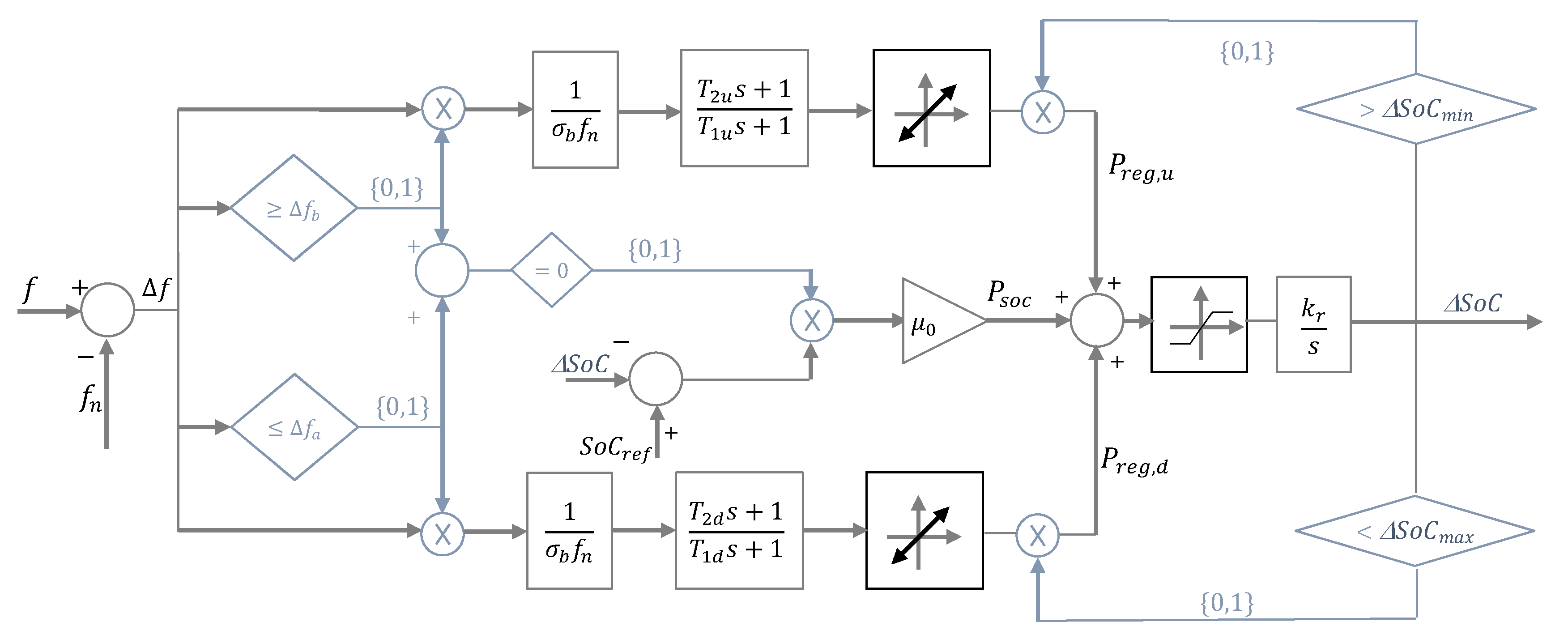
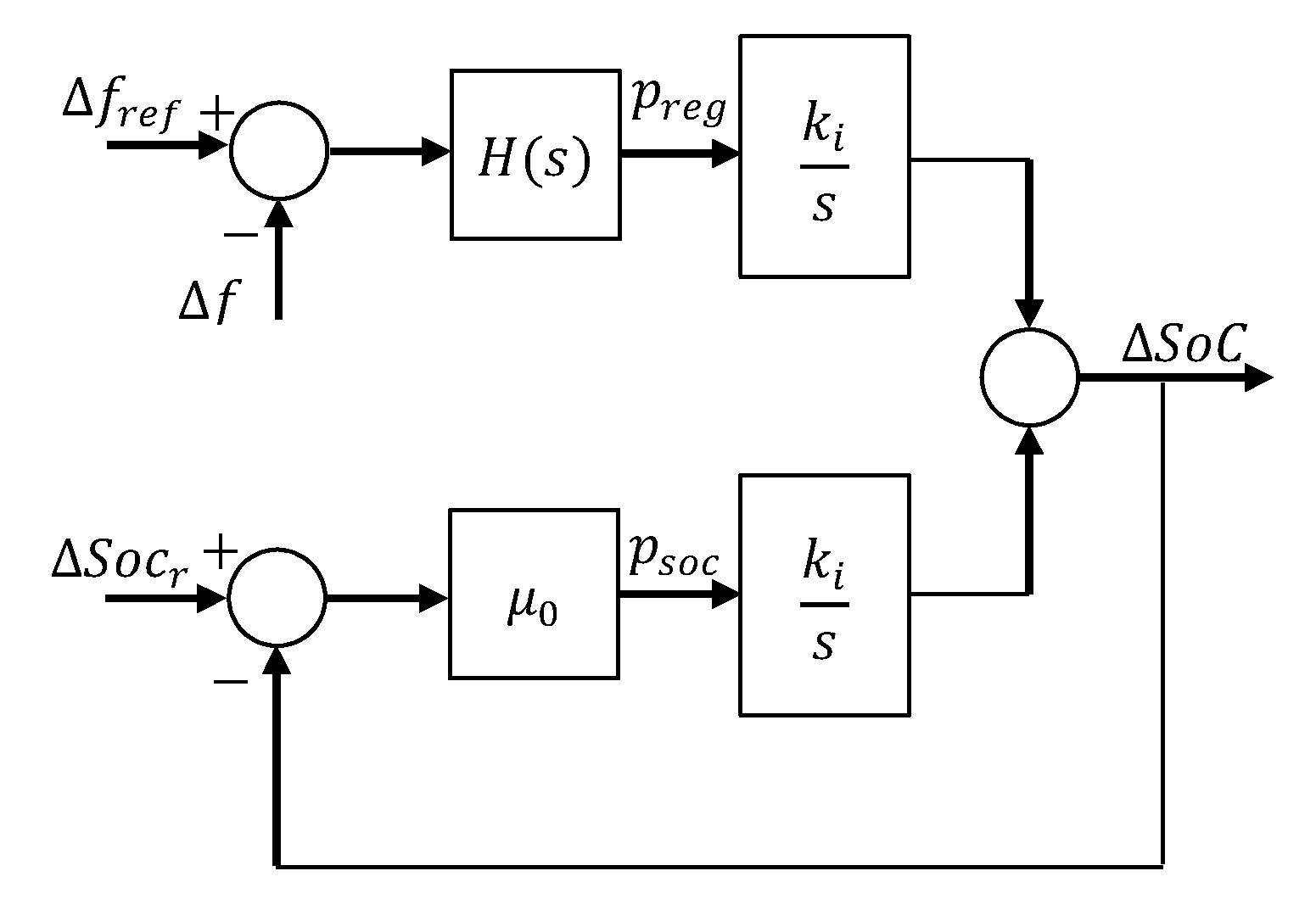
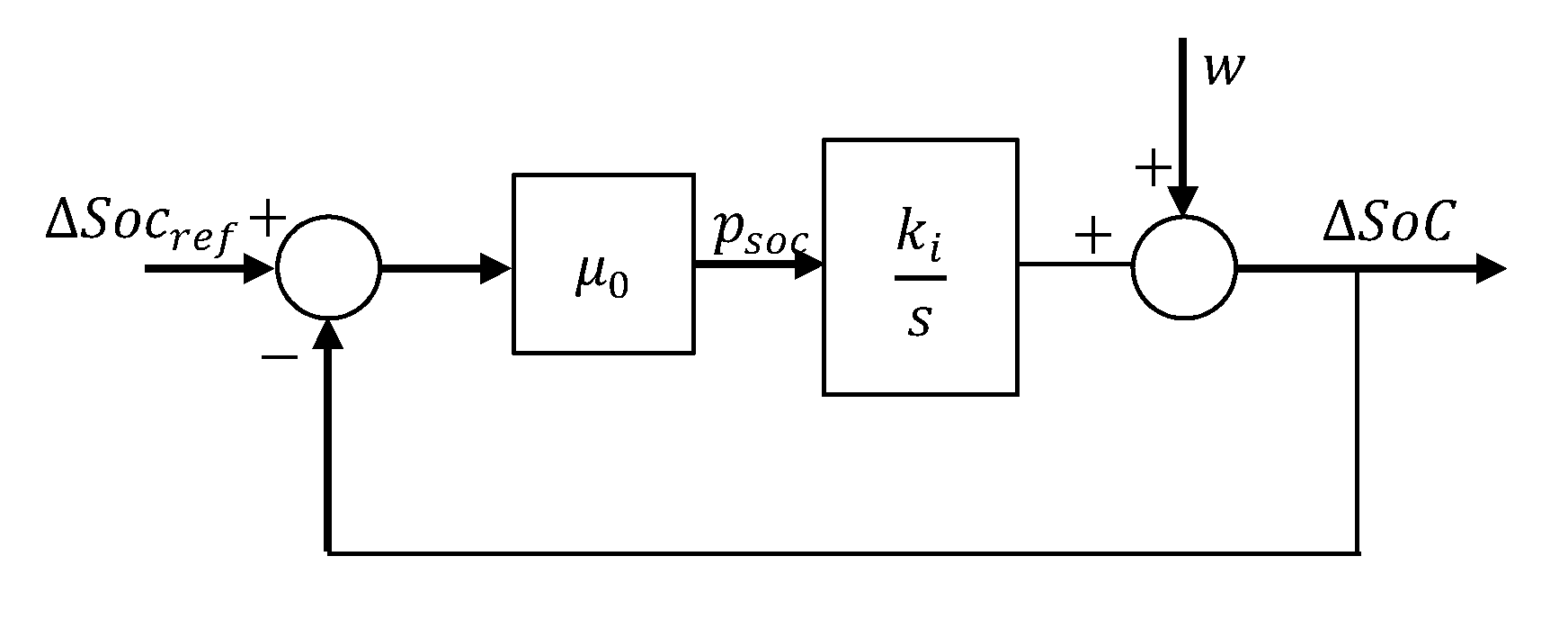
4.4. BESS Control Scheme

The above considerations suggest modifying the control scheme of Figure 3 in that shown in Figure 7. The proposed scheme of Figure 7 allows us to update the regulation power to the SoC level, thereby obtaining a balance between (i) the regulation power needed for the provision of the regulation service and (ii) the need of SoC recovery. This control scheme allows us to simplify the control of the BESS even preserving multiple complex requirements, provided that the correct choice of the gain parameter ${\mu }_0$ is performed. The proposed approach allows us to consider the features of the frequency variations, the requirements imposed by the system operator in the service provided by the BESS, and the range of values within which the SoC must falls. This approach can be used for any battery technology.

In order to derive, that means to design the regulator, it is possible to refer to the control scheme of Figure 6, where the disturbance $w$ has been previously identified as a random walk. The two control blocks above discussed identify two transfer functions:

• $G\left(s\right)$ which relates the output, i.e., $\Delta SoC$, to the disturbance, i.e., $w$.
• $F\left(s\right)$ which relates the output, i.e, $\Delta SoC$, to the input, i.e., $\Delta So{C}_{ref}$.

The two transfer functions can be identified as:

$$G\left(s\right)=\frac{s}{s+{\mu }_0{k}_i}$$

(46)

$$F\left(s\right)=\frac{{\mu }_0{k}_i}{s+{\mu }_0{k}_i}.$$

(47)

$F\left(s\right)$ clearly identifies a low-pass filter, whose cut-off frequency is ${\mu }_0{k}_i$. Thus, the correct evaluation of the proportional gain ${\mu }_0$ must comply with a proper frequency bandwidth, which must be large enough to catch frequencies able to meet the requirements of both frequency regulation and SoC recovery. From one hand, highest cut-off frequency values can keep SoC values closest to its reference value by reducing the effect of the disturbance $w$. On the other hand, in the paper, the disturbance $w$ is modelled to represent the effect of the battery power required for the regulation service. Thus, this reduction must not be too high, that is a proper value of the cut-off frequency must be assigned. In Figure 8, a schematic of the effect of the choice of the cut-off frequency is shown.

The aim of the proposed control method is to define a correction to the BESS output power in the frequency domain which uses high frequency band to provide the desired regulation service and low frequency band to counteract the low frequency drift that takes SoC out of the limits. In order to choose the proper value of the cut-off frequency, the requirements of the power frequency regulation service should be considered. The primary regulation service time interval availability is assumed to be equal to 15 min [20], thus implying that the allowed boundary frequency $f_w$ of the spectral signal $w$ are those corresponding to $\tau =900 \mathrm{s}$, that is:

$$f_w=\frac{1}{900}=1.1 · {10}^{-3} \mathrm{Hz}$$

(48)

which corresponds to the angular frequency, ${\omega }_w$, given by:

$${\omega }_w=2\pi ·1.1 ·{10}^{-3}\cong 7·{10}^{-3}\mathrm{rad}/\mathrm{s}$$

(49)

Eventually, the cut-off frequency of ${\omega }_{cut},$ can be properly chosen as a decade lower, since ${\omega }_w$ allows us to obtain $3\mathrm{dB}$ abatement, so obtaining:

$${\omega }_{cut}=7·{10}^{-4}\mathrm{rad}/\mathrm{s}.$$

(50)

The value of the proportional gain ${\mu }_0$ can finally be given by:

$${\mu }_0=\frac{{\omega }_{cut}}{k_i}$$

(51)

being

$$k_i=\frac{P_n}{ E_n}$$

(52)

5. Numerical Applications

In this section, an analysis is performed on the frequency, the BESS regulation power and the BESS SoC with respect to the stochastic approaches described in Section 3 and Section 4. For the sake of clarity, the results are reported in three sub-sections, related to the (i) analysis of frequency data, (ii) analysis of regulation power, and (iii) analysis of SoC, respectively. The size of the BESS used in the simulation corresponds to a power rating of 98.5 MW and an energy rating of 49.5 MWh [20].

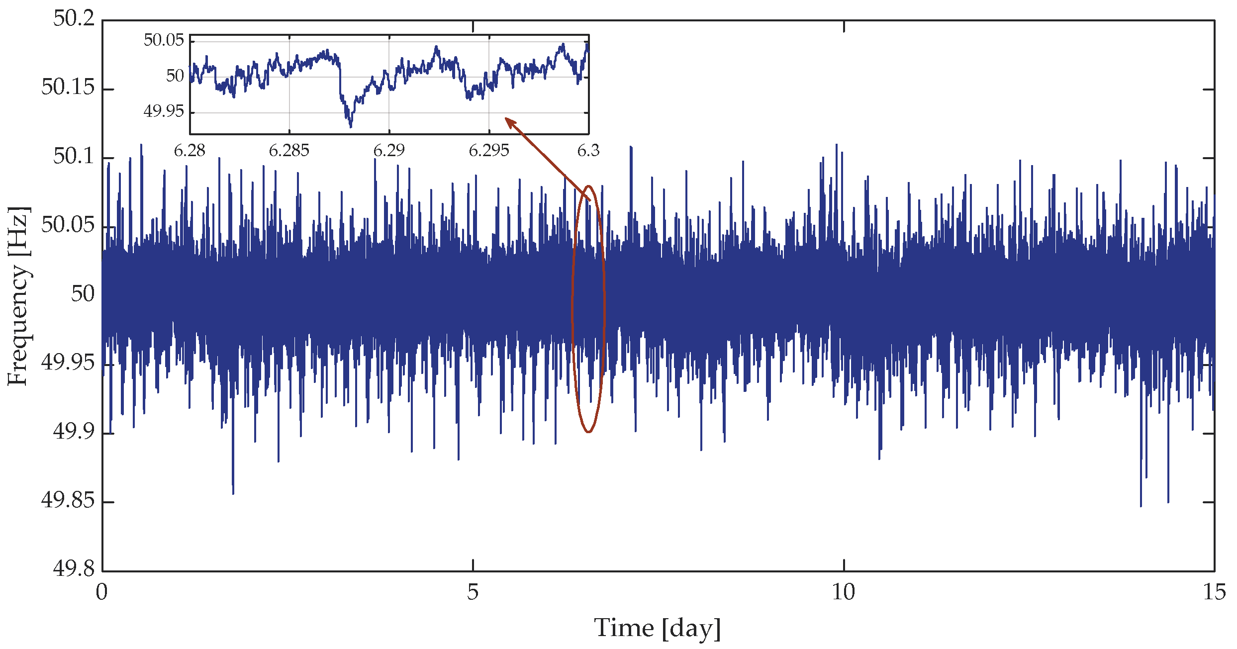
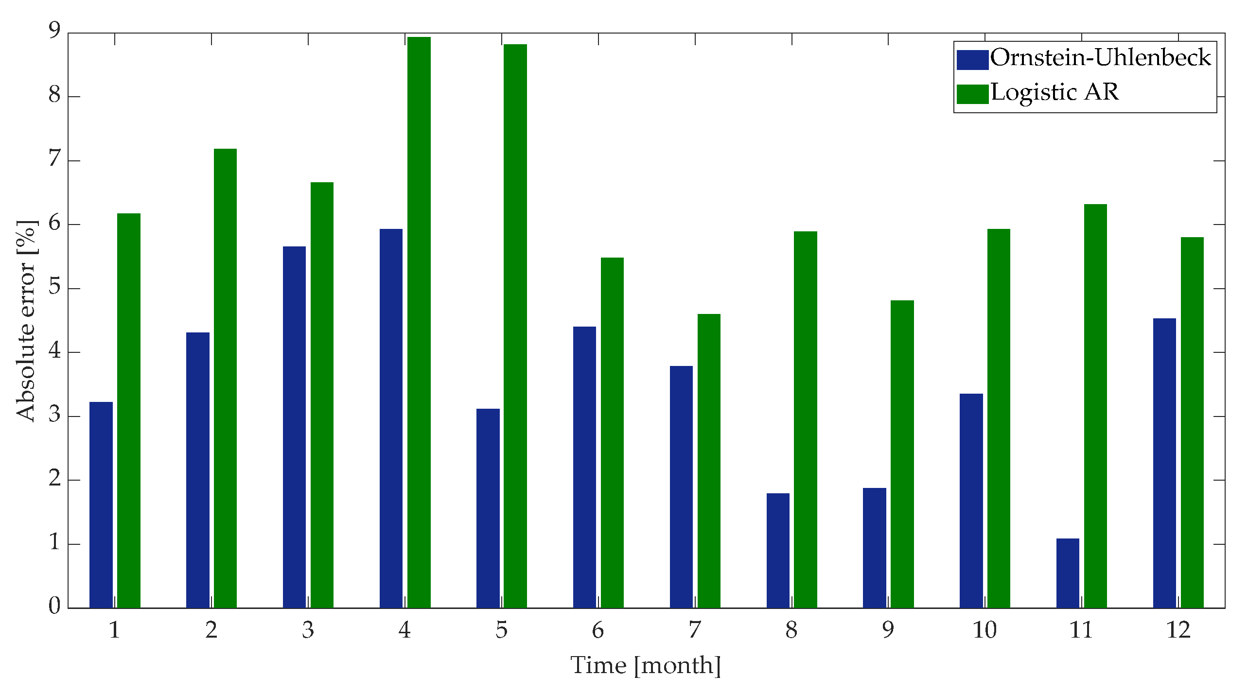
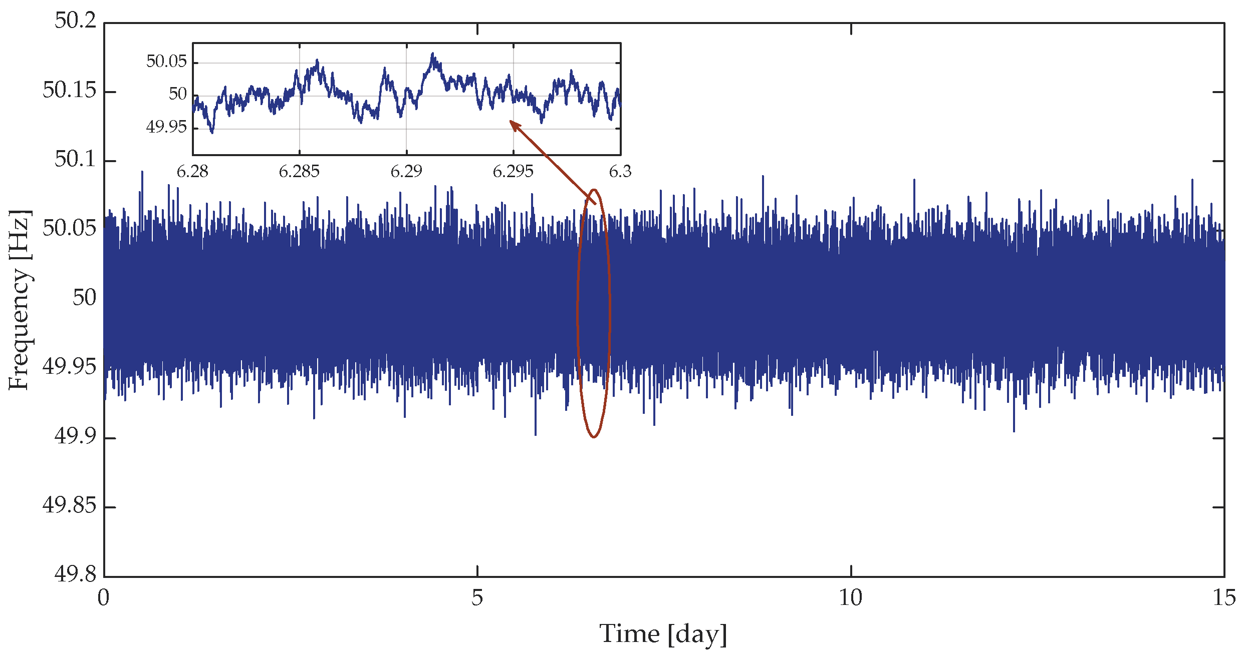
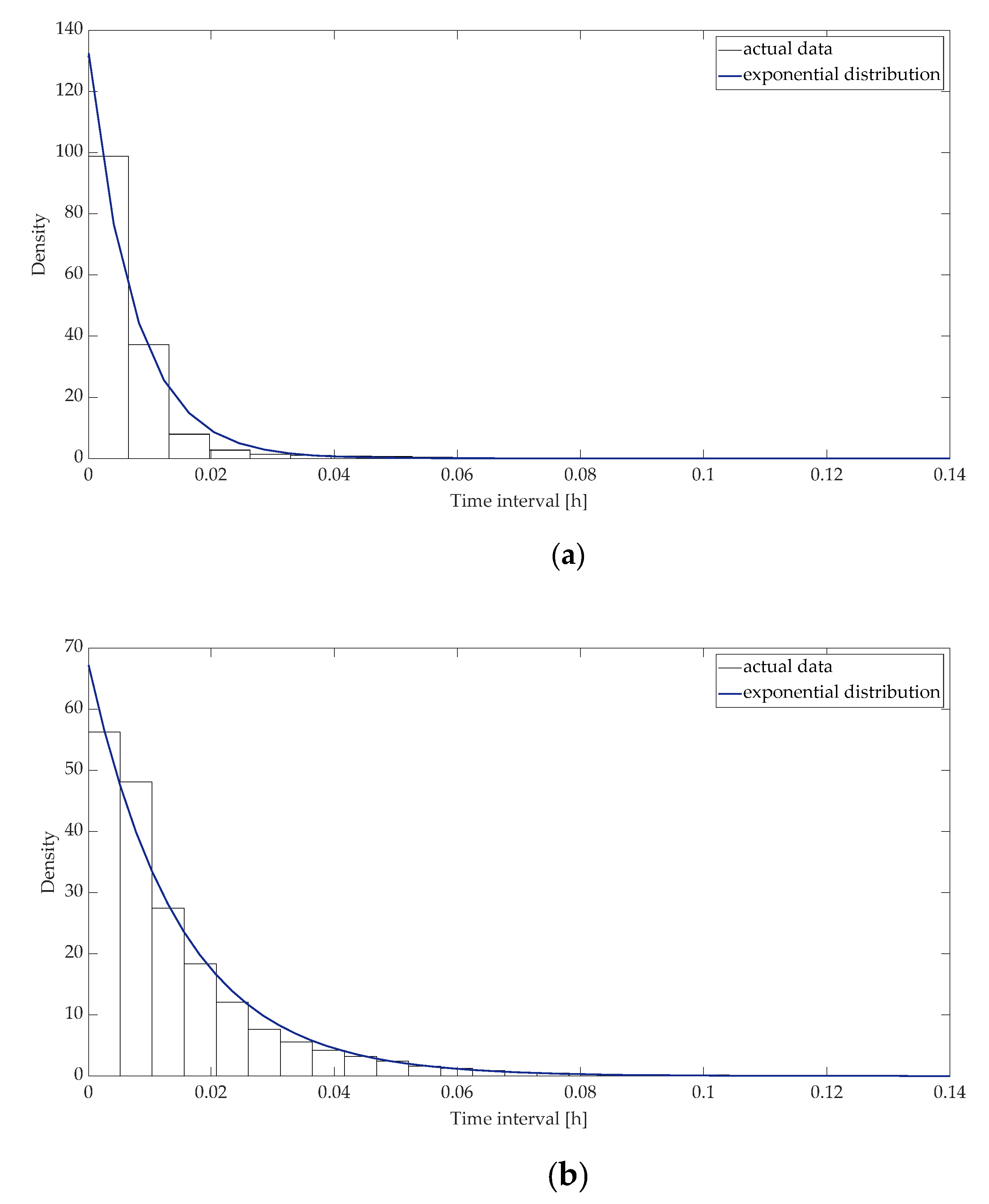
5.1. Analysis of Frequency Data

The analysis of this section refers to the assessment of the stochastic assumptions on the frequency process discussed in Section 3. To test the logistic-autoregressive (logistic AR) and Ornstein–Uhlenbeck processes, actual frequency data were used, made available from the French Transmission operator RTE [28]. More specifically, one-year frequency values from April 2021 to March 2022 were used. In Figure 9 the frequency variation in the period 1–15 April is reported. In the same figure, a zoom of a portion of the April 6th is also reported.

The data under consideration have been used for the stochastic characterization of the frequency with respect to the logistic-AR and Ornstein–Uhlenbeck processes. The effectiveness of the approaches has been analyzed through the method of the moments. At this purpose, the percentage error of the first and second moments evaluated by characterizing the frequency through the logistic-AR and Ornstein–Uhlenbeck processes are reported in Figure 10 and Figure 11. Both the figures refer to the whole set of the available data and the errors are evaluated on a monthly interval basis.

The analysis of Figure 10 and Figure 11 shows that both the processes allow obtaining accurate characterization of the regulation power process. In particular, the Ornstein–Uhlenbeck process generally performs better than the logistic-AR process. Regarding the mean values (Figure 10), both the processes allow us to obtain quite a good estimation of the actual dataset with very low errors. The maximum absolute errors are lower than 1.6·10⁻³% for the Ornstein-Uhlenbeck and 2·10⁻³% for the logistic-AR. Regarding the second moment, the Ornstein-Uhlenbeck always has a lower error than that obtained through the logistic-autoregressive. The maximum absolute error of the Ornstein–Uhlenbeck is less than 6% and that of the logistic-AR is less than 9%. The better performance of the Ornstein–Uhlenbeck process is clearly reported in

Table 1. MAPE Errors.

	Error	Mean [%]	Variance [%]
Process
Monthly
Logistic Autoregressive		7.2 × 10−4	6.2
Ornstein–Uhlenbeck		3.5 × 10−4	3.0
Weekly
Logistic Autoregressive		2.0 × 10−3	8.8
Ornstein–Uhlenbeck		6.8 × 10−4	3.3
Daily
Logistic Autoregressive		6.7 × 10−3	7.9
Ornstein–Uhlenbeck		1.8 × 10−3	5.3

, where the mean absolute percentage error (MAPE) on the first and second moments of both processes are reported for the whole dataset. In the table, the MAPE is reported also with respect to the processes estimated on weakly and daily basis. In all the cases, the MAPE of Ornstein–Uhlenbeck is lower than the logistic-AR process.

The fourth moments (kurtosis) of the two processes have also been compared. In this regard, the better performance of the logistic-AR process demonstrates that it can better reproduce the tails of the distribution of the time series values.

A synthetic profile estimated according to the Ornstein–Uhlenbeck process for seven days is reported in Figure 12. In the same figure, a zoom of a portion of the sixth day is also reported. A qualitative analysis of the comparison between the synthetic (Figure 12) and actual (Figure 9) profiles clearly confirms the accuracy of the Ornstein–Uhlenbeck approach.

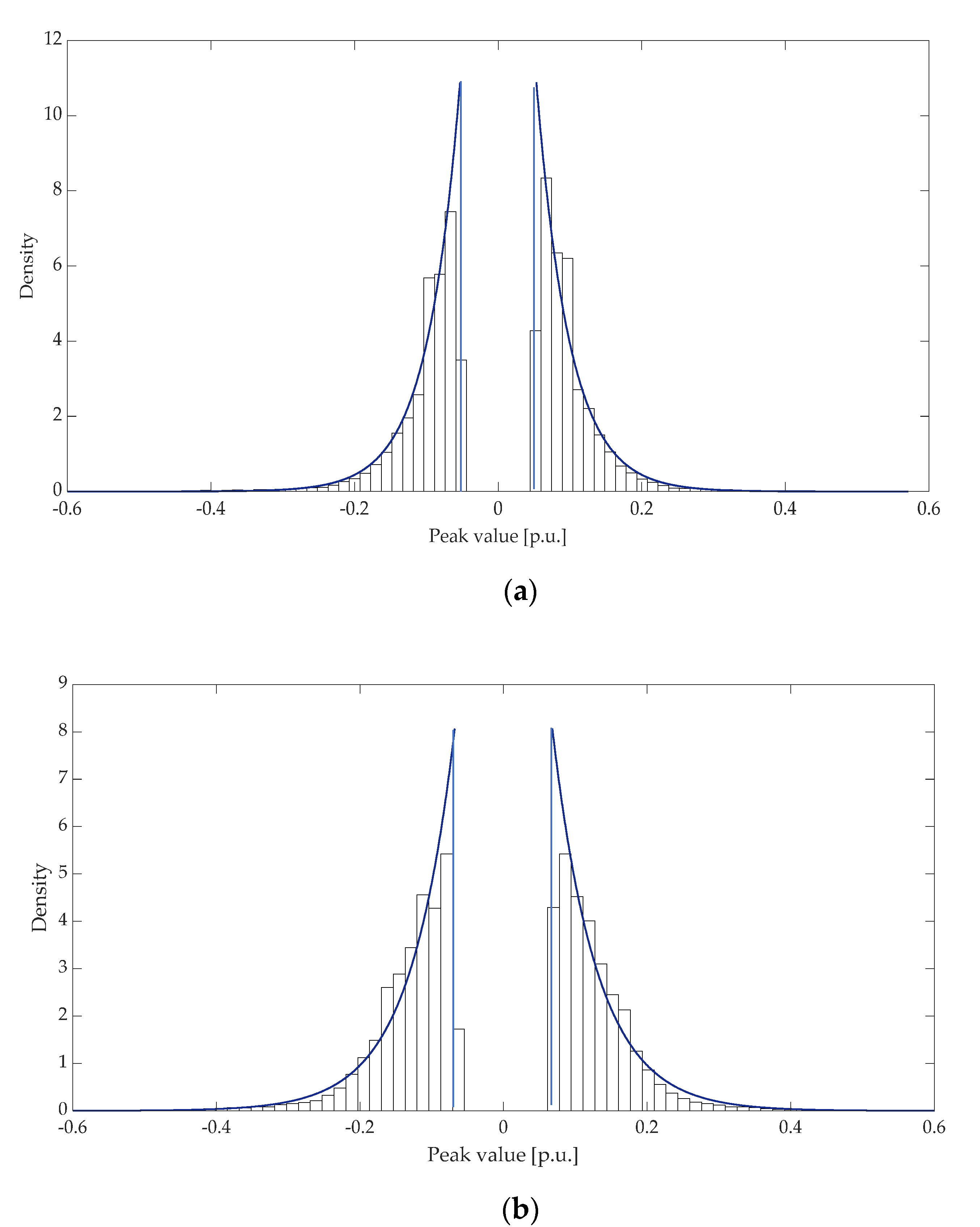
5.2. Analysis of Regulation Power

Based on the control scheme of Figure 3, the regulation power can be evaluated, starting from the real system frequency or that corresponding to the stochastic process modeled according to the Ornstein–Uhlenbeck processes. In what follows, three case studies are reported with respect to three possible scenarios involving the dead-bands:

• Case 1: the dead-band is not considered;
• Case 2: the dead-band is $\pm 10 \text{mHz}$;
• Case 3: the dead-band is $\pm 20 \text{mHz}$.

By neglecting the effect of the SoC recovery control, in Figure 13 an example of the regulation power for the same period of Figure 9 is reported. Case 1, Case 2, and Case 3 are referred to in Figure 13, Figure 14 and Figure 15, respectively. By comparing the zooms of the three cases, the effect of the increasing dead-band range clearly appears.

Based on the method of the moments, an analysis of the regulation power obtained in Case 1 similar to that reported in Section 5.1 (with reference to the frequency) was carried out, showing that it varies according to a Ornstein–Uhlenbeck process.

Regarding the other two cases, where it appeared that the regulation power can be approximated by a Poisson process, a statistical analysis of the amplitudes of the peak values of the regulation power and their time of occurrence was performed. In particular, the amplitude data were given in terms of non-parametric distributions and were compared to the truncated-Laplace distribution. These comparisons are shown in the Figure 16a,b), which correspond to Cases 2 and 3, respectively.

With reference to the data used in this application, the scale parameter of the truncated Laplace distribution is equal to $b_p=0.0459$ in the case of a dead-band equal to $\pm 10 \text{mHz}$ (Case 2), and $b_p=0.0620$ in the case of a dead-band equal to $\pm 20 \text{mHz}$ (Case 3); in both cases the location parameter is ${\mu }_p ≌ 0$.

Regarding the time of occurrence of the regulation power, the analysis of the actual values is reported in Figure 17. In particular, Figure 17a refers to Case 2 and Figure 17b refers to the Case 3. These data are collected in terms of frequency of occurrence whose histograms are reported in the figure together with the fitting exponential distribution which provides an accurate approximation of the real distribution.

In the two cases the mean value ${\mu }_t$ is equal to 0.0074 h (dead-band $\pm 10 \text{mHz}$) and equal to 0.0148 h (dead-band $\pm 20 \text{mHz}$).

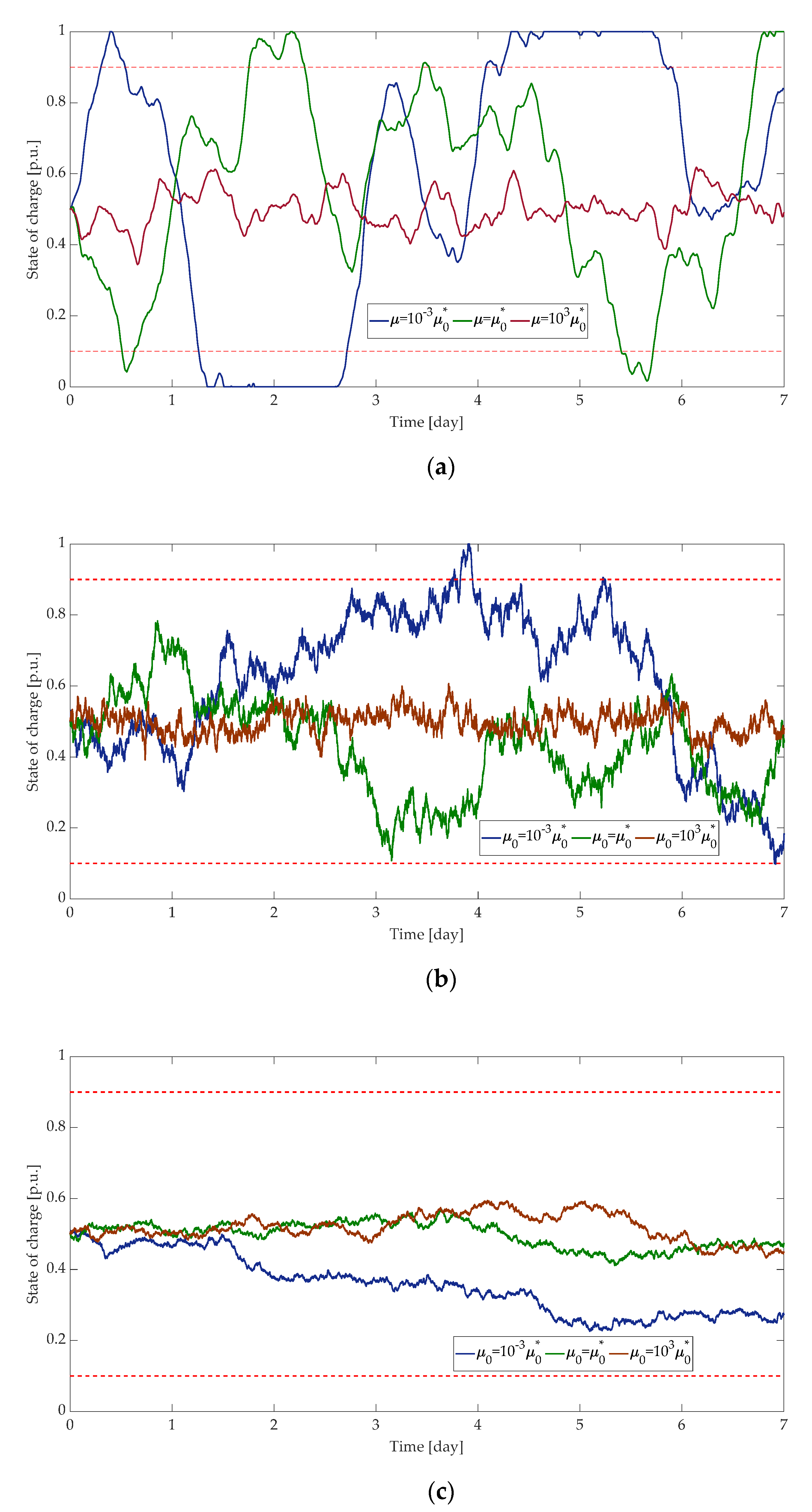
5.3. Analysis of State of Charge

Various simulations have been performed for deriving different SoC profiles corresponding to the three case studies defined in the previous sub-sections, which refer to the different dead-bands. Regarding the gain parameter ${\mu }_0$, the value estimated in Section 4 has been initially considered (${\mu }_0{}^{*}=1.4·{10}^{-3}$). The effect of two further values have also been investigated, which are ${\mu }_0={10}^{-3}{\mu }_0{}^{*}$ and ${\mu }_0={10}^3{\mu }_0{}^{*}$. The SoC profiles obtained for each gain parameter are reported in Figure 18 for each case study: Figure 18a refers to Case 1, Figure 18b refers to Case 2, and Figure 18c refers to Case 3.

The profiles reported in Figure 18a clearly show that, in the absence of a dead-band, the BESS is continuously used for providing power to the grid for frequency regulation. This implies that during the considered time of observation the SoC profile often reaches its maximum and minimum capacity values. Particularly, this happens in the case of ${\mu }_0={\mu }_0{}^{*}$, for which the SoC exceeds, in some cases, the upper (0.9 p.u.) and lower (0.1 p.u.) limits typically adopted for the SoC to preserve the battery lifetime. As expected, the lower value of the gain parameter (${\mu }_0={10}^{-3}{\mu }_0{}^{*}$) implies an even higher use of the battery for frequency regulation thus resulting in a SoC profile that often exceeds the admissible limits. On the contrary, a greater value of the gain parameter (${\mu }_0={10}^3{\mu }_0{}^{*}$) implies less participation of the battery to the frequency regulation service, thus resulting in a SoC profile that is contained within a narrow range around the reference value of 0.5 p.u. This consideration is fundamental since it demonstrates that a proper choice of ${\mu }_0$ is required to optimally design the control action of the BESS which guarantees the lifetime preservation.

The considerations made for Case 1 also apply to the case of Figure 18b which refers to a dead-band of ±10 mHz (Case 2). However, the presence of the dead-band implies a lower participation of the BESS to the frequency regulation, thus implying that the SOC profile has lower variations than that of the previous case and the SOC limits are rarely reached. This behavior is stressed in the case of dead-band at ±20 mHz (Case 3) for which the SoC always ranges in an interval very close to the reference value of 0.5 p.u. This value of the dead-band implies oversizing of the BESS.

In summary, the plots of Figure 18 show that, when the value of the parameter is optimally chosen, the BESS control is optimized, since it is controlled by maintaining the SoC within admissible ranges, thus optimizing the provision of the regulation service. When the parameter is lower than the optimal value, the SoC profile exceeds the admissible range; differently, when the parameter is greater than the optimal value, the SoC varies very slowly. As expected, the figures also show that the effect of the parameter value depends on the dead-band width.

By comparing the SoC profiles of Figure 18, it is clear that in case of Figure 18a the profile is smoother than that obtained in Figure 18b,c. This is obviously due to the nature of the stochastic process of the regulation power, which is an Ornstein–Uhlenbeck process in case of Figure 18a (absence of the dead-band), and is a compound Poisson process in case of Figure 18b,c (presence of the dead-band). The presence of jumps in the compound Poisson process, indeed, implies the presence of spikes in the profiles of SoC.

6. Conclusions

In this paper, a new stochastic approach has been applied to the study of the primary frequency regulation service provided by battery energy storage systems. The use of storage devices for frequency regulation in modern power systems is influenced by complexities due to the need to match the requirements imposed by the transmission system operators for the provision of the service, and the containment of the battery lifetime degradation, imposed by the economic issues. For this purpose, proper control strategies are requested to be designed which can be used despite the uncertainties typically affecting the frequency regulation service. In this application, a stochastic approach is proposed to provide accurate models for the time profiles of frequency, regulation power, and state of charge. In particular, the use of the Ornstein–Uhlenbeck stochastic process is studied for the frequency profile. Regarding the regulation power, it has been proven that it can still be modeled according to the Ornstein–Uhlenbeck process or the compound Poisson process, depending on the service performance requested of the storage device (more specifically, depending on the presence or absence of the dead-band). It has been demonstrated that, in both cases, the state of charge can be modeled according to an Ornstein–Uhlenbeck process driven by an Ornstein–Uhlenbeck process. The accuracy of this approach has been investigated in this paper together with the definition of a gain parameter, which can be set appropriately to optimize the control of the battery for the balance between availability of regulation service and battery lifetime degradation. In the numerical application it has been found that this problem can be studied as a hitting problem, for which more research efforts are needed in future works. The proposed approach also makes the primary frequency regulation service provided by battery energy storage systems prone to the use of stochastic control methods which inherently account for the existence of uncertainties in the evolution of the system frequency.

References

1. Brivio, C.; Mandelli, S.; Merlo, M. Battery energy storage system for primary control reserve and energy arbitrage. Sustain. Energy Grids Netw. 2016, 6, 152–165. [Google Scholar] [CrossRef]
2. Guerra, K.; Haro, P.; Gutiérrez, R.E.; Gómez-Barea, A. Facing the high share of variable renewable energy in the power system: Flexibility and stability requirements. Appl. Energy 2022, 310, 118561. [Google Scholar] [CrossRef]
3. Carlini, E.M.; Del Pizzo, F.; Giannuzzi, G.M.; Lauria, D.; Mottola, F.; Pisani, C. Online analysis and prediction of the inertia in power systems with renewable power generation based on a minimum variance harmonic finite impulse response filter. Int. J. Electr. Power Energy Syst. 2021, 131, 107042. [Google Scholar] [CrossRef]
4. IRENA. Battery Storage for Renewables: Market Status and Technology Outlook. 2015. Available online: https://www.irena.org/publications/2015/Jan/Battery-Storage-for-Renewables-Market-Status-and-Technology-Outlook (accessed on 4 July 2022).
5. Thien, T.; Axelsen, H.; Merten, M.; Axelsen, H.; Merten, M.; Zurmùhlen, S.; Münderlein, J.; Leuthold, M.; Sauer, D.U. Planning of grid-scale battery energy storage systems: Lessons learned from a 5 MW hybrid battery storage project in Germany. In Proceedings of the Battcon International Stationary Battery Conference, Orlando, FL, USA, 12–14 May 2015. [Google Scholar]
6. Fu, H.; Tong, X.; Pan, Z.; Liu, F.; Wang, F.; Zhang, W. Research on BESS Participating in Power System Primary Frequency Regulation Control Strategy Considering State-of-Charge Recovery. In Proceedings of the 5th International Conference on Energy, Electrical and Power Engineering, Chongqing, China, 22–24 April 2022. [Google Scholar]
7. Oudalov, A.; Chartouni, D.; Ohler, C. Optimizing a Battery Energy Storage System for Primary Frequency Control. IEEE Trans. Power Syst. 2007, 22, 1259–1266. [Google Scholar] [CrossRef]
8. Stroe, D.; Knap, V.; Swierczynski, M.; Stroe, A.; Teodorescu, R. Operation of a Grid-Connected Lithium-Ion Battery Energy Storage System for Primary Frequency Regulation: A Battery Lifetime Perspective. IEEE Trans. Ind. Appl. 2017, 53, 430–438. [Google Scholar] [CrossRef]
9. Khalid, M.; Savkin, A.V. An optimal operation of wind energy storage system for frequency control based on model predictive control. Renew. Energy 2012, 48, 127–132. [Google Scholar] [CrossRef]
10. Andrenacci, N.; Chiodo, E.; Lauria, D.; Mottola, F. Life Cycle Estimation of Battery Energy Storage Systems for Primary Frequency Regulation. Energies 2018, 11, 3320. [Google Scholar] [CrossRef]
11. Wu, F.; Sioshansi, R. A stochastic operational model for controlling electric vehicle charging to provide frequency regulation. Transp. Res. Part D Transp. Environ. 2019, 67, 475–490. [Google Scholar] [CrossRef]
12. Scarabaggio, P.; Carli, R.; Cavone, G.; Dotoli, M. Smart Control Strategies for Primary Frequency Regulation through Electric Vehicles: A Battery Degradation Perspective. Energies 2020, 13, 4586. [Google Scholar] [CrossRef]
13. Meng, G.; Lu, Y.; Liu, H.; Ye, Y.; Sun, Y.; Tan, W. Adaptive Droop Coefficient and SOC Equalization-Based Primary Frequency Modulation Control Strategy of Energy Storage. Electronics 2021, 10, 2645. [Google Scholar] [CrossRef]
14. Tan, Z.; Li, X.; He, L.; Li, Y.; Huang, J. Primary frequency control with BESS considering adaptive SoC recovery. Int. J. Electr. Power Energy Syst. 2020, 117, 105588. [Google Scholar] [CrossRef]
15. Shim, J.W.; Verbič, G.; Kim, H.; Hur, K. On Droop Control of Energy-Constrained Battery Energy Storage Systems for Grid Frequency Regulation. IEEE Access 2019, 7, 166353–166364. [Google Scholar] [CrossRef]
16. Dang, J.; Seuss, J.; Suneja, L.; Harley, R.G. SOC feedback control for wind and ESS hybrid power system frequency regulation. In Proceedings of the IEEE Power Electronics and Machines in Wind Applications Conference, Denver, CO, USA, 16–18 July 2012. [Google Scholar]
17. Marconato, R. Electric Power Systems Vol. 2: Steady-State Behaviour Controls, Short Circuits and Protection Systems, 2nd ed.; CEI: Milan, Italy, 2004. [Google Scholar]
18. Vorobev, P.; Greenwood, D.M.; Bell, J.H.; Bialek, J.W.; Taylor, P.C.; Turitsyn, K. Deadbands, Droop, and Inertia Impact on Power System Frequency Distribution. IEEE Trans. Power Syst. 2019, 34, 3098–3108. [Google Scholar] [CrossRef]
19. Quint, R.; Ramasubramanian, D. Impacts of droop and deadband on generator performance and frequency control. In Proceedings of the IEEE Power and Energy Society General Meeting, Chicago, IL, USA, 16–20 July 2017. [Google Scholar]
20. Knap, V.; Chaudhary, S.K.; Stroe, D.I.; Swierczynski, M.; Craciun, B.I.; Teodorescu, R. Sizing of an Energy Storage System for Grid Inertial Response and Primary Frequency Reserve. IEEE Trans. Power Syst. 2016, 31, 3447–3456. [Google Scholar] [CrossRef]
21. del Giudice, D.; Brambilla, A.; Grillo, S.; Bizzarri, F. Effects of inertia, load damping and dead-bands on frequency histograms and frequency control of power systems. Int. J. Electr. Power Energy Syst. 2021, 129, 106842. [Google Scholar] [CrossRef]
22. Brockwell, P.J.; Davis, R.A. Introduction to Time Series and Forecasting, 2nd ed.; Springer: New York, NY, USA, 2002. [Google Scholar]
23. Kallas, M.; Honeine, P.; Richard, C.; Francis, C.; Amoud, H. Prediction of time series using Yule-Walker equations with kernels. In Proceedings of the IEEE International Conference on Acoustics, Speech and Signal Processing (ICASSP), Kyoto, Japan, 25–30 March 2012. [Google Scholar]
24. Hassanzadeh, M.; Evrenosoğlu, C.Y.; Mili, L. A Short-term nodal voltage phasor forecasting method using temporal and spatial correlation. IEEE Trans. Power Syst. 2016, 31, 3881–3890. [Google Scholar] [CrossRef]
25. Wong, W.K.; Bian, G. Estimating parameters in autoregressive models with asymmetric innovations. Stat. Probab. Lett. 2005, 71, 61–70. [Google Scholar] [CrossRef]
26. Holý, V.; Tomanová, P. Estimation of Ornstein-Uhlenbeck Process Using Ultra-High-Frequency Data with Application to Intraday Pairs Trading Strategy. arXiv 2019, arXiv:1811.09312v2. [Google Scholar]
27. Smith, P.L. From Poisson shot noise to the integrated Ornstein–Uhlenbeck process: Neurally principled models of information accumulation in decision-making and response time. J. Math. Psychol. 2010, 54, 266–283. [Google Scholar] [CrossRef]
28. RTE. Network Frequency. Available online: https://www.services-rte.com/en/view-data-published-by-rte.html (accessed on 4 July 2022).
Figure 1. Block diagram for analyzing the frequency transients.
Energies 15 06508 g001
Figure 2. The action of the BESS for the primary frequency regulation service.
Energies 15 06508 g002
Figure 3. Block diagram of the BESS control strategy for primary frequency regulation.
Energies 15 06508 g003
Figure 4. Block diagram of the battery control strategy.
Energies 15 06508 g004
Figure 5. Action of the BESS for the primary frequency regulation service in the absence of the dead-band.
Energies 15 06508 g005
Figure 6. Block diagram of the SoC control scheme.
Energies 15 06508 g006
Figure 7. SoC control scheme.
Energies 15 06508 g007
Figure 8. Cut-off frequency choice criterion.
Energies 15 06508 g008
Figure 9. Actual frequency data from 1–15 April.
Energies 15 06508 g009
Figure 10. Errors of the mean evaluated with characterization by logistic–AR and Ornstein–Uhlenbeck processes.
Energies 15 06508 g010
Figure 11. Errors of the second moments evaluated with characterization by logistic–AR and Ornstein–Uhlenbeck processes.
Energies 15 06508 g011
Figure 12. Frequency data estimated according to the Ornstein–Uhlenbeck process.
Energies 15 06508 g012
Figure 13. Regulation power in Case 1.
Energies 15 06508 g013
Figure 14. Regulation power in Case 2.
Energies 15 06508 g014
Figure 15. Regulation power in Case 3.
Energies 15 06508 g015
Figure 16. Approximation of the power peak values of the regulation power to a Laplace pdf in Case 2 (a) and Case 3 (b).
Energies 15 06508 g016
Figure 17. Approximation of the time occurrence of regulation power to an exponential pdf in Case 2 (a) and Case 3 (b).
Energies 15 06508 g017
Figure 18. Examples of synthetic SoC profiles over a week in Case 1 (a), Case 2 (b), and Case 3 (c).
Energies 15 06508 g018