Abstract
The design of an adsorption solar air conditioning system is investigated by using a model with an activated carbon–methanol working pair. This system is analysed with the solar insolation levels and ambient temperatures of Singapore. The proposed design mainly consists of two tubular reactor heat exchangers (TRHEXs) operating out of phase and driven by heat from an evacuated tube solar collector (ETSC). The pair of TRHEXs act as a thermal compressor and contain about 2.275 kg of activated carbon per reactor. The evacuated tube solar collector (ETSC) has better performance and is more cost effective than the flat plate solar collector (FPSC), even though it has a higher cost per unit. On the hottest day of the year, the proposed adsorption system has a maximum cooling power of 2.6 kW and a COP of 0.43 at a maximum driving temperature of 139 °C with a 9.8 m2 ETSC area. The system has a total estimated cost of EUR 10,550 corresponding to about SGD 14,800 with a 7-year payback time. At similar cooling capacities, the adsorption air conditioning system is expected to be more cost effective than the conventional system beyond an expected period of 7 years, with an expected lifetime of 15 to 20 years.
1. Background and Introduction
Climate change is a growing global issue. One of the largest contributors is the release of greenhouse gases due to increasing electricity demand. As much as MW of solar power from the sun is intercepted by the earth, far in excess of the present power consumption. There is also huge potential to better utilise waste heat sources emitted from existing systems and processes. By utilising this huge amount of renewable and waste heat energy, the current and future energy requirements of the world can easily be fulfilled. Air conditioning systems have been increasing in usage due to rising global temperatures leading to increased electricity consumption. There is hence a need to reduce electricity usage for these systems. Adsorption air conditioning systems driven by solar energy are attractive, since the peak cooling demand coincides with peak solar insolation during the day.
By 2050, global energy usage for cooling is expected to triple, while in hotter countries such as China, India, and Indonesia, it is expected to increase five-fold [1]. This would lead to higher global energy demands for cooling than heating by the end of the century. In 2018, Singapore consumed 50 TWh of electricity and 60 PJ of natural gas [2]. The non-residential building sector took up 31% of total electricity consumption by end-use, with 60% of that used solely for air conditioning [3]. With climate change causing higher ambient temperatures, electricity consumption for air conditioning would likely increase. With an average annual solar irradiance of 1600 kWh/m2, solar energy is the most viable renewable energy source in Singapore. However, electricity generation by solar photovoltaic only accounted for 0.8% of total electricity generation in 2018 [2]. As a developed country with access to the newest advances in technology, Singapore has the capacity to adopt better systems to generate electricity through solar energy. The average price of electricity in Singapore in 2019 was about 24.22 cents/kWh [4].
A conventional vapour compression air conditioning system with a rated cooling capacity of 2.5 kW, such as the Smart ENVi model [5], would lead to a usage cost of about SGD 6, including various taxes for 10 h operation in Singapore. A year of such daily usage results in an electricity cost of SGD 2135. With an average maintenance cost of SGD 50 every three months, the total annual running cost for a conventional air conditioning unit is about SGD 2335. This estimation is reasonable [6]. A typical air conditioning unit with a 2.5 kW cooling capacity costs about SGD 1200. With such usage and maintenance, the average lifespan of an air conditioning unit in Singapore is about 7 years.
Singapore is a hot and humid country, with ambient temperatures often exceeding 30 °C during the day and an average humidity level of 80%. Due to its year-round tropical climate, air conditioning usage is especially high in Singapore, which has 0 heating degree days (HDD) and 6367 cooling degree days (CDD) per annum [7]. However, an overwhelming majority of air conditioning systems are vapour compression systems mainly reliant on grid electricity. Adsorption systems have low economic viability at present in comparison to conventional vapour compression technologies that are well established in the market. While environmentally friendly and requiring low maintenance, adsorption systems are currently bulky, heavy, and have a high capital cost. The development of an efficient and compact adsorption air conditioning system can potentially complement conventional air conditioning systems, reducing the consumption of non-renewable power sources. Furthermore, less developed areas which lack an electrical grid for conventional air conditioning will also be able to use such technology to improve their quality of life, with little to no detriment to the environment. This great potential for utilising solar energy makes such systems attractive for research. Several buildings in Germany and France have already been using small-scale adsorption cooling installations for refrigeration and air conditioning [8]. The market share of solar sorption cooling technology is steadily growing in Europe, as well as worldwide [9].
The objective of this work is to incorporate a model of a solar collector into a modified existing adsorption model and to create several tools to weigh the benefits of different designs based on cost, specific cooling power (SCP), and coefficient of performance (COP) of the system. Furthermore, a suitable adsorption air conditioning system is proposed for use in Singapore to reduce electricity consumption due to cooling.
2. Adsorption Air Conditioning Model
The full layout of the proposed system is illustrated in Figure 1. The green, blue, and red loops represent the refrigerant, cooling, and heating loops, respectively. The condenser and cooler are under air flow at ambient temperature, which determines their operating temperatures. The thermal energy is transferred from the solar collector to the beds through the heating loop during heating. In the refrigerant loop, as the refrigerant evaporates and absorbs heat in the evaporator, heat is taken away from the cold space to produce the cooling effect. The solenoid valve (SV1) between the two beds allows for refrigerant mass transfer (a process that improves both COP and cooling power). The mass transfer between the two beds takes place at the end of each half cycle.
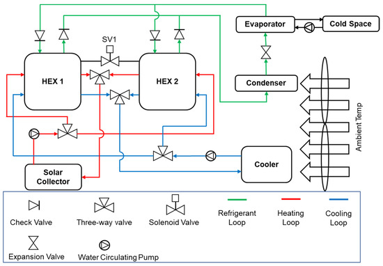
Figure 1.
Layout of a two-bed adsorption air conditioning system [10].
The adsorption air conditioning model was created in MATLAB@ R2020b and is a finite difference model. The model operates on a two-bed adsorption system with heat and mass recovery to enhance the system performance. The model from previous research work [10] was built on and expanded to include different solar collector types, and hourly and monthly Singapore weather data. The weather data were obtained from METEONORM@7.V7.32 and include hourly and monthly solar insolation levels and ambient temperatures averaged from 1991 to 2010. The model uses compacted SRD1352/3 activated carbon as the adsorbent and methanol as the refrigerant, while the HTF used is water. Furthermore, the reactor beds are the miniaturised tube type of heat exchanger (MT-THEX), instead of the micro-channel plate type of heat exchanger (MCP-HEX), as in previous investigations [11,12,13]. The choice of activated carbon as the adsorbent is guided by its high surface area leading to high sorption capacity, by its low cost (less than USD 1 per kg) and its worldwide availability. The choice of methanol as the refrigerant is due to its high latent heat of vaporization per unit volume (typically 872 MJ/m3) and low global warming potential.
2.1. Thermal Compressor
A CAD drawing of the MT-HEX was made using SOLIDWORKS@ in Figure 2, with the dimensions in mm. The shell is made of stainless steel (SS 316) with a length of 315 mm, an outer diameter (OD) of 152.4 mm, and a thickness of 1.63 mm (standard pipe size). The two lids on both sides of the tube have an OD of 152.4 mm and a thickness of 2 mm. There are 800 micro-tubes with an OD of 1.2 mm, an inner diameter (ID) of 0.8 mm, and a length of 315 mm within the outer tube. The micro-tubes also extend through the tube end plates for water manifold connection. The HTF is pumped through the micro-tubes to heat/cool the carbon during desorption/adsorption. The space within the shell between the micro-tubes is filled with compacted SRD1352/3 activated carbon from Chemviron Carbon Ltd.
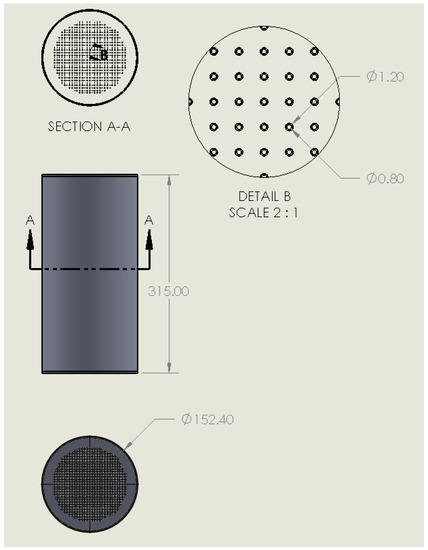
Figure 2.
CAD drawing of tube heat exchanger (dimensions in mm) [10].
For simplicity, the compacted activated carbon is assumed to form a cylinder-like shape around each micro-tube, as illustrated in Figure 3. The estimations of the carbon thickness around each micro-tube , as well as the overall heat transfer coefficient (UA) values, are based on this assumption. Further assumptions are the unidirectional heat flow (radially), longitudinally uniform temperature of the activated carbon bed, and fully developed flow of HTF inside the micro-tube.
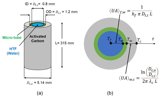
Figure 3.
Micro-tube with activated carbon (a) configuration; (b) model.
The heat transfer between the HTF and the steel wall is calculated using the log mean temperature difference method:
where is the log mean temperature difference between the HTF and the steel wall.
The governing equations of the model consist of the energy balance of the key constituents, namely, the stainless-steel wall, the HTF, and the activated carbon bed with refrigerant uptake:
where are the mass (in kg) of steel wall, HTF, and carbon in the HEX tube, respectively; are the temperature (in K) of the steel wall, HTF, and carbon, respectively; are the specific heat capacity at constant pressure (in Jkg−1 K−1) of the steel wall, HTF, carbon, and methanol, respectively; is the HTF mass flow rate (in kg s−1) through the MT-HEX; and is the concentration of adsorbed methanol in activated carbon (in kg kg−1).
Equations (5) and (6) are used to calculate the carbon and HTF UA values, respectively:
where and are the OD and ID of the carbon (in m) around each micro-tube, L is the length (in m) and λc is the effective thermal conductivity of the activated carbon bed (in W m−1 K−1).
where is the ID of the micro-tube (in m), L is the length (in m) and hf is the effective convective heat transfer coefficient between the HTF and the micro-tube wall (in W m−2 K−1).
The Nusselt number (Equation (7)) is used to calculate the HTF convection heat transfer coefficient (Equation (8)):
where Nu is Nusselt number, is the ID of the micro-tube (in m) and is the thermal conductivity of HTF (in W m−1 K−1).
The flow velocity in each micro-tube was calculated under the assumption of the equal distribution of HTF volumetric flow rate in the micro-tubes:
where is the HTF flow rate through a micro-tube (in m s−1), is the HTF volumetric flow rate through the tube HEX (in m3 s−1), and is the number of micro-tubes.
The Reynolds number was calculated with the following expression:
where is the density of the HTF (in kg m−3), is the HTF velocity in each micro-tube (in m s−1), is the inner diameter of the micro-tube (in m), and is the dynamic viscosity of the HTF (in kg m−1 s−1).
The total flow rate, number of micro-tubes and area of micro-tubes is such that the flow will always be laminar. In the literature [14,15], where the HTF flow is under a uniform and constant surface heat flux, the Nusselt number (Nu) = 4.36, and where the HTF flow is under a uniform surface temperature, Nu = 3.66. In the adsorption system, the heat transfer regime lies somewhere between uniform surface temperature and uniform surface heat flux and, therefore, a Nusselt number of 4 was assumed in the model (corresponding to the average of the two values).
It is often assumed that the refrigerant absorbed by any sorbent is in the form of saturated liquid at the sorbent temperature itself. The specific heat capacity of methanol liquid is, therefore, assumed to be a function of carbon temperature (Tc) and is given by the following linear best fit expression using numerical data from the literature [16]:
where is in J kg−1 K−1 and the carbon temperature Tc is in K.
is given by the following expression obtained from Turner [17] from experimental data:
where is in J kg−1 K−1 and the carbon temperature Tc is in K.
is the specific enthalpy of sorption of methanol (in J kg−1) and is given by the following equation:
where is the slope of the saturated methanol line on the Clapeyron diagram (see Equation (14)), is the carbon temperature (in K), is the saturation temperature of methanol (in K) (which during the cycle will be the condensing temperature, Tcon, during desorption and the evaporating temperature, Tevap, during adsorption) and R is the gas constant of methanol (in J kg−1 K−1) at the carbon bed saturated pressure (Pb,sat) corresponding to carbon temperature (Tc).
where P is pressure in the bar, T is in K, K and .
R is given by the following linear best fitted expression using numerical data from the literature [16]:
The HTF thermal mass is lumped with the wall thermal mass as an approximation to simplify the governing equations, such that Equations (2) and (3) become Equations (16) and (17), respectively:
The model is based on an ideal cycle which assumes that adsorption and desorption are isobaric, which allows Equations (16) and (17) to be integrated through time by substituting for in Equation (4) with Equation (18):
The concentration of adsorbed methanol in the carbon is calculated using a modified Dubinin–Astakhov (D–A) equation, as presented by Critoph [18,19]:
where is the maximum refrigerant concentration (in kg kg−1), and K and n are D–A equation constants.
The partial derivatives of Equation (19) can be calculated analytically as:
The model operates as a two-bed adsorption system with heat and mass recovery between the heating/cooling phases. Mass recovery is carried out by connecting the two adsorbent beds through the methanol loop until their pressures have equalised. This is achieved by taking small concentration change steps in which the high-pressure (HP) bed drops in uptake and the low-pressure (LP) bed increases in uptake by an amount ∆x resulting in the following temperature difference between the two beds (HP and LP):
where Tc,HP and Tc,LP are the high-pressure and low-pressure carbon beds, respectively (in K).
The saturation temperature, and thereby the bed pressure, after the uptake step of ∆x is calculated using Equation (19). This operation is repeated until both bed pressures are equal.
The effective heat input per cycle (in J) is calculated after the steel wall, HTF, and carbon temperature profiles have been established. Table 1 shows the MT-HEX reactor model parameters.

Table 1.
MT-HEX reactor model parameters.
2.2. Evaporator
The specific cooling energy (J kg−1 carbon) is characterized by the latent heat of vaporisation of the methanol liquid collected during the condensation phase:
where is the amount of methanol collected during condensation (in kg kg−1 carbon), is the specific enthalpy of superheated methanol vapour at the evaporating temperature (in J kg−1), and is the specific enthalpy of saturated methanol liquid at the condensing temperature (in J kg−1).
is the amount of cooling energy per cycle (in J) and is given by:
where mc is the mass of carbon (in kg).
The specific cooling power (SCP) is defined by the following expression:
where is the cycle time (in s).
2.3. System Coefficient of Performance (COP)
The coefficient of performance (COP) is calculated from the following equation:
2.4. Solar Collector Integration
To include the solar collector into the model, heat output from the solar collector is characterised by using Equations (26) and (27):
where is the collector efficiency; is the optical efficiency; and are the linear and quadratic loss coefficients, respectively; Acol is the area of solar collector (in m2); G is the global incident solar radiation (in W m−2); is HTF (water) collector temperature (in °C); and is the environment ambient temperature (in °C).
Equation (28) is used to calculate the required heat rate input to the MT-HEX reactor.
For the two systems to work in tandem, it is required to balance the heat rate on both the MT-HEX reactor and the solar collector
With known solar insolation G and ambient temperature Tamb values, and for varying solar collector surface area values, Equations (27) and (28) are solved for the actual temperature of hot water coming from the solar collector , which is also known as the driving temperature of the adsorption system, using a MATLAB iterative numerical solver function (“vpasolve”). To improve the accuracy of values, polynomial best-fitted curves of the third and second degree are also used for and , respectively. Two types of solar collectors are used in the model: flat plate solar (FPSC) and evacuated tube solar collector ETSC. The evacuated tube type has a higher performance than the flat plate type; however, it is more expensive. Relevant data of the solar collectors used in the model are listed in Table 2 [20]. The total flow rate of HTF (water) in the solar collector is estimated to be about 20 LPM.
Table 2.
Solar collector types, costs, and performance data [20].
The flowchart of the algorithm for the solar-driven adsorption air conditioning model is shown in Figure 4 [10]: the yellow and orange boxes represent nested loops within the blue outline loop, while the green boxes are the plots generated by the model.
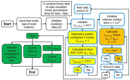
Figure 4.
Solar-driven adsorption air conditioning model algorithm flowchart [10].
3. Simulation Operating Conditions
3.1. Solar Operating Conditions
Daily hourly weather data for the hottest day instead of monthly data were used to meet the required cooling capacity (up to 2.5 kW), as well as the required solar collector size for continuous operation of the adsorption air conditioning system. This was due to the better approximation of the weather conditions throughout the year that the monthly weather data provided. The solar daily hourly and monthly data extracted from METEONORM 7.V7.32 are summed up in Table 3 and Table 4, respectively. Overall, both ambient temperatures and solar radiation levels were higher during the hottest day, as well as the ordinary days, than the monthly data. It is, therefore, more appropriate to use daily hourly data to size the solar collector.
Table 3.
Singapore hourly solar insolation on the hottest day (5 April).
Table 4.
Singapore monthly solar insolation levels and sunlight hours.
3.2. Air Conditioning Operating Temperatures
The driving temperature Tdriving (also corresponding to solar collector temperature Tcol) ranges from 70 °C to 140 °C (calculations performed in 1 °C increments). This minimum of 70 °C is linked to the selected active carbon–methanol pair, while the maximum of 140 °C is related to the methanol decomposition temperature, estimated to be around 160 °C in the presence of active carbon. The outdoor temperatures correspond to the ambient temperatures provided in Table 3. The condensing temperatures (Tcond) are 5 °C above the ambient temperatures (Tamb). For ideal comfort, the indoor temperature is fixed to 22 °C, which is well within the WHO recommendations of indoor temperature between 18 °C and 24 °C [21,22] and commonly used in various air conditioning guidelines and standards such as ASHREA [23,24]. The evaporating temperature Tevap is 7 °C below the indoor temperature and corresponds to 15 °C.
4. Results Analysis and Discussion
Figure 5 shows the predicted key performance indicators (KPIs) of the adsorption air conditioning system with the described thermal compressor. The SCP increases linearly with the driving temperature and ranges between 0.3 kW kg−1 and 1.4 kW kg−1, regardless of the time of the day. Similarly, the COP ranges between 0.35 and 0.65, but with optimal values when the driving temperatures range between 80 °C and 90 °C.
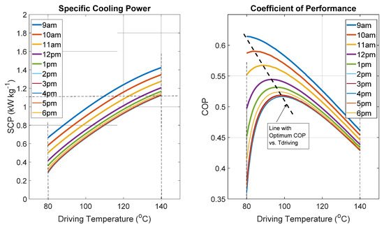
Figure 5.
SCP and COP model predictions for function of driving temperature.
The trend observed on COP vs. Tdriving is common for adsorption systems [25,26,27]. In general, with an adsorption cooling machine operating with a large spectrum of driving temperatures with fixed evaporating and condensing temperatures, the COP will exhibit a maximum value at a certain driving temperature. As driving temperature is increased, the amount of refrigerant driven off will increase, increasing the cooling energy per cycle and COP. However, beyond a certain driving temperature, the additional amount of refrigerant driven off will slow down and the additional cooling will be outweighed by the additional heat input, leading to a drop in COP. It is worthwhile pointing out that the partial trend of COP vs. Tdriving (with up-trend or down-trend only) could also be observed depending on the temperature spectrum explored in some cases [25,26,28], including at both 9:00 and 10:00 in Figure 5.
These intrinsic KPIs are established by using the hourly daily ambient temperature (Tamb) in the first instance, which corresponds to a given condensing temperature (Tcond = Tamb + 5 °C). This means that the profiles shown are isotherms (constant ambient temperature), and thus the 2 pm and 6 pm characteristics (Tamb = 33.7 °C) are identical. Based on both maximum operating temperature (140 °C) and cooling capacity (up to 2.5 kW), the minimum SCP must be around 1.1 kW kg−1, with maximum solar radiation during the day at 4 pm (1049 W m−2). The proposed system is, therefore, rated for a nominal cooling capacity of about 2.5 kW. By balancing both the effective received solar energy rate by the collector and the energy rate required by the thermal compressor (with reference to Equation (29)), both collector surface area and driving temperature are estimated. The FPSC’s required surface area is estimated to be about 17.6 m2, corresponding to a cost of EUR 8800 (Figure 6), while ETSC only needs an area of about 9.8 m2 and a cost of about EUR 7150 (Figure 7) to achieve a similar cooling capacity. The KPIs with FPSC and ETSC are shown in Table 5 and Table 6, respectively. FPSC costs about 19% more than ETSC and requires about 44% more than the ETSC area. It is, therefore, cost effective to use the selected ETSC in the proposed solar thermally driven adsorption air conditioning system.
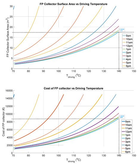
Figure 6.
Flat plate solar collector (FPSC) area and cost model predictions for function of driving temperature.
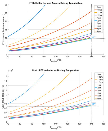
Figure 7.
Evacuated tube solar collector (ETSC) area and cost model predictions for function of driving temperature.
Table 5.
Air conditioning performance with FPTSC (Acol = 17.6 m2) on the hottest day (5 April).
Table 6.
Air conditioning performance with ETSC (Acol = 9.8 m2) on the hottest day (5 April).
In Singapore, the capital cost of a conventional air conditioning unit is estimated to be about SGD 1200 with an annual running cost (electricity and maintenance) of SGD 2335. With an average lifespan of 7 years, the total cost of an air conditioning unit in Singapore is estimated to about SGD 17,550 (~EUR 12,530).
The current adsorption air conditioning system has an estimated capital cost of EUR 8800 (~SGD 12,350). The breakdown for the major components is as follows: EUR 7150 for the 9.8 m2 evacuated tube solar collector (ETSC), EUR 600 for the pair of generators, EUR 500 for the evaporator, EUR 100 for the condenser, EUR 100 for the cooler, and EUR 350 for two water pumps [20]. The costs of the expansion valve, piping required, and auxiliaries are estimated to EUR 500. The annual running cost including maintenance and electricity is assumed to be EUR 150. In 7 years’, time, this would result in a total cost of EUR 10,550 (~SGD 14,800), which is relatively less expensive (about 16%) than a conventional air conditioning unit. The estimated capital cost for a one-off machine is about EUR 4000/kWc, which is fair given the cost of such a system (typically between EUR 3000/kWc and EUR 4000/kWc) [29,30]. Furthermore, the current adsorption air conditioning system could last 15 to 20 years. This means that the proposed system has 7 years’ payback and 7 years to 13 years of further “zero-cost cooling”.
The performance of the air conditioning system on the hottest day is shown in Table 6: both cooling capacity (between 1 kW and 2.6 kW) and COP (between 0.43 and 0.58) are well within the nominal design performance. This means there is a daily cooling energy production of 20 kWh from 41 kWh daily useful heat input, and the COP on this day is about 0.50. Furthermore, the annual cooling energy production is about 3400 kWh, and the annual solar heat input 6700 kWh, giving a seasonal COP of about 0.51. Figure 8 shows the cooling energy production and corresponding COP for each day of the year. The machine will obviously not operate every day (there are a few days with total cloud cover) or for the entire 24-h day without some form of storage. As shown in Figure 9, the typical cooling production period is only between 10:00 am and 4:00 pm. To remedy this, the evaporator will have two compartments: a chiller section for air conditioning and an ice bank section (Tevap = −5 °C). The ice is produced and stored when the cooling demand is low during the day. This ice bank could then be used for night cooling demand or daily cooling demand as a top-up, or during periods of low insolation (typically below 300 W m−2).
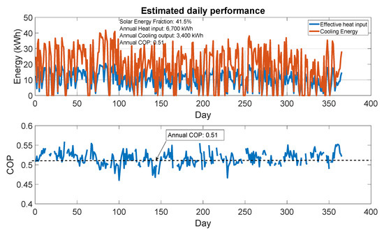
Figure 8.
Daily performance throughout the year with 9.8 m2 evacuated tube solar collector (ETSC).
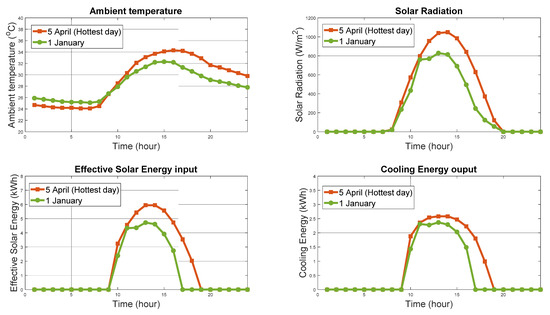
Figure 9.
Examples of hourly daily cooling production (1 January and 5 April).
5. Conclusions
The design of an adsorption air conditioning system using activated carbon–methanol as the working pair has been investigated for potential use in Singapore. A detailed and rigorous system design methodology is described. It includes:
- A physical description of the adsorption reactor (thermal compressor), which is a shell (154.4 mm OD × 1.63 mm wall thickness in stainless steel), and the micro-tube (800 micro-tubes of 1.2 mm OD × 2 mm wall thickness in stainless steel with about 2 mm layer of activated carbon and methanol refrigerant) type of heat exchanger.
- An elaboration of finite difference modelling of the adsorption reactor based on both mass and heat balances leading to the establishment of the intrinsic performance of the thermal compressor, namely, the specific cooling power (SCP) and coefficient of performance (COP) as a function of the driving temperature.
- Thermal solar collector area and cost mapping for Singapore hourly weather data on the hottest day of the year (5 April), leading to sizing and costing of the required solar collector.
- A comparison of both the flat plate solar collector (FPSC) and the evacuated tube solar collector (ETSC), leading to ETSC being identified as the most cost coeffective (19% cheaper) option with 9.8 m2 area vs. 17.6 m2 to achieve similar nominal cooling capacity (2.6 kW).
- An exploitation of the elaborated model with a 9.8 m2 ETSC to predict the hourly, daily and annual performance of air conditioning.
Overall, with the proposed adsorption air conditioning system for Singapore, a maximum cooling power of 2.6 kW and a COP of 0.43 are achieved at a maximum driving temperature of 139 °C with a 9.8 m2 ETSC on the hottest day of the year. The system has a total estimated cost of EUR 10,550 corresponding to about SGD 14,800 with 7 years’ payback time. The proposed system could last 7 to 13 more years than a conventional air conditioning unit with similar rated cooling capacity.
Author Contributions
Conceptualization, Z.T.-T. and S.J.M.; Investigation, N.N.Y.; Methodology, Z.T.-T., S.J.M. and N.N.Y.; Software, Z.T.-T., S.J.M. and N.N.Y.; Supervision, Z.T.-T.; Visualization, N.N.Y.; Writing—original draft, Z.T.-T.; Writing—review and editing, Z.T.-T. and S.J.M. All authors have read and agreed to the published version of the manuscript.
Funding
This research received no external funding.
Institutional Review Board Statement
Not applicable.
Informed Consent Statement
Not applicable.
Data Availability Statement
MATLAB® Figures as well as numerical data generated on EXCEL sheet (with embedded instructions) are attached in the open access Warwick Research Archive Portal (WRAP) and are accessible through the following link: http://wrap.warwick.ac.uk/168864/ (accessed on 28 August 2022).
Acknowledgments
The authors would like to thank both Nanyang Technological University (NTU)—Singapore and the University of Warwick—UK for supporting this project under the Overseas Final Year Project (OFYP) Scheme 2019.
Conflicts of Interest
The authors declare no conflict of interest.
Nomenclature
| Acronyms | |
| ANSI | American National Standards Institute |
| ASHRAE | American Society of Heating, Refrigerating and Air-Conditioning Engineers |
| COP | Coefficient of Performance |
| D–A | Dubinin–Astakhov |
| ETSC | Evacuated Tube Solar collector |
| FPSC | Flat Plate Solar collector |
| HEX | Heat Exchanger |
| HTF | Heat Transfer Fluid |
| ID | Inner Diameter (m or mm) |
| kWc | Kilowatt Cooling |
| LPM | Liter per minute |
| MT | Micro-Tube or Miniaturized Tube |
| OD | Outer Diameter (m or mm) |
| SCP | Specific Cooling Power (W kg−1 or kW kg−1) |
| S$ | Singapore Dollar currency |
| SS | Stainless Steel |
| SV | Solenoid Valve |
| TREX | Tubular Reactor Heat Exchanger |
| WHO | World Health Organization |
| Latin Symbols | |
| A | Area (m2) |
| c | Specific heat capacity (J kg−1 K−1) |
| D | Diameter (m) |
| G | Solar Insolation (W m−2) |
| h | Convection heat transfer coefficient (W m−2 K−1) |
| h | Specific enthalpy of refrigerant (J kg−1) |
| H | Specific enthalpy of sorption (J kg−1) |
| k1 | Linear loss coefficient (W m−2 K−1) |
| k2 | Quadratic loss coefficient (W m−2 K−2) |
| k | D–A parameter |
| KPI | Key Performance Indicator |
| L | Length (m) |
| m | Mass (kg) |
| n | D–A parameter |
| Nu | Nusselt Number |
| q | Heat rate (W) |
| Q | Heat energy (J) |
| Re | Reynolds Number |
| th | Thickness (m or mm) |
| T | Temperature ( or K) |
| UA | Overall Heat Transfer Coefficient (W K−1) |
| v | Velocity (m s−1) |
| Volumetric flow rate (m−3 s−1) | |
| x | Refrigerant uptake (kg Methanol kg−1 Carbon) |
| xo | Maximum Refrigerant uptake (kg Methanol kg−1 Carbon) |
| Greek symbols | |
| ∆ | Difference |
| € | Euro currency |
| η | Efficiency of solar collector |
| λ | Thermal conductivity (W m−1 K−1) |
| µ | Dynamic viscosity (kg m−1 s−1) |
| ρ | Density (kg m−3) |
| Subscripts | |
| amb | Ambient |
| c | Carbon |
| con | Condensation or Condenser |
| col | Solar collector |
| cool | Cooling |
| driving | Driving temperature of adsorption system |
| evap | Evaporation or Evaporator |
| f | Fluid in liquid form |
| HP | High Pressure |
| i | Inner |
| in | Into HEX |
| m | Methanol |
| LP | Low Pressure |
| o | Outer |
| opt | Optimum |
| out | Out of solar collector |
| p | Pressure |
| sat | Saturation |
| sup | Superheated vapor |
| t | Tube or Micro-Tube |
| v | Volume |
| w | Stainless Steel wall between carbon and HTF |
References
- Asia, C.N. Air Conditioning for All? Hotter World Faces Risk of ‘Cooling Poverty’. Available online: https://www.channelnewsasia.com/world/climate-change-air-conditioning-hotter-world-risk-8603062019 (accessed on 13 September 2019).
- Singapore, E.M.A. Singapore Energy Statistics 2018. Available online: https://www.ema.gov.sg/Singapore_Energy_Statistics.aspx (accessed on 13 September 2019).
- Chua, K.J.; Chou, K.S.; Yang, W.M.; Yan, J. Achieving better energy-efficient air conditioning—A review of technologies and strategies. Appl. Energy 2013, 104, 87–104. [Google Scholar] [CrossRef]
- Electricity Tariff Revision for the Period of 1 July to September 2019. Available online: https://www.spgroup.com.sg/wcm/connect/spgrp/ (accessed on 4 August 2021).
- Smart ENVi Series, Daikin Split Air Conditioning Units, Catalogue 2019; Daikin: Osaka, Japan, 2019.
- Air-Con-System-Efficiency-Primer-A-Summary. Available online: https://www.nccs.gov.sg/files/docs/default-source/default-document-library/air-con-system-efficiency-primer-a-summary.pdf (accessed on 4 August 2021).
- Chapter 14 climatic design information. In ASHRAE-Handbook-Fundamentals; ASHRAE: Atlanta, GA, USA, 2019.
- Kalkan, N.; Young, E.; Celiktas, A. Solar thermal air conditioning technology reducing the footprint of solar thermal air conditioning. Renew. Sustain. Energy Rev. 2012, 16, 6352–6383. [Google Scholar] [CrossRef]
- Weiss, W.; Spörk-Dür, M. Global Market Development and Trends 2021: Detailed Market Figures 2022; Report—IEA Solar Heating & Cooling Programme; SHC: Cedar, MI, USA, 2022. [Google Scholar]
- Yande, N.N.G. Thermal Adsorption Air Conditioning: Case Study of Singapore; Project Report; Nanyang Technological University: Singapore; University of Warwick: Coventry, UK, 2019. [Google Scholar]
- Metcalf, S.J.; Tamainot-Telto, Z.; Critoph, R.E. Novel compact sorption generators for heat pump applications, paper no. P5-49. In Proceedings of the IEA—Heat Pump Conference, Zurich, Switzerland, 22 May 2008. [Google Scholar]
- Metcalf, S.; Tamainot-Telto, Z.; Critoph, R. Application of a compact sorption generator to solar refrigeration: Case study of Dakar (Senegal). Appl. Therm. Eng. 2011, 31, 2197–2204. [Google Scholar] [CrossRef]
- Metcalf, S.; Critoph, R.; Tamainot-Telto, Z. Optimal cycle selection in carbon-ammonia adsorption cycles. Int. J. Refrig. 2012, 35, 571–580. [Google Scholar] [CrossRef]
- WKays, M.; London, A.L. Compact Heat Exchangers, 3rd ed.; McGraw-Hill: New York, NY, USA, 1984; ISBN 0-07-033418-8. [Google Scholar]
- Holman, J. Heat Transfer, 10th ed.; McGraw-Hill: New York, NY, USA, 2010; ISBN 978-007-126769-4. [Google Scholar]
- Reuck, K.M.D.; Craven, R.J.B. Methanol; Blackwell Scientific: Oxford, UK, 1993; ISBN 9780632023790. [Google Scholar]
- Turner, L.H. Improvement of Activated Charcoal-Ammonia Adsorption Heat Pumping/Refrigeration Cycles: Investigation of Porosity and Heat/Mass Transfer Chacteristics. Ph.D. Thesis, University of Warwick, Coventry, UK, 1992. [Google Scholar]
- Critoph, R.E. Evaluation of alternative refrigerant—Adsorbent pairs for refrigeration cycles. Appl. Therm. Eng. 1996, 16, 891–900. [Google Scholar] [CrossRef]
- Critoph, R.E. Adsorption refrigerators and heat pumps. In Carbon Materials for Advanced Technologies; Burchell, T.D., Ed.; Elsevier: Amsterdam, The Netherlands, 1999; Chapter 10; pp. 303–340. ISBN 0-08-042683-2. [Google Scholar]
- SolarBayer. 2018. Available online: https://www.solarbayer.com/ (accessed on 17 August 2019).
- WHO. Health impact of low indoor temperatures. In Proceedings of the WHO Meeting, Copenhagen, Denmark, 11–14 November 1985. [Google Scholar]
- WHO Housing and Health Guidelines 2018; WHO: Geneva, Switzerland, 2018; ISBN 978-92-4-155037-6.
- ANSI/ASHRAE Standard 55-2017; Thermal Environmental Conditions for Human Occupancy. ASHRAE: Atlanta, GA, USA, 2017; ISSN 1041-2336.
- ANSI/ASHRAE Addendum d to ANSI/ASHRAE Standard 55-2017; Thermal Environmental Conditions for Human Occupancy. ASHRAE: Atlanta, GA, USA, 2020; ISSN 1041-2336.
- Wang, R.Z. Performance improvement of adsorption cooling by heat and mass recovery operation. Int. J. Refrig. 2001, 2, 602–611. [Google Scholar] [CrossRef]
- Critoph, R.E.; Metcalf, S.J. Specific cooling power intensification limits in ammonia–carbon adsorption refrigeration systems. Appl. Therm. Eng. 2004, 24, 661–678. [Google Scholar] [CrossRef]
- Habib, K.; Saha, B.B.; Koyama, S. Study of various adsorbent–refrigerant pairs for the application of solar driven adsorption cooling in tropical climates. Appl. Therm. Eng. 2014, 72, 266–274. [Google Scholar] [CrossRef]
- Henning, H.; Häberle, A.; Guerra, M.; Motta, M. Solar Cooling and Refrigeration with High Temperature Lifts—Thermodynamic Background and Technical Solution. Available online: https://www.researchgate.net/publication/268359467 (accessed on 30 July 2022).
- Renewables 2015 Global Statue Report, REN21. Available online: https://www.ren21.net/wp-content/uploads/2019/05/GSR2015_FullReport_English.pdf (accessed on 4 August 2021).
- Roumpedakis, T.C.; Vasta, S.; Sapienza, A.; Kallis, G.; Karellas, S.; Wittstadt, U.; Tanne, M.; Harborth, N.; Sonnenfeld, U. Performance Results of a Solar Adsorption Cooling and Heating Unit. Energies 2020, 13, 1630. [Google Scholar] [CrossRef] [Green Version]
Publisher’s Note: MDPI stays neutral with regard to jurisdictional claims in published maps and institutional affiliations. |
© 2022 by the authors. Licensee MDPI, Basel, Switzerland. This article is an open access article distributed under the terms and conditions of the Creative Commons Attribution (CC BY) license (https://creativecommons.org/licenses/by/4.0/).