Abstract
The spark ignition engine is a complex multi-domain system that contains many variables to be controlled and managed with the aim of attending to performance requirements. The traditional method and workflow of the engine calibration comprise measure and calibration through the design of an experimental process that demands high time and costs on bench testing. For the growing use of virtualization through artificial neural networks for physical systems at the component and system level, we came up with a likely efficiency adoption of the same approach for the case of engine calibration that could bring much better cost reduction and efficiency. Therefore, we developed a workflow integrated into the development cycle that allows us to model an engine black-box model based on an auto-generated feedfoward Artificial Neural Network without needing the human expertise required by a hand-crafted process. The model’s structure and parameters are determined and optimized by a genetic algorithm. The proposed method was used to create an ANN model for injection parameters calibration purposes. The experimental results indicated that the method could reduce the time and costs of bench testing.
1. Introduction
To meet climatic and performance requirements, the engine mechanisms become more complex each year (Dual Variable Valve Timing, variable valve lift, and direct injection with multiple pulses). Consequently, more development time and more accurate engine calibration are necessary. However, this is against the automotive market demand that requires more new technologies in less time.
The engine calibration process consists of adjusting Engine Control Unit (ECU) parameters to improve the efficiency and performance of the engine to achieve goals such as reducing fuel consumption, reducing emissions of exhaust gas into the environment to meet local emissions regulations, and improving engine power, durability and drivability. Controlling an engine is one of the most complex tasks for systems control engineers and researchers around the world because of the large number of variables to control, such as engine speed, engine torque, spark ignition timing, fuel injection timing, air intake, air–fuel ratio (AFR) [1], and also because these variables are dependent on each other. Moreover, besides the increase in engine calibration effort, engineers in the automotive sector constantly face a decrease in the development process time.
To overcome these problems, several types of research have been conducted in recent years to optimize the tuning development process using a model-based method [2]. The main advantage of using model-based methods in the tuning development process is that it enables the calibration engineer to evaluate parameters in a multi-dimensional space without additional testing.
Figure 1 shows the workflow for experimental engine modeling with test benches that consist, basically, of acquiring and preparing engine data, modeling the engine by using a model-based method, and finally, analyzing and validating the engine model. Among the type of model-based methods, the Artificial Neural Networks (ANN) have demonstrated their effectiveness in several works [3,4,5,6] thanks to their power to approximate and the capacity of their ability to adapt to a wide variety of non-linearities. However, the accuracy of an ANN model lies, in part, on the ANN architecture parameters or hyperparameters, and finding the ideal ANN architecture for a given problem remains empirical. Therefore, some researchers [7,8,9] propose an approach based on a meta-heuristic algorithm in order to create optimized ANN architecture.

Figure 1.
Workflow for experimental engine modeling with test benches.
Meta-heuristic algorithms aim to provide an excellent solution to an optimization problem with less computational effort than calculus-based methods or simple heuristics can [10]. Although meta-heuristics algorithms can be used to solve almost all optimization problems, there is a wide variety of them. An algorithm can perform better on one type of problem and worse on another.
Absalom et al. [11] have analyzed, based on the same set of benchmark problems, the performance of twelve meta-heuristics algorithms, which are genetic algorithms (GA) [12], particle swarm optimization (PSO) [13], ant colony optimization [14], symbiotic organisms search [15], cuckoo search [16], firefly algorithms [17], artificial bee colony [18], bat algorithms [19], differential evolution (DE) [20], flower pollination algorithms [21], invasive weed optimization [22], and BeeA [23]. Among these algorithms, those which performed better across all the test problems were DE, PSO, and GA.
In the current paper, we propose a practical and versatile method of modeling engines using a feedforward artificial neural network whose architecture is optimized by GA.
The contribution of this study is the development of a versatile method for modeling an engine black-box model based on an auto-generated feedfoward Artificial Neural Network for tuning development purposes, without needing the human expertise required by a hand-crafted process. Therefore, we propose an improved ANN to build a spark-ignition engine model. The model’s structure and parameters are determined and optimized by a genetic algorithm. A specific project experiment verifies the effectiveness of the method. The experimental results indicates that the technique could reduce the time and costs of bench testing. The results have specific guiding significance for the design of the internal combustion engine.
2. Related Work
2.1. Model-Based Engine Design
Engine modeling type can be divided into two main categories, which are the theoretical and experimental modeling, also called white-box and black-box models, respectively.
White-box models are suitable when physical laws and parameters are known [24]. Thermodynamic, chemical, heat transfer, and fluid dynamic models based on the numerical calculation can predict the engine dynamics as intake mass flow, combustion efficiency, engine heat release, torque generation, fuel consumption, and emission of pollutants through multiple dimensions equations.
Black-box models are based on measurement to establish, through an identification model, the relationship between input and output signal measured. However, in many practical applications [25,26,27], the combination of white-box and black-box models are used, resulting in two other engine modeling sub-categories, which are light-gray-box models and dark-gray-box models, as shown in Table 1.

Table 1.
Different kinds of mathematical process models.
In 2015, Shamekhi et al. [28] introduced a new method to improve a well-known white-box model, the mean value model (MVM). Those models provide an approximate mathematical relation of an engine by describing the time development of its physical variable dynamically over periods [29]. To improve the MVM accuracy, they proposed a gray-box model named the Neuro-MVM, a combination of Neural Networks with MVM. Their model was designed to predict the torque, CO, and NOx, by receiving the ambient pressure and temperature, throttle angle, air/fuel ratio, the crank angle of spark advance, the external load, and the initial speed. The study showed that not only does the Neuro-MVM achieve great precision in predicting their model outputs, which are speed, but the model also has more reliability than a Neural Network.
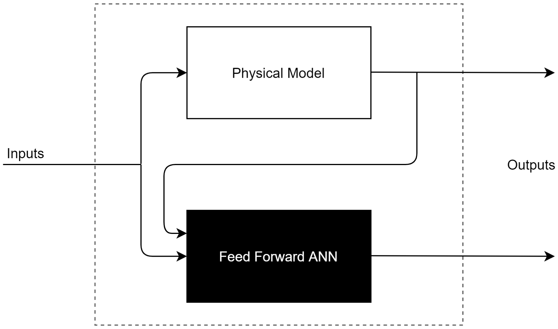
In other works conducted by Nazoktabar et al. [30] to develop a multi-zone model for a Homogeneous Charge Compression Ignition Engine, they used a gray-box model which was able to predict the indicated mean effective pressure, the crank angle for 50 percent burned, carbon monoxide, and the total hydrocarbon, with average errors of 1.2 CAD, 0.4 bar, 10 PPM, and 394 PPM, respectively. As shown in Figure 2, this model consists of two physical models and two black-box models, where the white-box model’s outputs are used as the mean input to the ANN models.
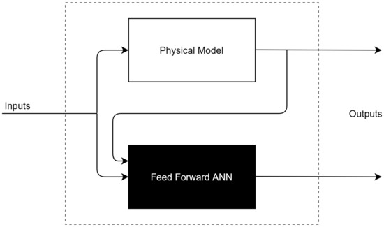
Figure 2.
Combination of physical and black box model.
Black-Box Model
Black-box models are used for SI Engine calibration purposes, either because it is impossible to model some engine parts theoretically due to the lack of knowledge about some parameters, or when the construction time of a non-linear physical model is incompatible with engine development time, making the white-box modeling impracticable [31]. So, given the importance of Black-box models, building accurate models attracted the research community’s interest in recent years.
In 1996, a study conducted by Nicolao et al. [32] investigated the effectiveness of using the black-box model to model the volumetric efficiency of an Internal Combustion Engine. For this purpose, they compared the additive, polynomial, and two Neural Network models, the radial basis function, and the multi-layer perceptrons. The study showed that these black-box models could be successfully used to describe the volumetric efficiency. However, the radial basis function (RBF) neural network and the multi-layer perceptrons (MLP) method performed better than the additive and polynomial models.
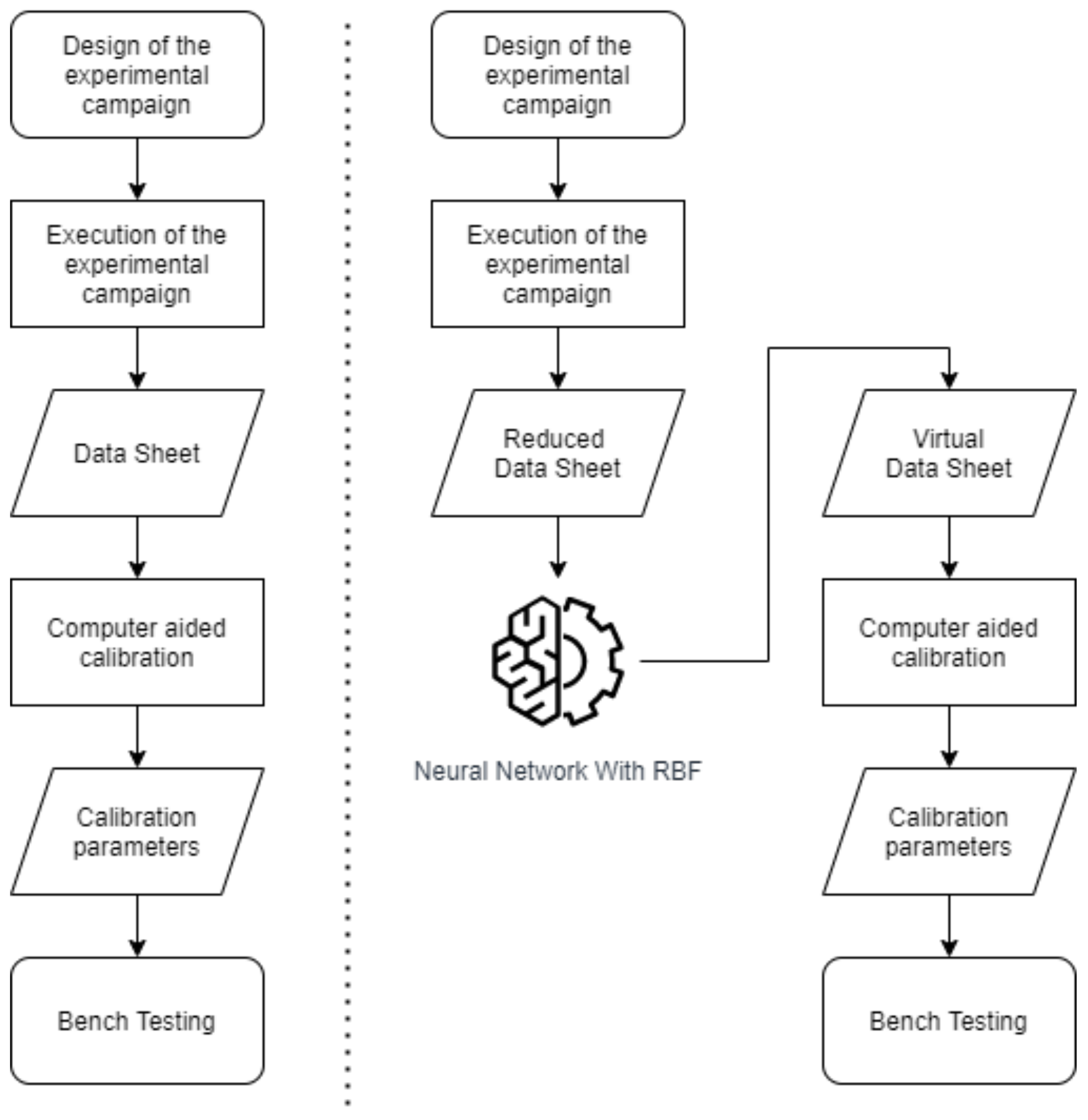
Another study conducted by Francesco et al. in 2019 [33] was proposed, as shown in Figure 3, an ANN-based method for improving the calibration methodology by reducing bench test activity, acquiring few data. The main advantage of this method is that with these few data, more detailed virtual engine data can be generated for calibration by using an RBF Neural Network. The proposed methodology was tested by estimating the volumetric efficiency and showing that acceptable calibration performance was reached, even after reducing by 60% experimental data commonly acquired for calibration.

Figure 3.
Scheme of the improved calibration methodology.
In addition to the ANN engine modeling method, the Support Vector Machine (SVM) has been investigated for modeling an Internal Combustion Engine used to predict engine performance and emissions [34,35]. The SVM algorithm is a machine learning method, which was introduced in 1963 by Vladimir N. Vapnik and Alexey Ya. Chervonenkis. SVMs are used as supervised learning methods for regression, classification, and outlier detection. For this reason, they can be used for complex modeling relationships between input and output without a direct physical understanding of the system. In 2020, Norouzi et al. [36] used the SVM to develop a Model Oder Reduction algorithm to predict the steady-state of brake mean effective pressure and NOx emission of a medium-duty diesel. They compared their approach with a two-layer (three neurons in the hidden layer) feed-forward back-propagation neural network trained with the Levenberg–Marquardt training method. This comparison shows that the SVM approach is more accurate and faster than the ANN approach. However, it is essential to note that the ANN architecture (the number of layers and neurons) used for this comparison was chosen based on another similar study [37,38].
2.2. Artificial Neural Network Architecture Optimization
ANNs are generally defined by their kind of neuron, architecture, learning algorithm, and recall algorithm [39]. The ANN architecture comprises an input layer, one or more hidden layers, and an output layer, which describes how neurons are connected and can be classified into two major categories: feedforward and feedback architecture. Depending on the problem to be solved, a suitable number of hidden layers and neurons in each layer has to be set, since it affects the ANN performance. However, there is no theory-based method to find this value, and therefore, meta-heuristics algorithms have been successfully used to find an optimal ANN architecture configuration.
In 2010, Carvalho et al. [8] investigated four optimization algorithms (the Generalized Extremal Optimization, the Variable Neighborhood Search, Simulated Annealing, and canonical genetic algorithm) to propose a new adaptable method for optimizing a feedforward neural network architecture. The ANN’s architecture parameters that were optimized were: the function activation (Tanh, sigmoid, log, Gaussian), the hidden layers (from 1 to 3), and the neurons in each hidden layer (from 1 to 32). Their study was conducted based on standard benchmark data sets from the machine learning repository of the University of California Irvine. It showed that the Variable Neighborhood Search and the Genetic Algorithm performed better than the others. Despite the computational cost, this methodology was more efficient than the trial and error method for designing an ANN architecture.
The following section presents our proposed methodology for modeling an Internal Combustion Engine using a Feedforward ANN and the Genetic Algorithm.
3. The Proposed Methodology
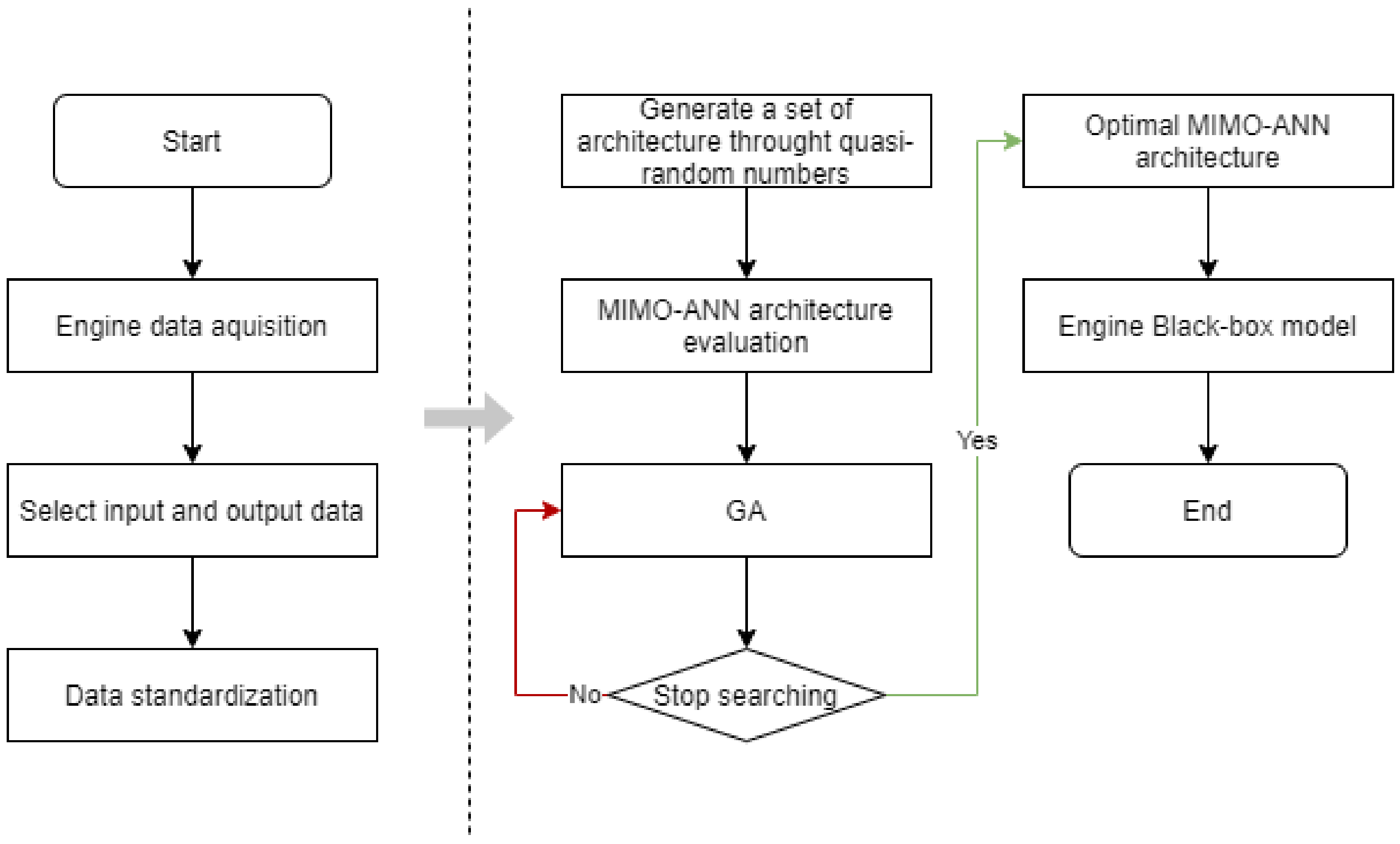
The proposed methodology in this paper is described in Figure 4. It aims to present an adaptable method to enhance, using the genetic algorithm, the accuracy of a feedfoward ANN engine black-box model for tuning development purposes. Therefore, we begin by defining the ANN architecture’s parameters to be optimized. In this paper, we will consider the findings shown in Table 2. The following parameters are the transfer function, the layer number, the number of nodes in each layer, and the epoch number.

Figure 4.
The process of virtual modeling for a spark ignition engine through ANN + GA.
Table 2.
ANN architecture properties optimized.
Then, the meta-heuristic algorithm generates an initial possible solution set (population) with a quasi-random number generator (QRNG). The use of QRNGs was motivated by the property that these generators have to minimize the discrepancy between the distribution of the generated points, enabling them to present better results in solving optimization problems using GA compared to pseudo-randomly generated sequences [40].
Next, each ANN architecture of the initial population is evaluated using the test bench data. These data are represented by a matrix . Since the signals can have different orders of magnitude, the matrix is standardized in an interval to minimize the error during ANN training using Equation (1).
Once the data are standardized, the ANNs are fed with the input signals to be trained with a supervised learning algorithm, and their performances are evaluated. The performance of ANNs is usually assessed using error metrics. The most common metrics are the Mean Absolute Error (MAE), the Mean Square Error (MSE), the Root Mean Square Error (RMSE), and the Mean Absolute Percent Error (MAPE) given by the Equations (2)–(5), respectively, where n represents the number of data, y the effective value, and t the value estimated by the ANN [41].
After evaluating all architectures, the next generation of architectures is generated by the meta-heuristic algorithm, and so on, until the optimum architecture is found.
3.1. Feedforward Artificial Neural Network
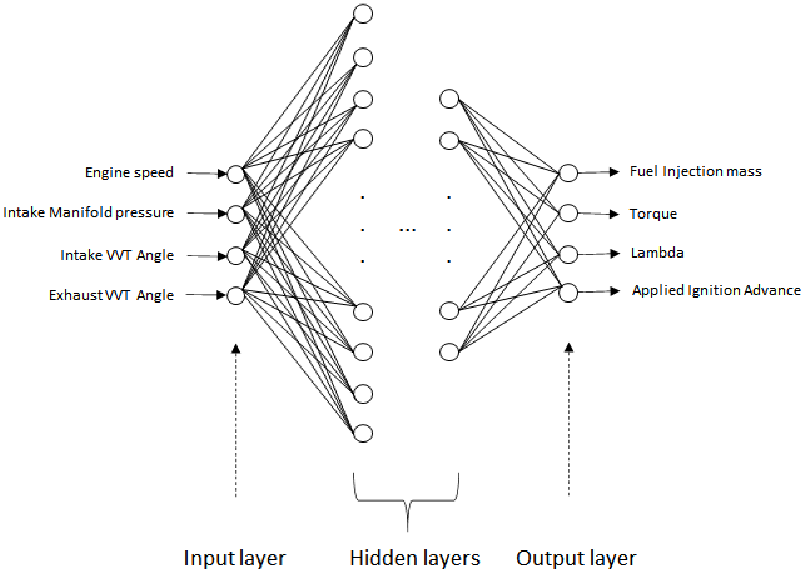
The Multilayer feedforward network, most commonly called Multilayer Perceptron (MLP), is a class of neural networks that are characterized, as represented in Figure 5, by an input layer, one or more hidden layers, and an output layer. In the MLP, the input signal in the input layer passes through the network, neurons by neurons from left to right, in a forward direction. Neurons are a non-linear function given by (6), where , and are the activation function, the variables, and synaptic weights, respectively. Table 3 shows the equations of the activation function investigated in this paper.
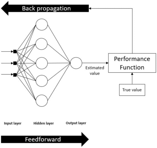
Figure 5.
MLP Feedfoward Neural Network Architecture.
Table 3.
Activation Functions.
Several complex problems have been solved by training MLPs in a supervised manner with an error back-propagation learning algorithm that occurs in two steps. The first step consists of applying, in the input layer, a set of input data that propagate, layer by coating from left to right, through the network to produce a set of outputs. During this step (the forward pass), all synaptic weights of the network are fixed. In the second step, an error signal calculated by the Equation (7) propagates backward from right to left to adjust synaptic weights to make the network response move closer to the desired response.
In this study, to train the MLP, two supervised algorithms have been investigated: the Levenberg–Marquardt backpropagation and the Bayesian regularization backpropagation.
3.1.1. Levenberg–Marquardt Backpropagation
The Levenberg–Marquardt algorithm is a well-known method used in non-linear least-squares problems [42], in which, given a set of m empirical pairs of independent and dependent variables, the parameters of the model curve can be found, so that the sum of the squares of the deviations is minimized:
which is assumed to be non-empty.
The Levenberg–Marquardt method is the combination of the gradient descent method and the Gauss–Newton method. In the first one, the sum of the squared errors is reduced by updating the parameters in the steepest-descent direction. In the last one, the sum of the squared errors is reduced by assuming the least-squares function is locally quadratic in the parameters and finding the minimum of this quadratic [43].
Therefore, the Levenberg–Marquardt algorithm refers to a variation of quasi-Newton’s method designed for minimizing functions to approach second-order training speed without needing to compute the Hessian matrix. When the cost function is a sum of squares, which is a cost widely used in training feedforward networks, the Hessian matrix can be approximated as , and the gradient can be computed as . Note that J is the Jacobian matrix that contains the first derivatives of the network errors related to the weights and biases, and e is a vector of network errors. The Levenberg–Marquardt algorithm uses these approximation to the Hessian matrix in the following Newton-like update: . Note that when the scalar is equal to zero, is just Newton’s method, using the approximate Hessian matrix.
This is very well suited to neural network training, where the performance index is the mean squared error. If each target occurs with equal probability, the mean squared error, given by , is proportional to the sum of squared errors over the Q targets in the training set.
The basic algorithm for the numerical optimization of a performance index is
where is the weight matrix and is the negative of the gradient.
Let us assume that is a sum of squares function:
then, the element of the gradient would be
The key step in the Levenberg–Marquardt algorithm is the computation of the Jacobian matrix
where the Jacobian matrix is given by
The next step consists of figuring out the Hessian matrix, in which the the element of the Hessian matrix would be
Then, the Hessian matrix can be approximated as
3.1.2. Bayesian Regularization Backpropagation
First of all, Bayesian inference is a method of statistical inference in which Bayes’ theorem is used to update the probability of a hypothesis as more evidence or information becomes available. It allows the posterior probability to be derived as a consequence of two antecedents: a prior probability and a “likelihood function” derived from a statistical model for the observed data.
where H stands for any hypothesis, is the prior probability, E is the evidence, is the posterior probability, is the probability of observing E given H, and is sometimes termed the marginal likelihood or “model evidence”.
Bayesian regularization minimizes squared errors and weight and then determines the correct combination to produce a network that generalizes well.
When applying Bayes’ theorem to ANN, the probability function is defined as:
where:
D represents the set of data used during training,
x is a vector that contains all weights,
A represents the architecture class of the network, and
, are parameters associated with the density probabilities .
The performance index used by the algorithm to train the ANN is given by the square sum of the weights of the network and the average sum of the network errors.
where,
and
This index is then minimized using the Levenberg–Marquardt algorithm and the parameters and , estimated by the density probability to achieve convergence. This procedure makes the Bayesian regularization backpropagation slower compared to Levenberg–Marquardt backpropagation, but more robust and less susceptible to suffering from overfitting [44].
3.2. ANN Architecture Optimization by Genetic Algorithm
Several engine black-box models have to be built during a tuning development process. Then, it os necessary to find a suitable ANN architecture to ensure acceptable accuracy.
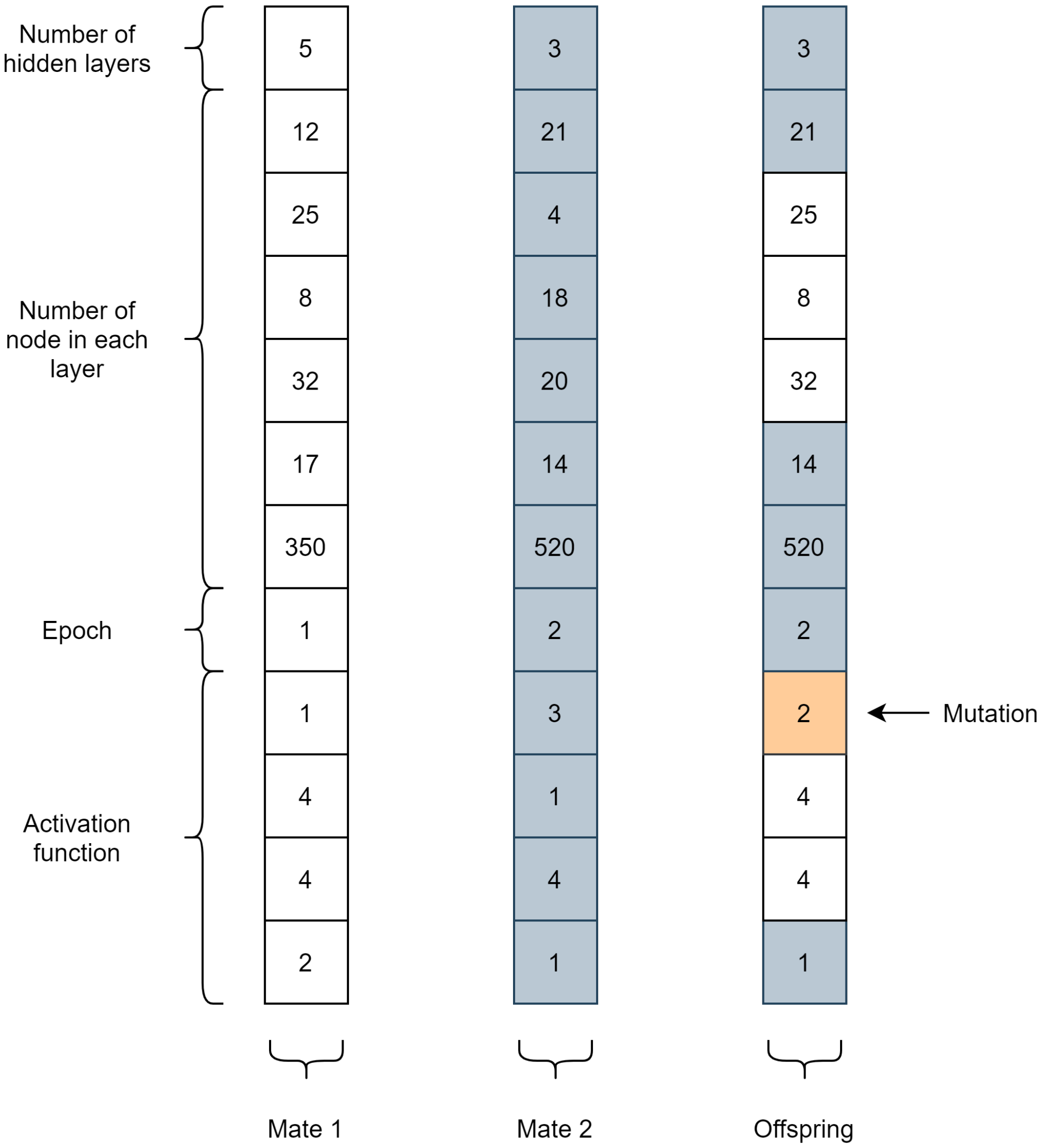
The optimization process using GA, as shown in Algorithm 1, begins by randomly generating the initial individual with the Halton Quasi-Random Point Set. An individual is represented by a set of genes that are the information that defines him, as shown in Figure 6. For the representation of the genes, decimal coding was used, where the numbers of layers, neurons, and epochs receive their corresponding values. Each of the activation functions of the set were associated, respectively, with the natural numbers in the set .
| Algorithm 1 Genetic Algorithm Pseudo-Code |
1: S← Population size 2: Define the percentage of the population that remains for the next generation 3: Define the mutation rate 4: Generate an initial individuals through Halton quasi-random set 5: while individual <S do 6: Evaluate the fitness of each individual 7: end while 8: ← The best individual 9: ← The best fitness 10: while stopping criteria are not met 11: Rank selection 12: Crossover 13: Individuals ← offspring 14: Mutation 15: Best ← Best Individual 16: if Best ≥ 17: ← Best 18: end if 19: end while 20: Return ← |
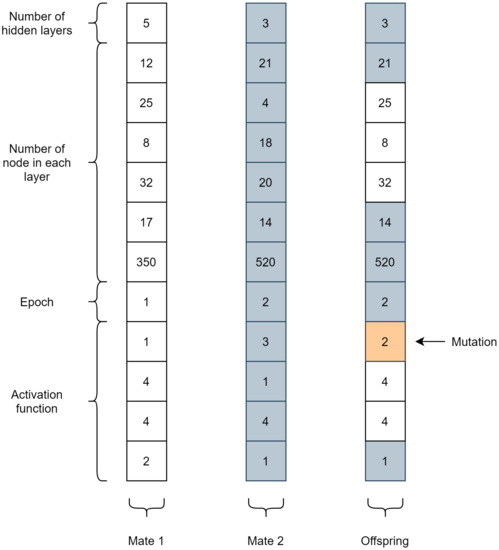
Figure 6.
Example of genes of two mates and their offspring.
Each individual, an ANN architecture, represents a possible solution for the engine modeling problem and has obtained its fitness. Since we analyze the ANNs performance using the Mean Squared Error (MSE) and ≥ 0, the fitness of each individual can be defined by:
The next step consists of selecting the individuals who will perform the crossover. The selection method implemented in this study is the rank selection, where, after sorting the individuals based on their fitness, they receive a rank n, n∈ {}, where N is the population size. The individual with the best fitness receives N, the worst receives 1, and then the likelihood of an individual i to be selected is given by:
This selection method is robust, maintaining constant pressure in the evolutionary search, but leads to a slow convergence [45].
Once the parents are selected, the offspring are generated using the crossover and mutation operator. The new individuals’ fitness is evaluated, and the best unique individuals replace the worst individuals in the population.
4. Experimental Setup
The engine calibration is performed based on data generated from engine bench tests. Some of these tests take weeks to complete. Therefore, given a calibration task, modeling the engine bench test parameters effectively from reduced data could help reduce the project time, eliminating the need to generate more data. To perform the experiment, we chose the engine’s model in Figure 7. This model’s parameters were used to calibrate the injection parameters, in which the bench test took around five weeks.
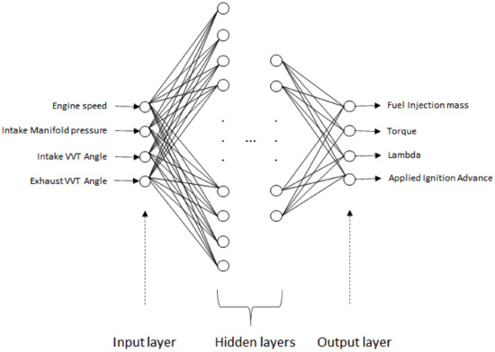
Figure 7.
ANN architecture.
At the engine test bench, we performed a data acquisition of a 1.0 L three-cylinder engine with the following operation points: Engine speed from 1000 rpm to 5800 rpm, intake and exhaust Variable Valve Timing (VVT) from minimum to maximum angles. A slow dynamic ramp of intake manifold pressure was performed at each condition from 200 hPa to 1000 hPa to measure all engine fields. The test bench automation system controlled the ignition spark angle to give CA50 = 8° (Best Consumption) or the minimum value that respect knock and cylinder pressure engine limits. The bench automation system controlled the fuel injection that gives lambda one or minimum fuel enrichment to respect the exhaust temperature engine limit. This dynamic acquisition allows the test time to be considerable.
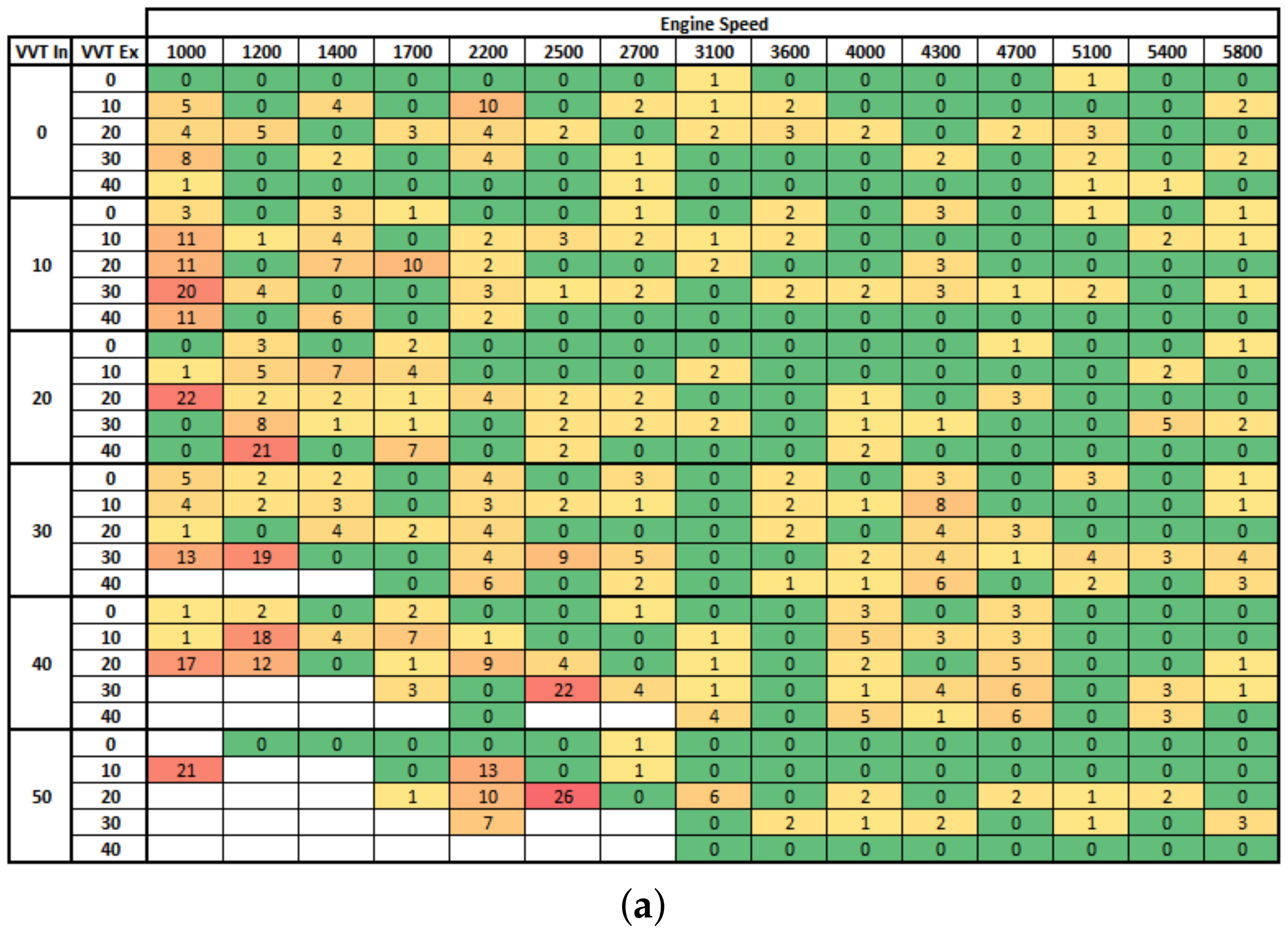
The Figure A1 below shows the acquisition points overview, where each “x” point represents about 43 acquisition points of manifold pressure from 200 hPa to 1000 hPa in steps of 20 hPa. Some points, in yellow, were not recorded due to engine combustion instability, in the form of low engine speed and extreme VVT positions. A total of 16,627 points was recorded, quantifying the entire engine field as a function of engine speed, manifold pressure, and VVT angles.
To evaluate the artificial neural network learning precision and its accuracy in modeling the engine’s dynamic, two input files were created with 65% and 43% of total acquisition data. To build the ANNs models, each of these data sets (65% and 43% of total acquisition data) was split into 75% for training, 10% for validation to avoid overfitting, and 15% for testing when using the Levenberg–Marquardt backpropagation algorithm. However, when using the Bayesian regularization backpropagation algorithm, the data split was 85% for training, 0% for validation because of the lack of need for validation data, since it is difficult to overtrain and overfit using this algorithm [46], and 15% for testing. The objective was to calculate the percentage of points with error within the criterion of acceptance of estimation errors for engine calibration purposes, according to Table 4.
Table 4.
Model validation criteria.
Since the tests performed on the test bench are always in standard conditions of intake air temperature [25 °C] and coolant temperature [90 °C], it was not considered input. The following parameters were used, as shown in Figure 7, as input for the ANN model: Engine Speed, Intake Manifold Pressure, Intake VVT Angle, and Exhaust VVT Angle.
One of the challenges when performing optimization with GA is setting the parameters. The population size, for example, affects the quality of the solution and the computation time [47]. In other words, a large population leads to more computation time, while a too-small population leads to a poor solution. Due to the time constraints in the engine turning development process, the search for an optimal ANNs architecture by GA must be performed in a tolerable time. To meet this performance and computational cost tradeoff, the genetic algorithm was configured for 50 individuals per generation to optimize the ANN architecture. The percentage of individuals remaining for the next generation was 50%, and the mutation rate was set to 8%. All the simulations and results below were performed on a notebook with 32 GB of ram and an intel i5-6446HD processor that clocked at 3.08 GHz. Due to the processing time, the optimization of the architectures using the Levenberg–Marquardt backpropagation training algorithm was performed over 16 generations and five generations for optimization of the architectures using the Bayesian regularization backpropagation as a training algorithm.
5. Experimental Results
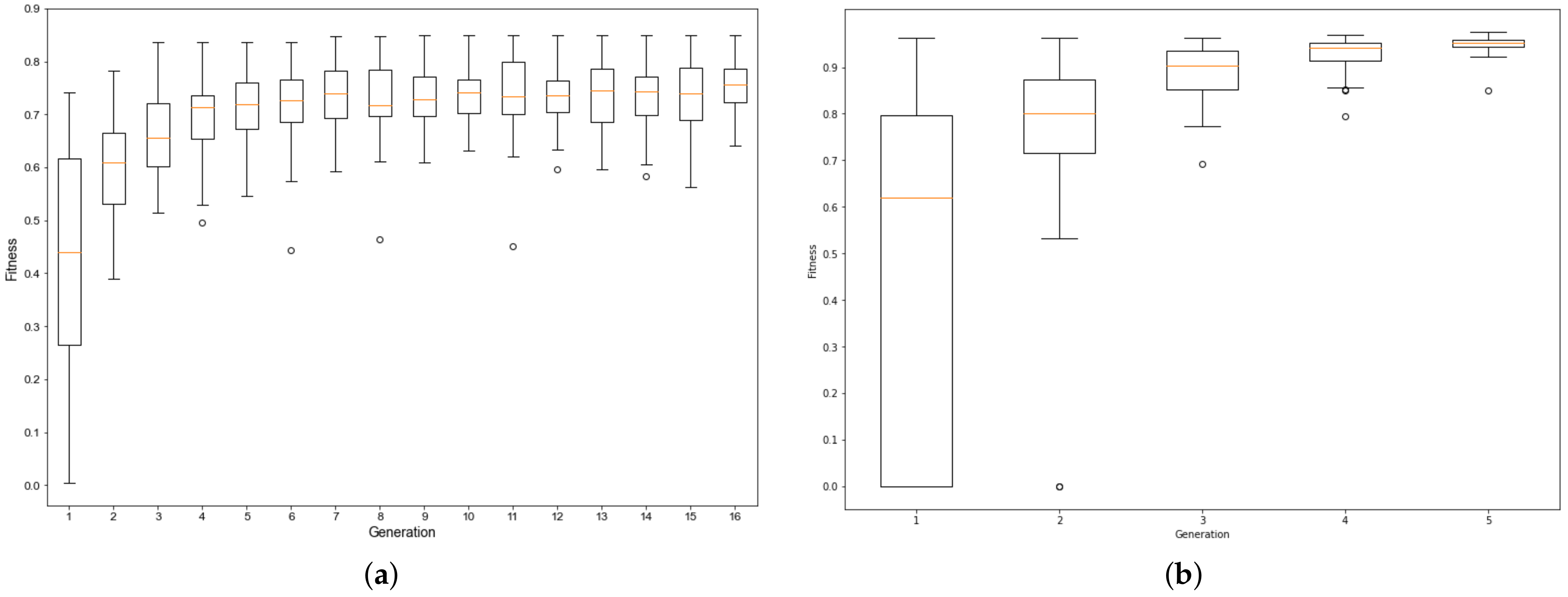
Firstly, we can see the performance of fitness evolution training of integrated ANN and GA. This shows us the best method in terms of the best configuration and performance in the training process. Since we have a vast amount of architecture which are used in training, the best statistical tool for analysis is the box plot or boxplot (also known as a box and whisker plot). This is a chart often used in descriptive data analysis, which visually shows the distribution of numerical data and skewness by displaying the data quarterlies (or percentiles) and averages. Figure 8a,b present, respectively, the fitness evolution training of two ANN, Levenberg–Marquardt and Bayesian regularization backpropagation, and using GA ranking selection method for both cases.

Figure 8.
Box plot of the fitness evolution training ANN with: (a) Levenberg–Marquardt backpropagation, (b) Bayesian regularization backpropagation.
Figure 8a is a boxplot graph that shows the fitness evolution of trained architectures using the Levenberg–Marquardt backpropagation algorithm. It might be observed that there was stabilization in the dispersion of the fitness of individuals from the fifth generation onwards, with the greatest fitness within those generations being obtained in the ninth generation, with fitness equal to . The greatest dispersion of fitness was observed in the initial generation, where the worst configuration found had a fitness equal of . In contrast, the best configuration within that generation had fitness equal to .
Figure 8b is a boxplot graph that shows the fitness evolution of the architectures trained using the Bayesian regularization backpropagation algorithm. There is a convergence trend from the fifth generation, where the best individual had fitness equal to . The greatest dispersion of fitness using this algorithm was observed in the initial generation, where the worst individual had fitness equal to . In contrast, the best individual had fitness equal to .
Table 5 shows the best ANN configuration found for each training algorithm, the fitness, and the MSE (Mean Square Error) of the ANNs in these configurations. Throughout the text, the first algorithm refers to Levenberg–Marquardt, and the second is referred to as Bayesian-Regularization. The numbers of layers equal to five, and the number of neurons are, respectively, for the first algorithm and for the second algorithm. The first algorithm takes 25 h and 12 min to complete the 16 generations, whereas the second algorithm takes 203 h and 43 min to complete the 5 generations. In terms of the run time execution, the first algorithm is shown to have a better performance. However, the results show, according to the MSE, that the Bayesian regularization is the one that that fits the data better.
Table 5.
The best configuration found for each training algorithm.
Figure 9a,b present the histogram of errors and the regression of the best ANN configuration during the training phase, respectively, using the Levenberg–Marquardt backpropagation. These graphs show that the neural network correlated the input variables of the network very well with the output variables, since the general regression was . It is also observed by the histogram of errors that the vast majority of errors were close to 0, showing that the algorithm was effective at minimizing the performance index based on the adjustment of the ANN weights; that is, learning.
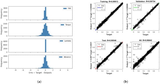
Figure 9.
(a) Histogram of errors and (b) regression during ANN training using the Levenberg–Marquardt backpropagation.
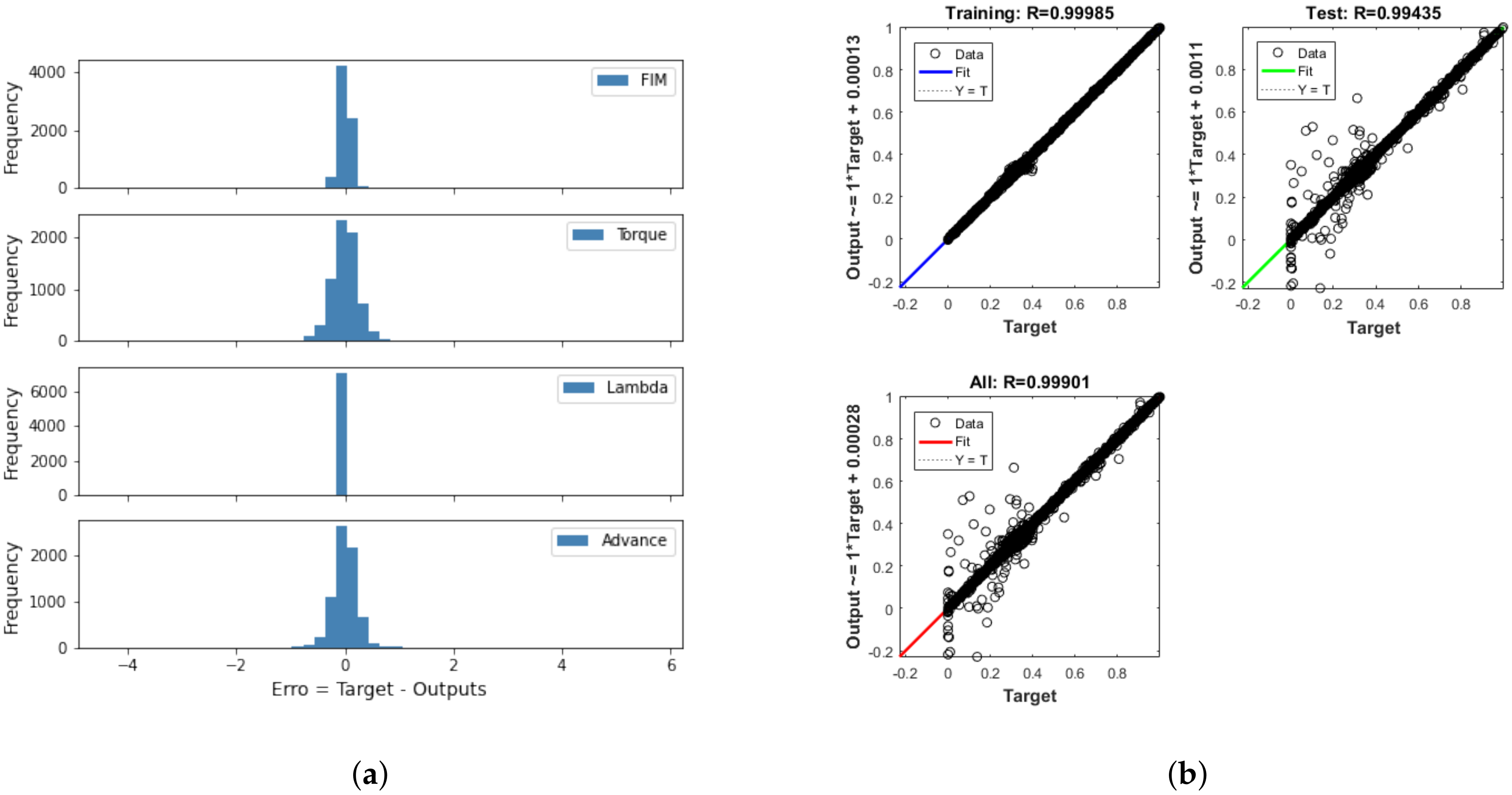
During the training phase using the Bayesian regularization backpropagation, as shown in Figure 10, the general regression was equal to 0.99901, which shows that the neural network also correlated the network input variables with the output variables very well. It is also observed, via the histogram of errors, that the vast majority of errors were close to 0, showing that the algorithm was effective at minimizing the performance index based on the adjustment of the ANN weights; that is, learning.
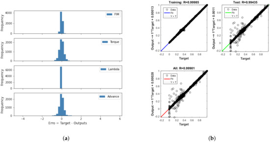
Figure 10.
(a) Histogram of errors and (b) regression during ANN training using the Bayesian regularization backpropagation.
Then, using the best configuration found from each learning algorithm, we created four ANNs. Two ANNs were created with the Levenberg–Marquardt backpropagation using 43% and 65% of data, and two ANNs were created with the Bayesian regularization backpropagation using 43% and 65 % of data. Those ANNs were used to simulate the output parameters of total acquisition points obtained in the bench test to evaluate the capacity for predicting the points that were not used for ANN training. The results precision are summarized in Table 6 and Table 7.
Table 6.
Precision of ANN trained with 43% of points.
Table 7.
Precision of ANN trained with 65% of points.
These results show that, by using 43% of data, the percentage of points that were within the acceptance criteria for the fuel injection mass, applied ignition advance, lambda, and torque, by training the ANN with the algorithm Levenberg–Marquardt backpropagation, were 76.73%, 64.80%, 95.80%, and 80.66%, respectively. However, with the same amount of data, the percentage of points was 94.47%, 84.75%, 94.05%, and 96.49% when training the ANN with the Bayesian regularization backpropagation algorithm. Moreover, by using 65% of data, the percentage raised for 90.10%, 81.30%, 97.62%, and 93.07% when training the ANN with the Levenberg–Marquardt backpropagation algorithm, and for 99.31%, 96.17%, 97.94%, and 99.41% when training the ANN with the algorithm Bayesian regularization backpropagation.
These results show that even using only 43% of data, the SI Engine can be effectively modeled with high accuracy by training the ANN with the Bayesian regularization backpropagation. Moreover, the Figure A2 shows the distribution of points where the fuel injection mass prediction error was higher than 3% when we simulated all Engine fields using the ANN model created with 65% of data. It is possible to confirm that simulation error was not concentrated in the region where data were not used to train the ANN, which gives them confidence that good modeling was achieved. Furthermore, high errors were observed at low engine speed, likely because of the high instability at this operation point.
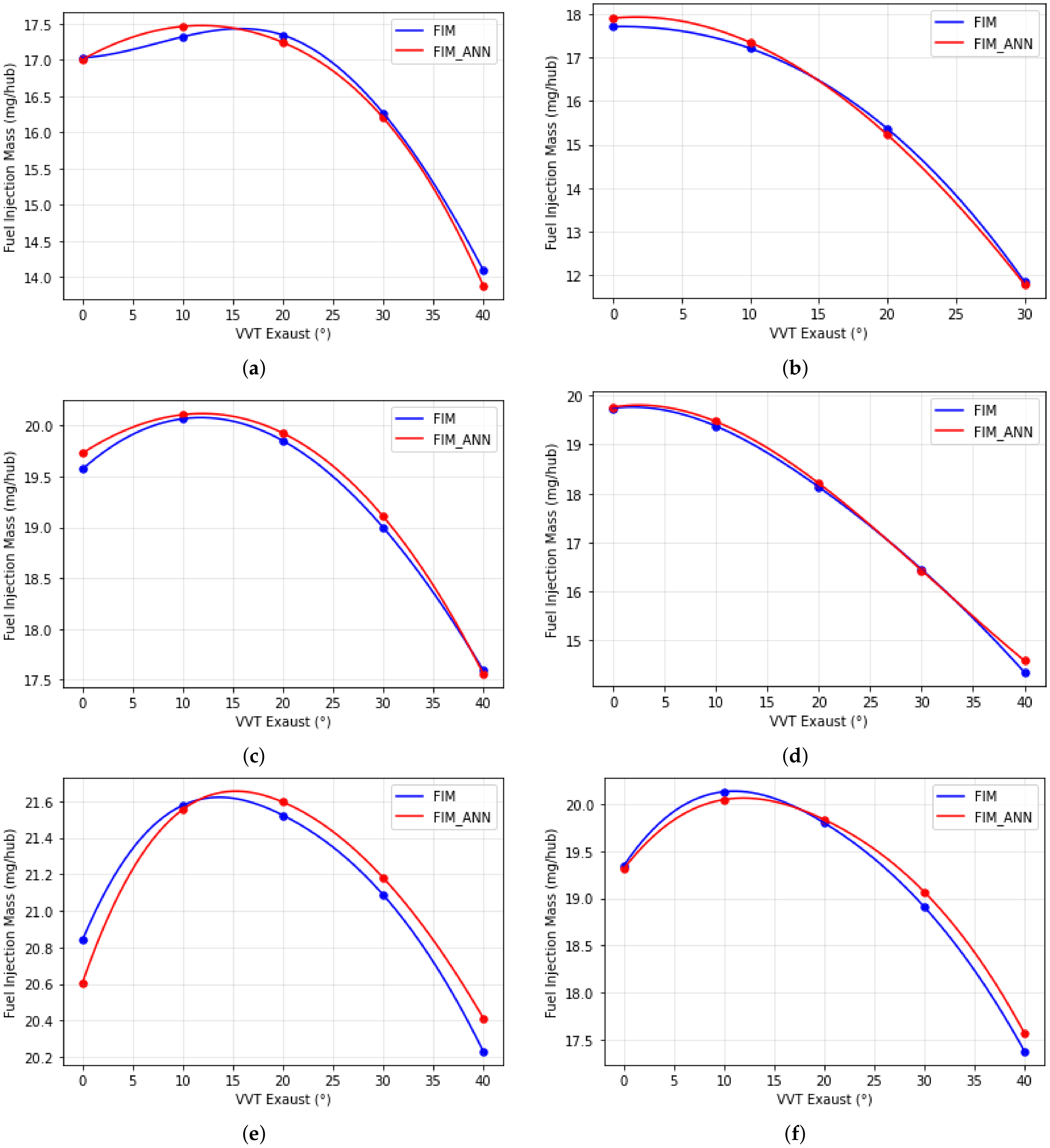
To make a more profound investigation of the results, some results were plotted with ANN generated by Bayesian Regularization backpropagation with 65% of data as input to check the coherence of modeling and the physical behavior. Figure 11 shows the acquired data versus ANN simulation of VVT’s parabolic fuel injection in the function of the VVT Exhaust at engine speed and VVT Intake, where the data were not used to create the ANN model in 540 mbar. It is possible to confirm that the learning profile is according the physical behavior.

Figure 11.
Fuel Injection Mass vs. VVT Exaust in 540 mbar and (a) Engine Speed = 1000 rpm/VVT_Intake = 10, (b) Engine Speed = 1000 rpm/VVT_Intake = 30, (c) Engine Speed = 3100 rpm/VVT_Intake = 20, (d) Engine Speed = 3100 rpm/VVT_Intake = 40, (e) Engine Speed = 5800 rpm/VVT_Intake = 10, (f) Engine Speed = 5800 rpm/VVT_Intake = 30.
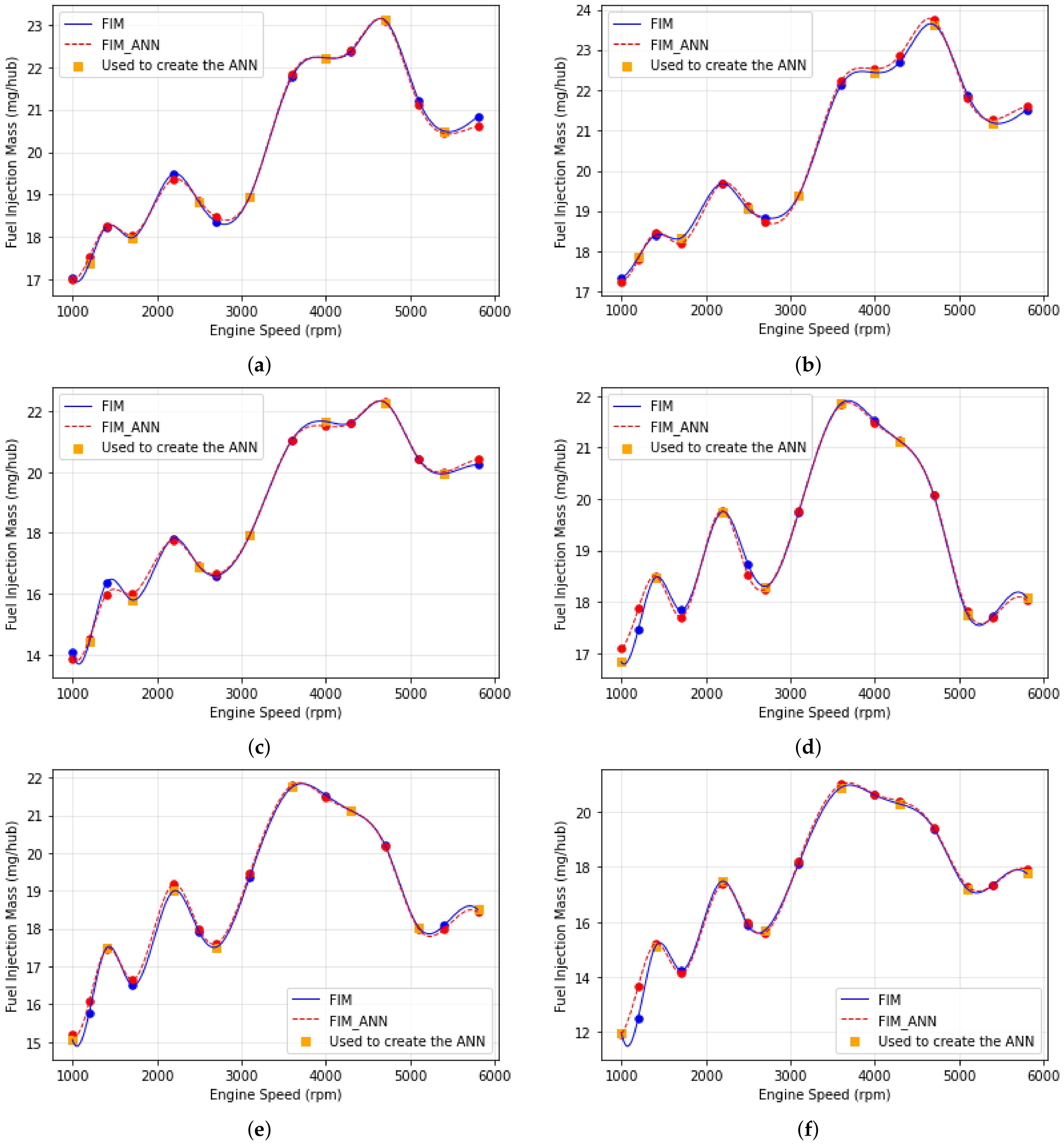
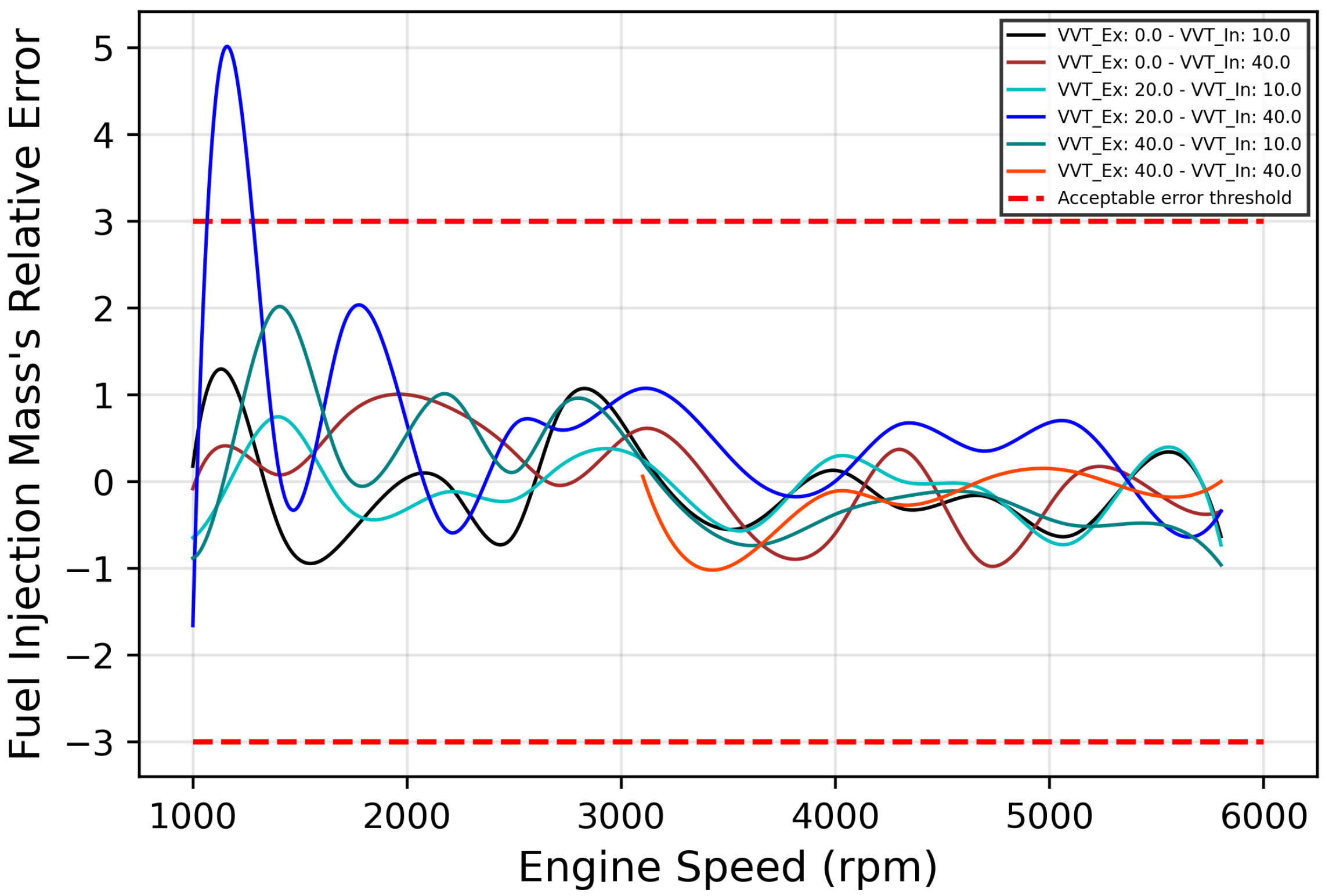
Moreover, to check the capacity of the ANN for predicting the points that were not used to train the model, Figure 12 shows the acquired data versus ANN simulation versus the data used to create ANN in function of engine speed at 540 mbar. It is possible to confirm that the learning profile is according to the physical behavior, and the ANN can correctly predict the points that were not used to train. The relative errors between acquired data and ANN simulation are shown in Figure 13.
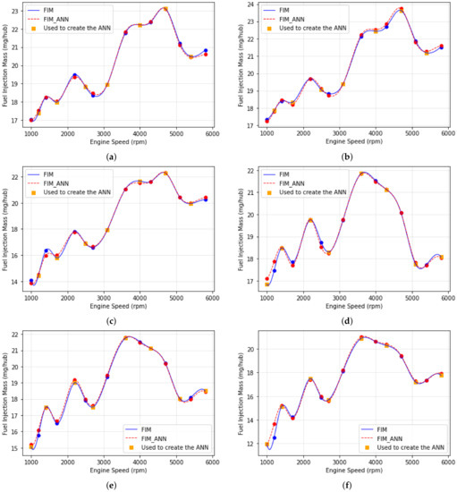
Figure 12.
Fuel Injection Mass vs. Engine Speed in 540 mbar and (a) VVT_Exaust = 0/VVT_Intake = 10, (b) VVT_Exaust = 20/VVT_Intake = 10, (c) VVT_Exaust = 40/VVT_Intake = 10, (d) VVT_Exaust = 0/VVT_Intake = 40, (e) VVT_Exaust = 10/VVT_Intake = 40, (f) VVT_Exaust = 20/VVT_Intake = 40.

Figure 13.
Fuel Injection Mass’ Relative Error Graph.
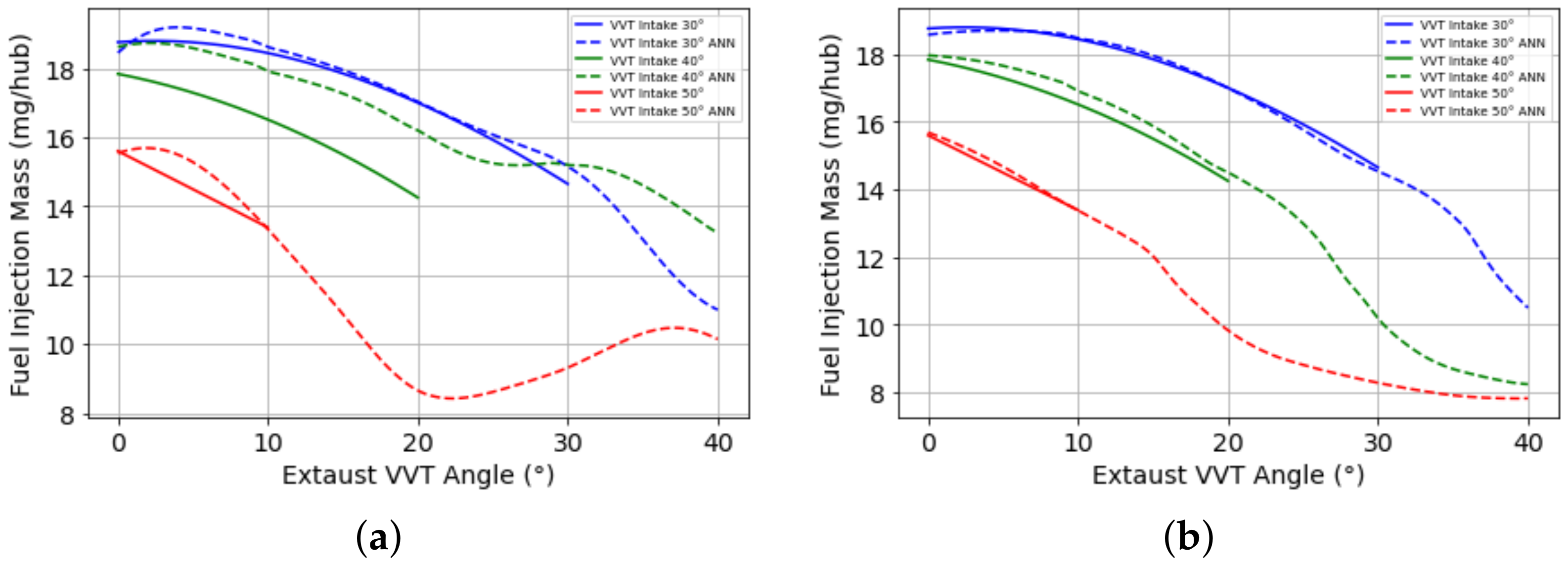
To check the capacity of ANN prediction, the physical behavior and the extrapolation capacity was simulated the fuel injection as a function of exhaust VVT angle in steps of 1°. It was possible to check, as shown in Figure 14, that all points in the range of measured data respect the parabolic profile, giving us confidence that accurate modeling was performed. The extrapolation worked well: only 10° higher than the maximum measured exhaust VVT angle. Values higher than that diverged from the parabolic profile. It is impossible to confirm if the model correctly predicted the overlap effect in intake mass flow or if it was a measurement error because the engine presented high combustion instability at these points. It was not possible to measure it.
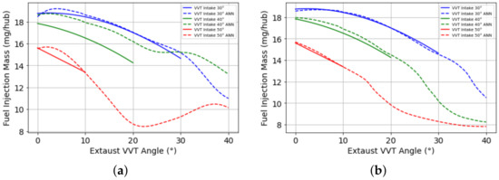
Figure 14.
ANN’s extrapolation capacity of the fuel injection as function of exhaust VVT angle in steps of 1° (a) using Levenberg–Marquardt backpropagation and (b) using Bayesian regularization backpropagation.
6. Conclusions
Spark Ignition Engine is a complex thermal machine. The virtualization might help us to better figure out its behavior and enable development of control algorithms and management systems in terms of accuracy and precision. The artificial neural network is a powerful tool that models the physical system.
The present work had the objective of proposing a versatile method for auto-modeling an Engine Black-Box model based on a feedforward Artificial Neural Network for tuning development purposes. We evaluated and compared the performance in terms of accuracy and computational cost; two neural network training functions: Levenberg–Marquardt backpropagation and Bayesian regularization backpropagation, made available by the Matlab Neural Network Toolbox, were investigated. The genetic algorithm was implemented for optimization purposes to find an ANN architecture that provides a virtual model of the engine with an acceptable estimation rate of the variables to be modeled.
To assess our proposed methodology, the following parameters were used as input for the ANN model: Engine Speed, Intake Manifold Pressure, Intake VVT Angle, and Exhaust VVT Angle. The model’s outputs were: fuel injection mass, lambda, torque, and applied ignition advance. The results obtained show that our method has excellent potential for the development of virtual models of internal combustion engines since, using only 43% of the data from the entire engine field to train the ANN, the best model found when simulating the entire field of the engine, our model met 94.47%, 84.75%, 94.05%, and 96.49% of the acceptance criteria for the fuel injection mass, applied ignition advance, lambda, and torque, respectively, by training the ANN with Bayesian regularization backpropagation. Experimental outcomes were presented in this paper, demonstrating the efficiency of our approach and showing that the genetic algorithm, in an acceptable time, can effectively optimize the ANN engine model. The ANN trained using the Bayesian regularization backpropagation is more accurate and reliable than the ones trained using the Levenberg–Marquardt backpropagation.
For future work, one can first implement other selection methods within GA to assess the method that performs best. Different types of meta-heuristic algorithms, such as PSO and DE, can also be implemented to optimize the neural network architecture to determine the algorithm that presents the best result and compare their respective computational costs.
Author Contributions
Literature search, H.G.T.; methodology, H.G.T. and S.A.B.J.; investigation, H.G.T. and S.A.B.J.; simulations, H.G.T.; visualization, H.G.T.; data analysis, H.G.T. and S.A.B.J.; data interpretation H.G.T. and S.A.B.J.; writing—original draft preparation, H.G.T., S.A.B.J. and M.M.D.S.; writing-review and editing, H.G.T., S.A.B.J. and M.M.D.S.; study design, S.A.B.J., R.B. and M.M.D.S.; data collection, S.A.B.J. and R.B.; supervision R.B. and M.M.D.S.; project administration, R.B. All authors have read and agreed to the published version of the manuscript.
Funding
This work was supported by Renault Brazil and Fundação Araucária.
Institutional Review Board Statement
Not applicable.
Informed Consent Statement
Not applicable.
Data Availability Statement
Not applicable.
Acknowledgments
We acknowledge the support from Renault Brazil, Fundação Araucária and Universidade Tecnológica Federal do Paraná - Ponta Grossa through computational resource grants, expertise, technical support and financial support.
Conflicts of Interest
The authors declare no conflict of interest.
Abbreviations
The following abbreviations are used in this manuscript:
| AFR | Air–fuel ratio. |
| ANN | Artificial Neural Network. |
| CO | Carbon monoxide. |
| DE | Differential Evolution. |
| ECU | Engine Control Unit. |
| FIM | Fuel Injection Mass. |
| GA | Genetic Algorithm. |
| MAE | Mean Absolute Error. |
| MAPE | Mean Absolute Percent Error. |
| MLP | Multi-layer perceptrons. |
| MSE | Mean Square Error. |
| MVM | Mean Value Model. |
| NOx | Nitrogen oxide. |
| PSO | Particle Swarm Optimization. |
| RBF | Radial Basis Function. |
| SVM | Support vector machine. |
| QRNG | Quasi-random number generator. |
| RMSE | Root Mean Square Error. |
| VVT | Variable Valve Timing. |
Appendix A
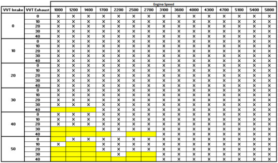
Figure A1.
Acquisition points.
Figure A1.
Acquisition points.
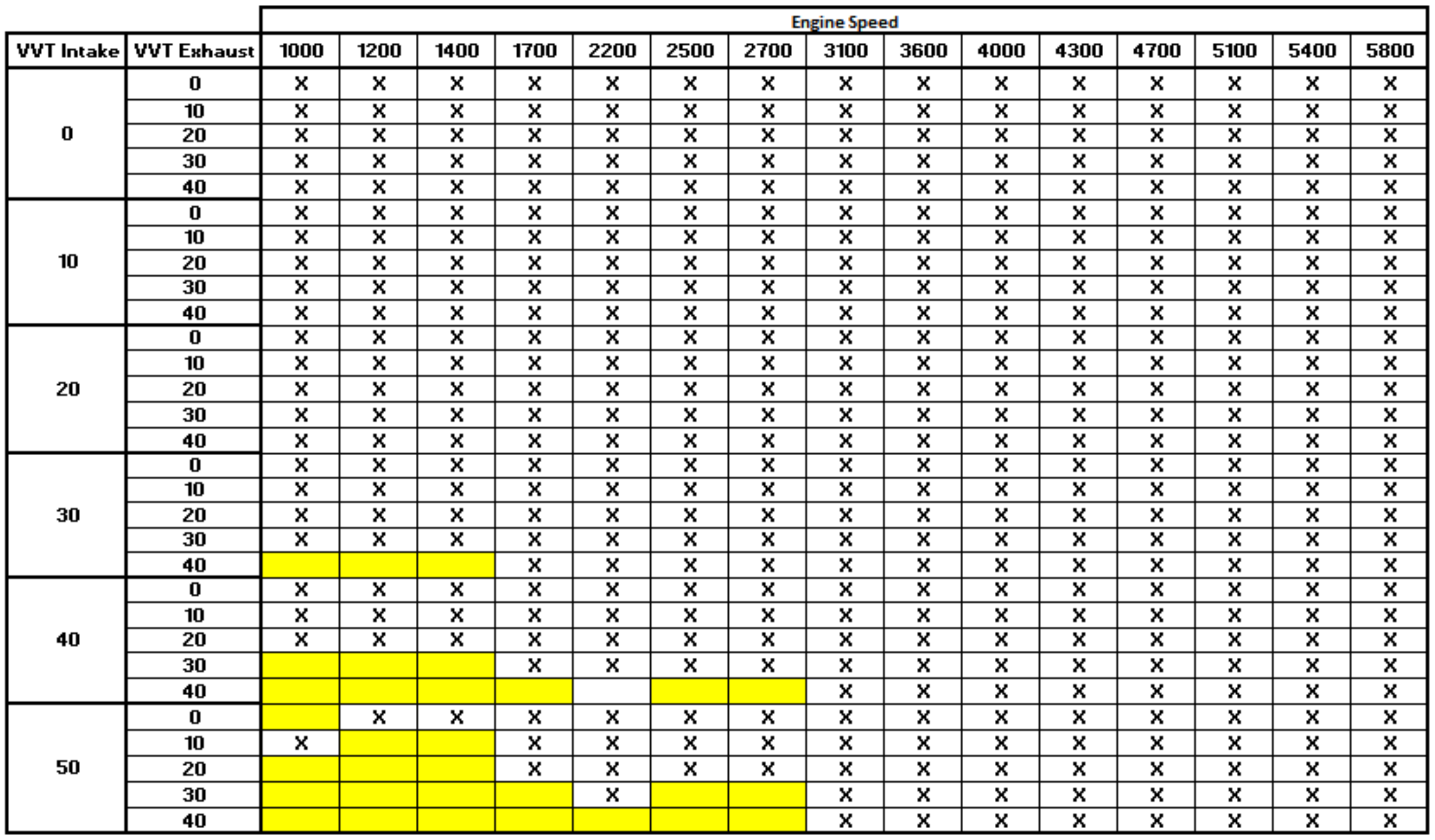
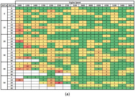
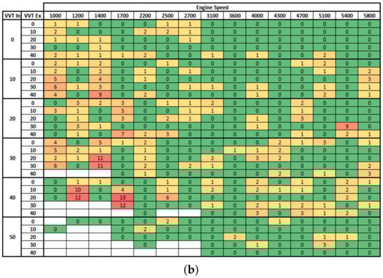
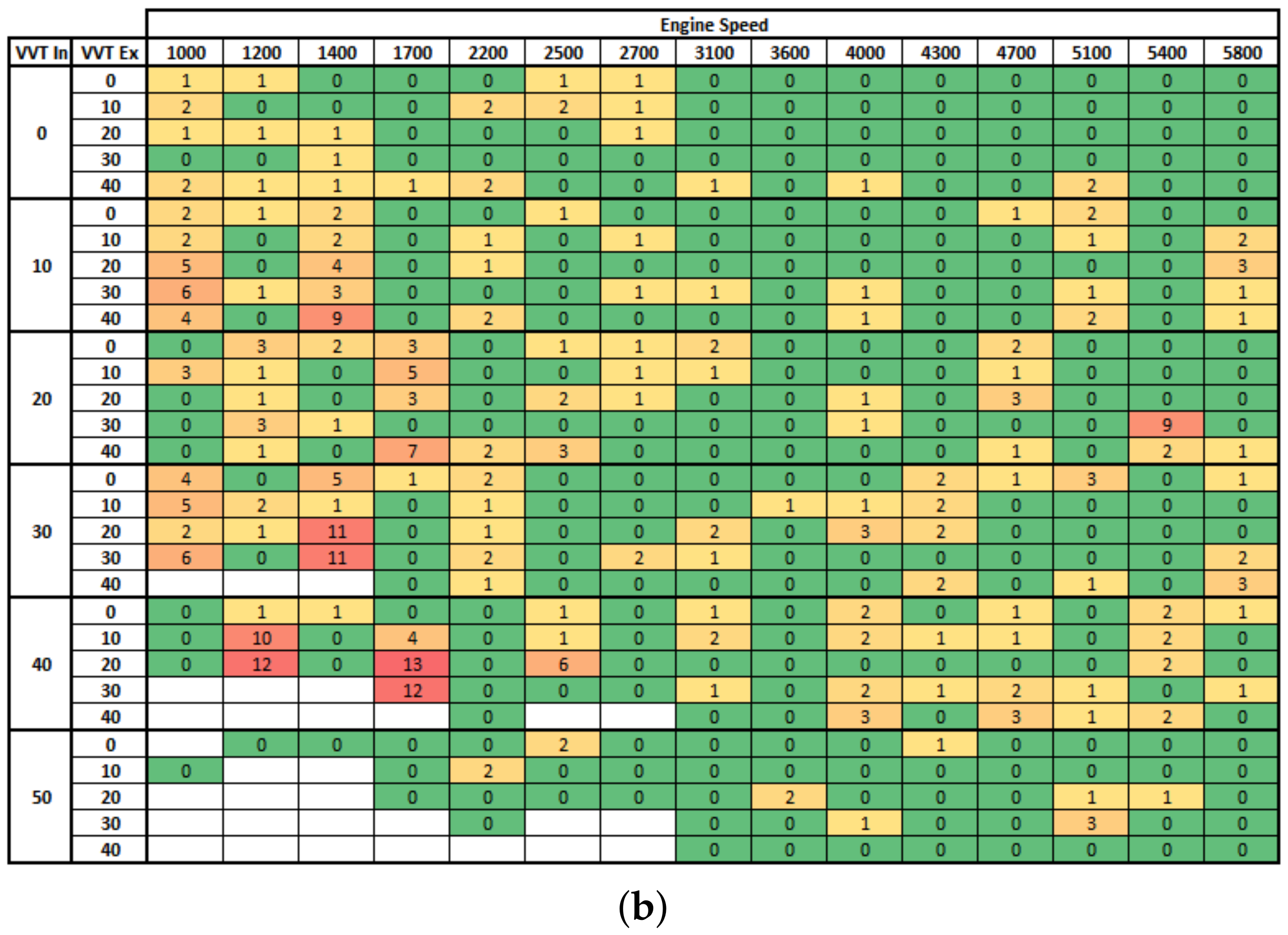
Figure A2.
Distribution of points where the fuel injection mass prediction erro was higher than 3% (a) Levenberg–Marquardt backpropagation, (b) Bayesian regularization backpropagation.
Figure A2.
Distribution of points where the fuel injection mass prediction erro was higher than 3% (a) Levenberg–Marquardt backpropagation, (b) Bayesian regularization backpropagation.
References
- Wang, S.; Yu, D.; Gomm, J.; Page, G.; Douglas, S. Adaptive neural network model based predictive control for air–fuel ratio of SI engines. Eng. Appl. Artif. Intell. 2006, 19, 189–200. [Google Scholar] [CrossRef]
- Roepke, K. Design of Experiments for Engine Calibration. J. Soc. Instrum. Control. Eng. 2014, 53, 322–327. [Google Scholar]
- Turkson, R.F.; Yan, F.; Ali, M.K.A.; Hu, J. Artificial neural network applications in the calibration of spark-ignition engines: An overview. Eng. Sci. Technol. Int. J. 2016, 19, 1346–1359. [Google Scholar] [CrossRef]
- Mohamed, Z.E. Using the artificial neural networks for prediction and validating solar radiation. J. Egypt. Math. Soc. 2019, 27, 47. [Google Scholar] [CrossRef]
- Zhao, J.; Xu, M.; Li, M.; Wang, B.; Liu, S. Design and optimization of an Atkinson cycle engine with the Artificial Neural Network Method. Appl. Energy 2012, 92, 492–502. [Google Scholar] [CrossRef]
- Zhou, Q.; Gullitti, A.; Xiao, J.; Huang, Y. Neural Network–Based Modeling and Optimization for Effective Vehicle Emission Testing and Engine Calibration. Chem. Eng. Commun. 2008, 195, 706–720. [Google Scholar] [CrossRef]
- Benardos, P.; Vosniakos, G.C. Optimizing feedforward artificial neural network architecture. Eng. Appl. Artif. Intell. 2007, 20, 365–382. [Google Scholar] [CrossRef]
- Carvalho, A.R.; Ramos, F.M.; Chaves, A.A. Metaheuristics for the feedforward artificial neural network (ANN) architecture optimization problem. Neural Comput. Appl. 2011, 20, 1273–1284. [Google Scholar] [CrossRef]
- ul Islam, B.; Baharudin, Z.; Raza, M.Q.; Nallagownden, P. Optimization of neural network architecture using genetic algorithm for load forecasting. In Proceedings of the 2014 5th International Conference on Intelligent and Advanced Systems (ICIAS), Kuala Lumpur, Malaysia, 3–5 June 2014; IEEE: Piscataway, NJ, USA, 2014; pp. 1–6. [Google Scholar]
- Du Ke-Lin, S.M. Search and Optimization by Metaheuristics, Techniques and Algorithms Inspired by Nature; Springer: Berlin/Heidelberg, Germany, 2016; pp. 1–10. [Google Scholar]
- Ezugwu, A.E.; Adeleke, O.J.; Akinyelu, A.A.; Viriri, S. A conceptual comparison of several metaheuristic algorithms on continuous optimisation problems. Neural Comput. Appl. 2020, 32, 6207–6251. [Google Scholar] [CrossRef]
- Holland, J.H. Genetic algorithms. Sci. Am. 1992, 267, 66–73. [Google Scholar] [CrossRef]
- Wang, K.P.; Huang, L.; Zhou, C.G.; Pang, W. Particle swarm optimization for traveling salesman problem. In Proceedings of the 2003 International Conference on Machine Learning and Cybernetics (IEEE cat. no. 03ex693), Xi’an, China, 5 November 2003; IEEE: Piscataway, NJ, USA, 2003; Volume 3, pp. 1583–1585. [Google Scholar]
- Dorigo, M.; Birattari, M.; Stutzle, T. Ant colony optimization. IEEE Comput. Intell. Mag. 2006, 1, 28–39. [Google Scholar] [CrossRef]
- Cheng, M.Y.; Prayogo, D. Symbiotic organisms search: A new metaheuristic optimization algorithm. Comput. Struct. 2014, 139, 98–112. [Google Scholar] [CrossRef]
- Yang, X.S.; Deb, S. Cuckoo search via Lévy flights. In Proceedings of the 2009 World Congress on nature & Biologically Inspired Computing (NaBIC), Coimbatore, India, 9–11 December 2009; IEEE: Piscataway, NJ, USA, 2009; pp. 210–214. [Google Scholar]
- Fister, I.; Fister Jr, I.; Yang, X.S.; Brest, J. A comprehensive review of firefly algorithms. Swarm Evol. Comput. 2013, 13, 34–46. [Google Scholar] [CrossRef]
- Karaboga, D.; Basturk, B. A powerful and efficient algorithm for numerical function optimization: Artificial bee colony (ABC) algorithm. J. Glob. Optim. 2007, 39, 459–471. [Google Scholar] [CrossRef]
- Yang, X.S. A new metaheuristic bat-inspired algorithm. In Nature Inspired Cooperative Strategies for Optimization (NICSO 2010); Springer: Berlin/Heidelberg, Germany, 2010; pp. 65–74. [Google Scholar]
- Ab Wahab, M.N.; Nefti-Meziani, S.; Atyabi, A. A comprehensive review of swarm optimization algorithms. PLoS ONE 2015, 10, e0122827. [Google Scholar] [CrossRef]
- Yang, X.S. Flower pollination algorithm for global optimization. In Proceedings of the International Conference on Unconventional Computing and Natural Computation, Orleans, France, 3–7 September 2012; Springer: Berlin/Heidelberg, Germany, 2012; pp. 240–249. [Google Scholar]
- Mehrabian, A.R.; Lucas, C. A novel numerical optimization algorithm inspired from weed colonization. Ecol. Inform. 2006, 1, 355–366. [Google Scholar] [CrossRef]
- Pham, D.T.; Castellani, M. The bees algorithm: Modelling foraging behaviour to solve continuous optimization problems. Proc. Inst. Mech. Eng. Part C J. Mech. Eng. Sci. 2009, 223, 2919–2938. [Google Scholar] [CrossRef]
- Ramadhas, A.; Jayaraj, S.; Muraleedharan, C. Theoretical modeling and experimental studies on biodiesel-fueled engine. Renew. Energy 2006, 31, 1813–1826. [Google Scholar] [CrossRef]
- Jung, D. Residual Generation Using Physically-Based Grey-Box Recurrent Neural Networks For Engine Fault Diagnosis. arXiv 2020, arXiv:2008.04644. [Google Scholar]
- Zanardo, G.; Stadlbauer, S.; Waschl, H.; del Re, L. Grey Box Control Oriented SCR Model. Technical Report, SAE Technical Paper. 2013. Available online: https://www.sae.org/publications/technical-papers/content/2013-24-0159/ (accessed on 15 July 2022).
- Nickmehr, N. System Identification of an Engine-Load Setup Using Grey-Box Model. Ph.D. Thesis, Linköping University, Linköping, Sweden, 2014. [Google Scholar]
- Shamekhi, A.M.; Shamekhi, A.H. A new approach in improvement of mean value models for spark ignition engines using neural networks. Expert Syst. Appl. 2015, 42, 5192–5218. [Google Scholar] [CrossRef]
- Hendricks, E. The analysis of mean value engine models. SAE Trans. 1989, 98, 972–985. [Google Scholar]
- Nazoktabar, M.; Jazayeri, S.A.; Arshtabar, K.; Ganji, D.D. Developing a multi-zone model for a HCCI engine to obtain optimal conditions using genetic algorithm. Energy Convers. Manag. 2018, 157, 49–58. [Google Scholar] [CrossRef]
- Isermann, R. Engine Modeling and Control; Springer: Berlin/Heidelberg, Germany, 2014; Volume 1017. [Google Scholar]
- De Nicolao, G.; Scattolini, R.; Siviero, C. Modelling the volumetric efficiency of IC engines: Parametric, non-parametric and neural techniques. Control Eng. Pract. 1996, 4, 1405–1415. [Google Scholar] [CrossRef]
- De Nola, F.; Giardiello, G.; Gimelli, A.; Molteni, A.; Muccillo, M.; Picariello, R. Volumetric efficiency estimation based on neural networks to reduce the experimental effort in engine base calibration. Fuel 2019, 244, 31–39. [Google Scholar] [CrossRef]
- Najafi, G.; Ghobadian, B.; Moosavian, A.; Yusaf, T.; Mamat, R.; Kettner, M.; Azmi, W. SVM and ANFIS for prediction of performance and exhaust emissions of a SI engine with gasoline–ethanol blended fuels. Appl. Therm. Eng. 2016, 95, 186–203. [Google Scholar] [CrossRef]
- Hao, D.; Mehra, R.K.; Luo, S.; Nie, Z.; Ren, X.; Fanhua, M. Experimental study of hydrogen enriched compressed natural gas (HCNG) engine and application of support vector machine (SVM) on prediction of engine performance at specific condition. Int. J. Hydrog. Energy 2020, 45, 5309–5325. [Google Scholar] [CrossRef]
- Norouzi, A.; Aliramezani, M.; Koch, C.R. A correlation-based model order reduction approach for a diesel engine NOx and brake mean effective pressure dynamic model using machine learning. Int. J. Engine Res. 2020, 1468087420936949. [Google Scholar] [CrossRef]
- He, Y.; Rutland, C. Application of artificial neural networks in engine modelling. Int. J. Engine Res. 2004, 5, 281–296. [Google Scholar] [CrossRef]
- Niu, X.; Yang, C.; Wang, H.; Wang, Y. Investigation of ANN and SVM based on limited samples for performance and emissions prediction of a CRDI-assisted marine diesel engine. Appl. Therm. Eng. 2017, 111, 1353–1364. [Google Scholar] [CrossRef]
- Subana, S.; Samarasinghe, S. Artificial Neural Network Modelling; Springer: Cham, Switzerland, 2016. [Google Scholar]
- Maaranen, H.; Miettinen, K.; Mäkelä, M.M. Quasi-random initial population for genetic algorithms. Comput. Math. Appl. 2004, 47, 1885–1895. [Google Scholar] [CrossRef]
- Siqueira, H.; Boccato, L.; Luna, I.; Attux, R.; Lyra, C. Performance analysis of unorganized machines in streamflow forecasting of Brazilian plants. Appl. Soft Comput. 2018, 68, 494–506. [Google Scholar] [CrossRef]
- Umar, A.; Sulaiman, I.; Mamat, M.; Waziri, M.; Zamri, N. On damping parameters of Levenberg-Marquardt algorithm for nonlinear least square problems. J. Phys. Conf. Ser. IOP Publ. 2021, 1734, 012018. [Google Scholar] [CrossRef]
- Gavin, H.P. The Levenberg-Marquardt Algorithm for Nonlinear Least Squares Curve-Fitting Problems; Department of Civil and Environmental Engineering, Duke University: Durham, NC, USA, 2019; pp. 1–19. Available online: http://people.duke.edu/~{}hpgavin/ce281/lm.pdf (accessed on 15 July 2022).
- Hagan, M.T.; Demuth, H.B.; Beale, M. Neural Network Design; PWS Publishing Co.: Boston, MA, USA, 1997. [Google Scholar]
- Anand, S.; Afreen, N.; Yazdani, S. A novel and efficient selection method in genetic algorithm. Int. J. Comput. Appl. 2015, 129, 7–12. [Google Scholar] [CrossRef]
- Burden, F.; Winkler, D. Bayesian regularization of neural networks. Artif. Neural Netw. 2008, 23–42. [Google Scholar]
- Katoch, S.; Chauhan, S.S.; Kumar, V. A review on genetic algorithm: Past, present, and future. Multimed. Tools Appl. 2021, 80, 8091–8126. [Google Scholar] [CrossRef]


Publisher’s Note: MDPI stays neutral with regard to jurisdictional claims in published maps and institutional affiliations. |
© 2022 by the authors. Licensee MDPI, Basel, Switzerland. This article is an open access article distributed under the terms and conditions of the Creative Commons Attribution (CC BY) license (https://creativecommons.org/licenses/by/4.0/).