
Numerical Analysis of Two-Stage Turbine System for Multicylinder Engine under Pulse Flow Conditions with High Pressure-Ratio Turbine Rotor


Abstract
:1. Introduction
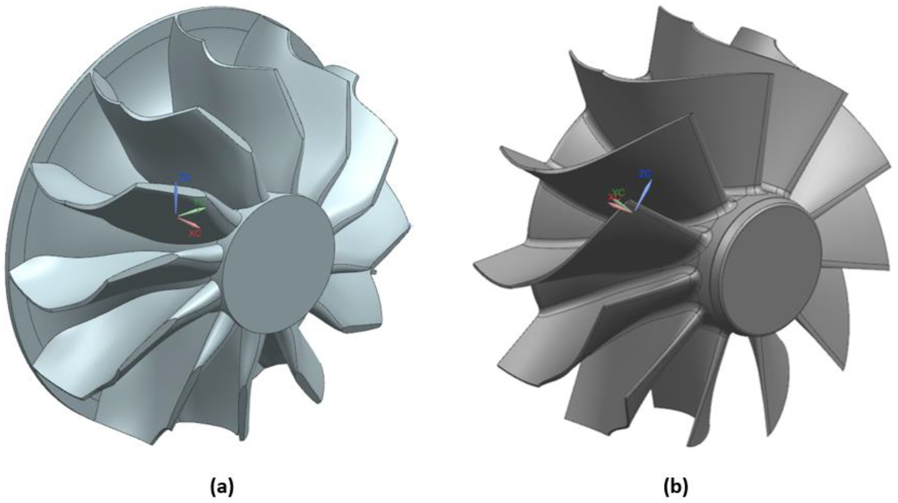
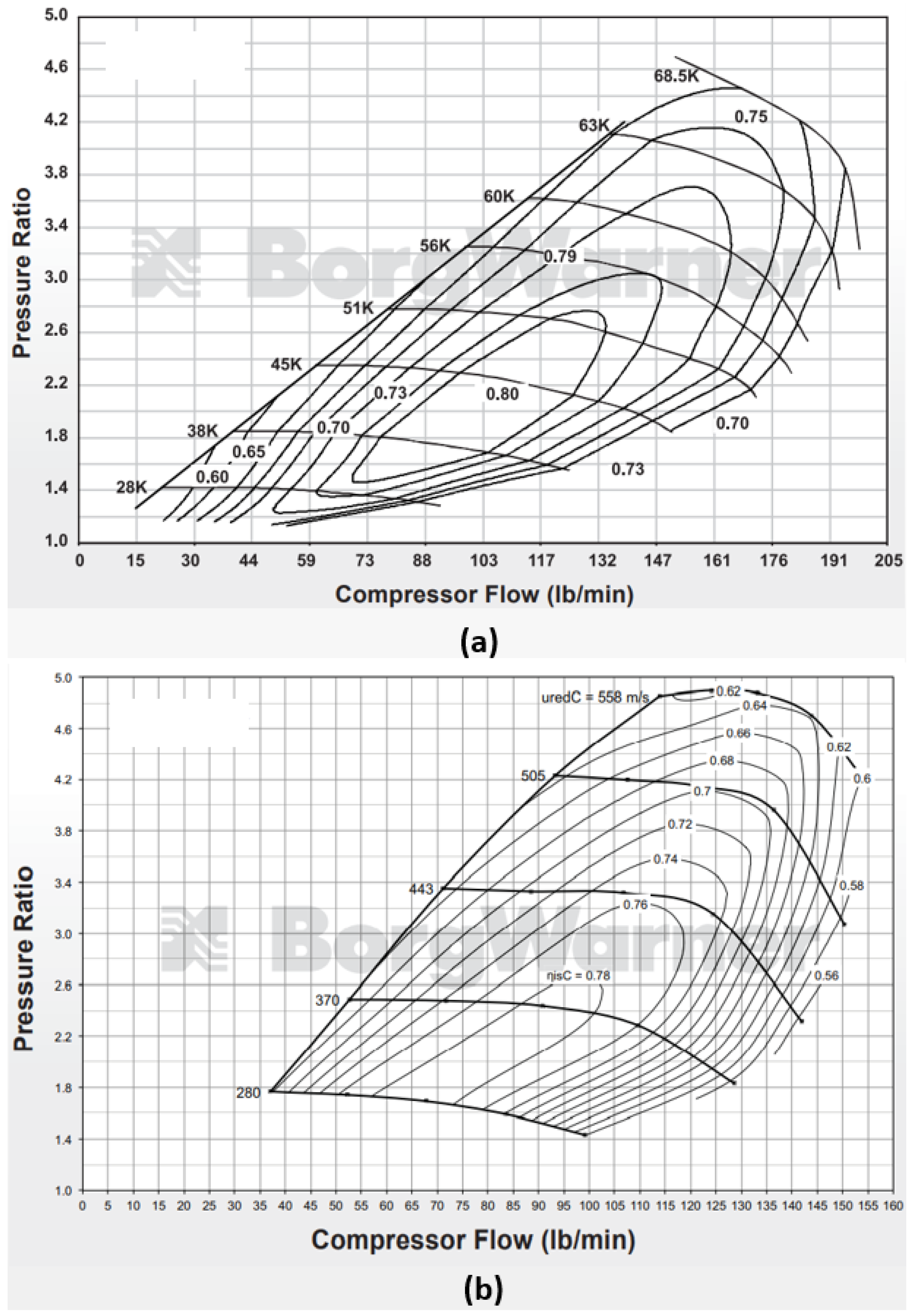
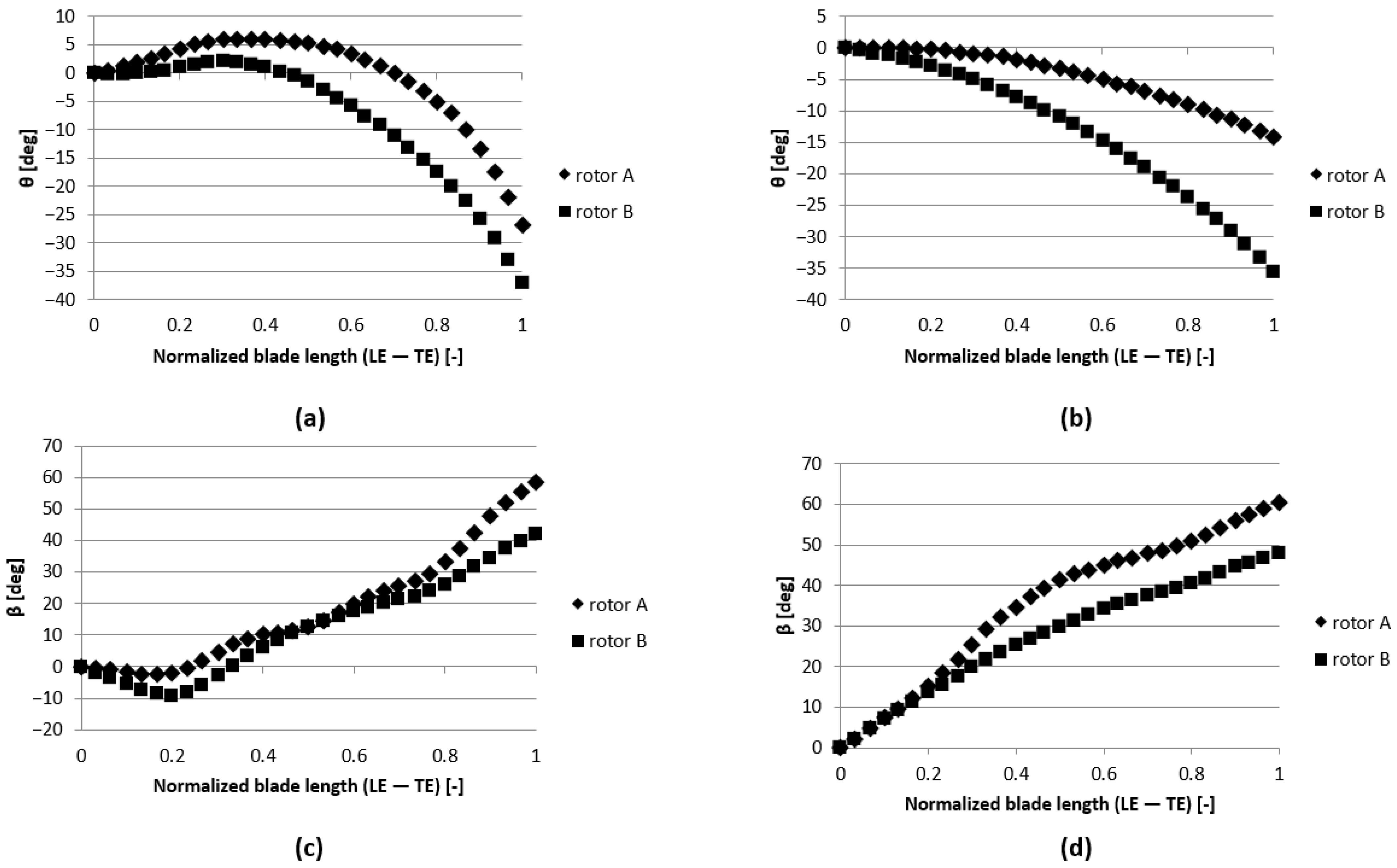
2. Rotor A and Rotor B
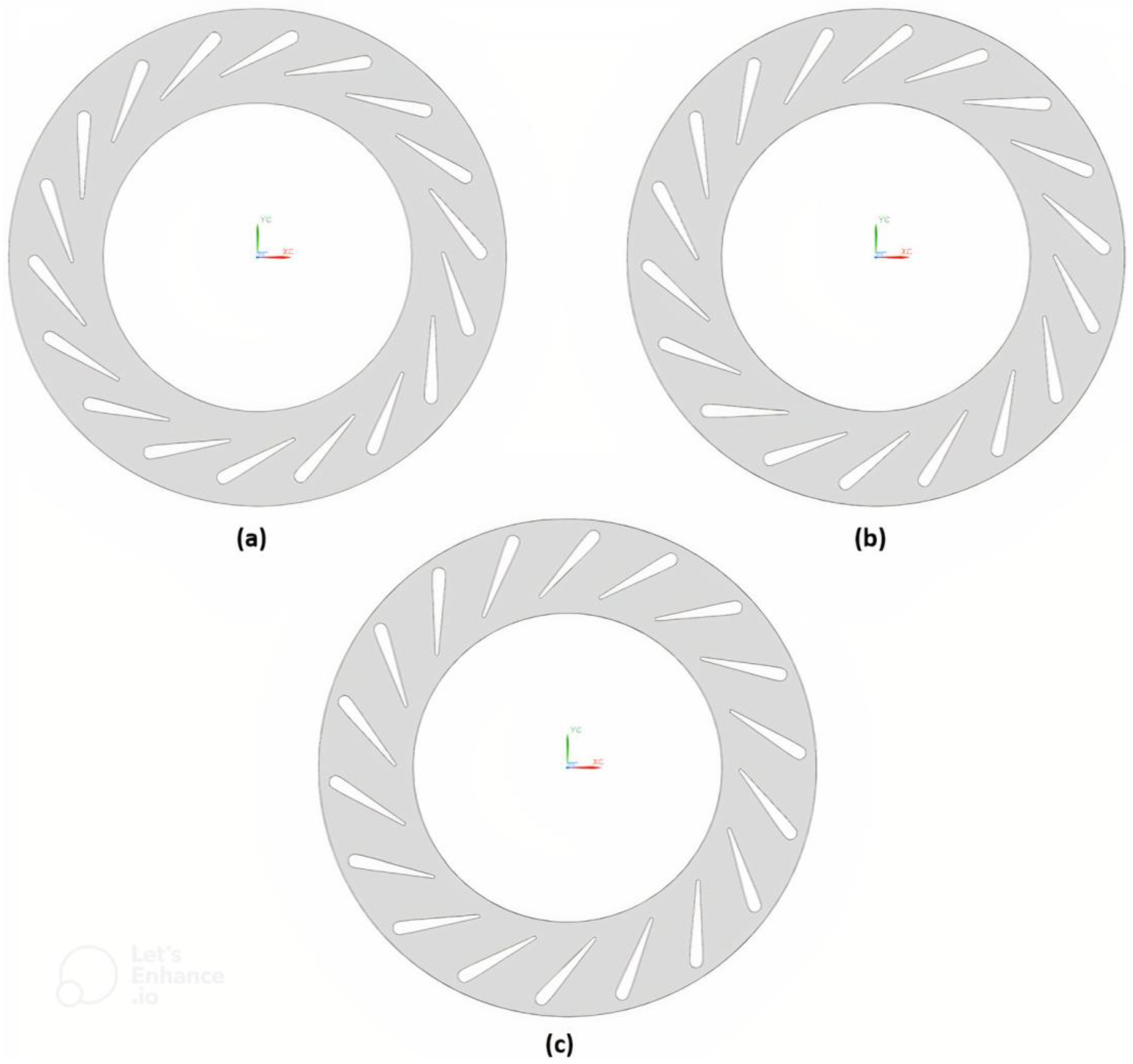
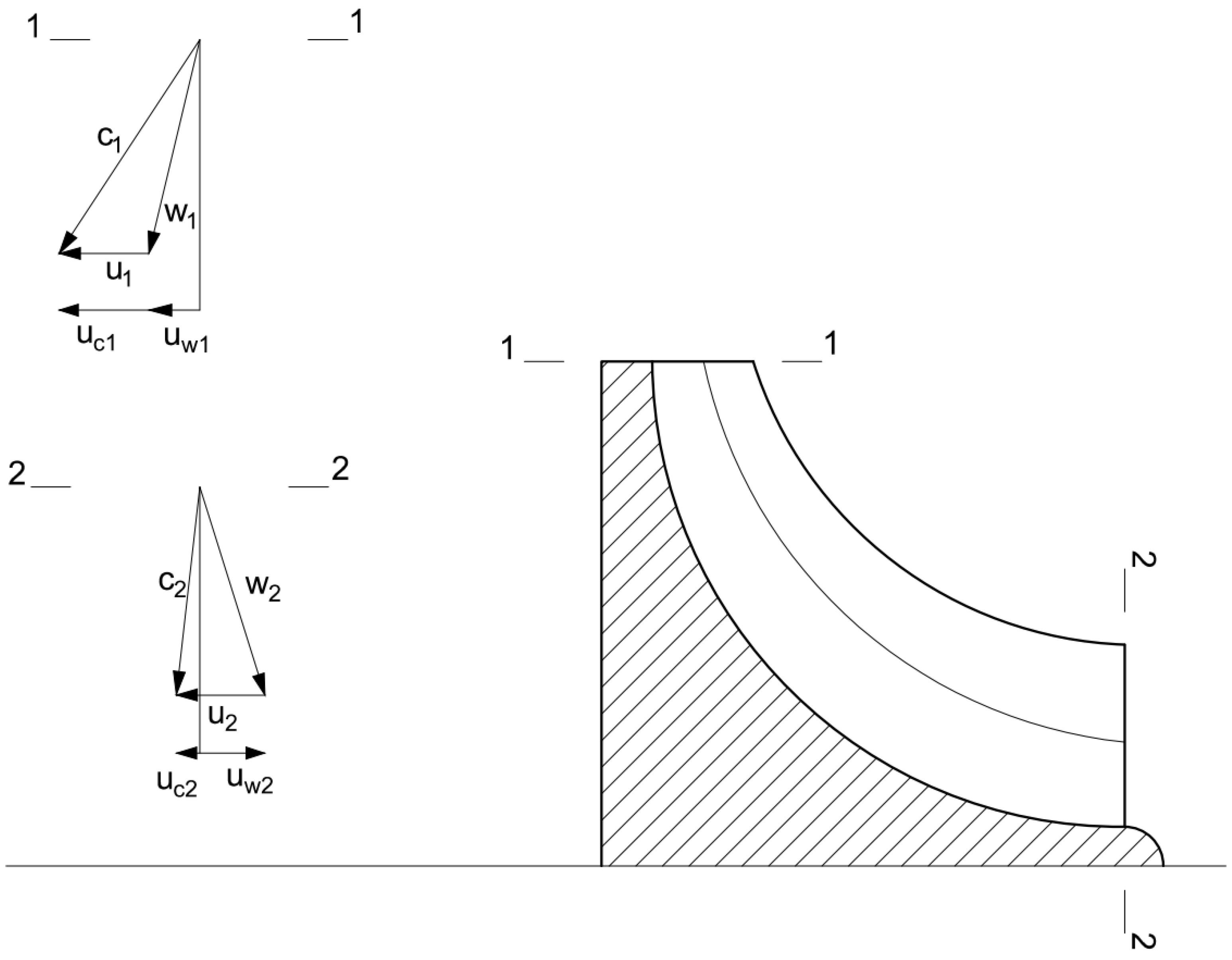
3. Radial Inflow Turbine
4. Numerical Domain
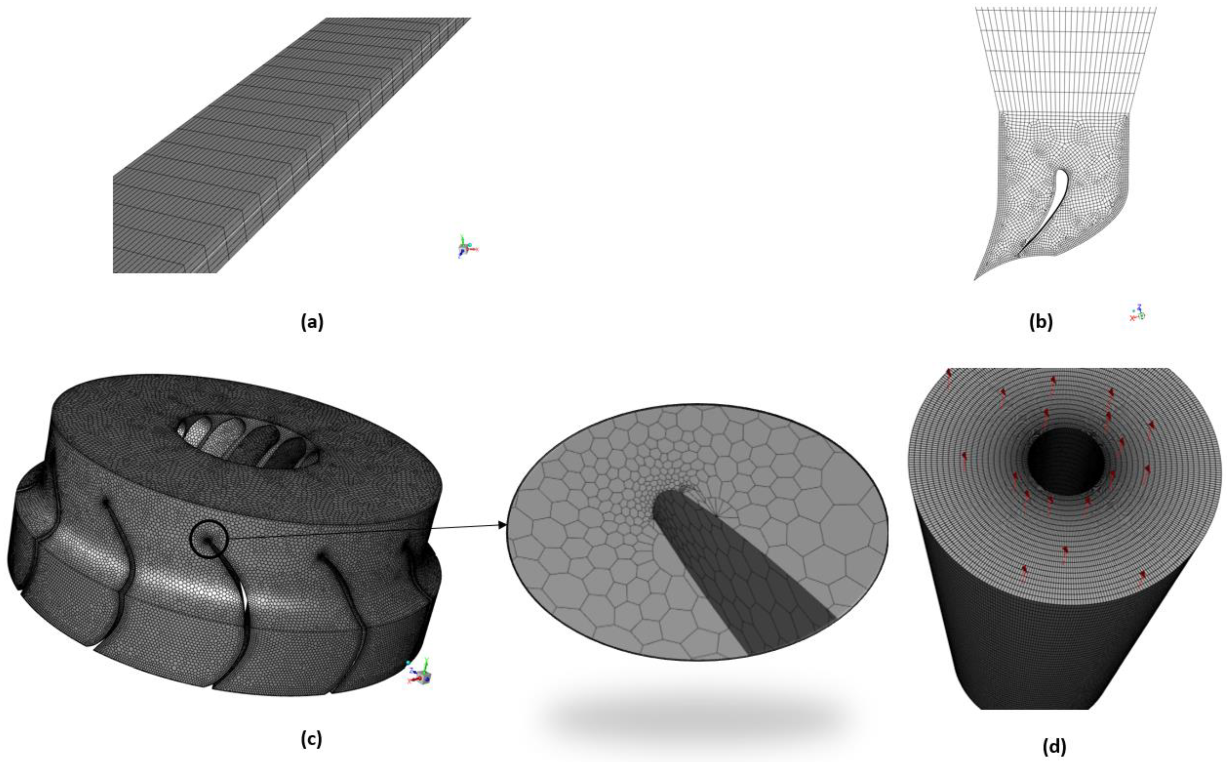
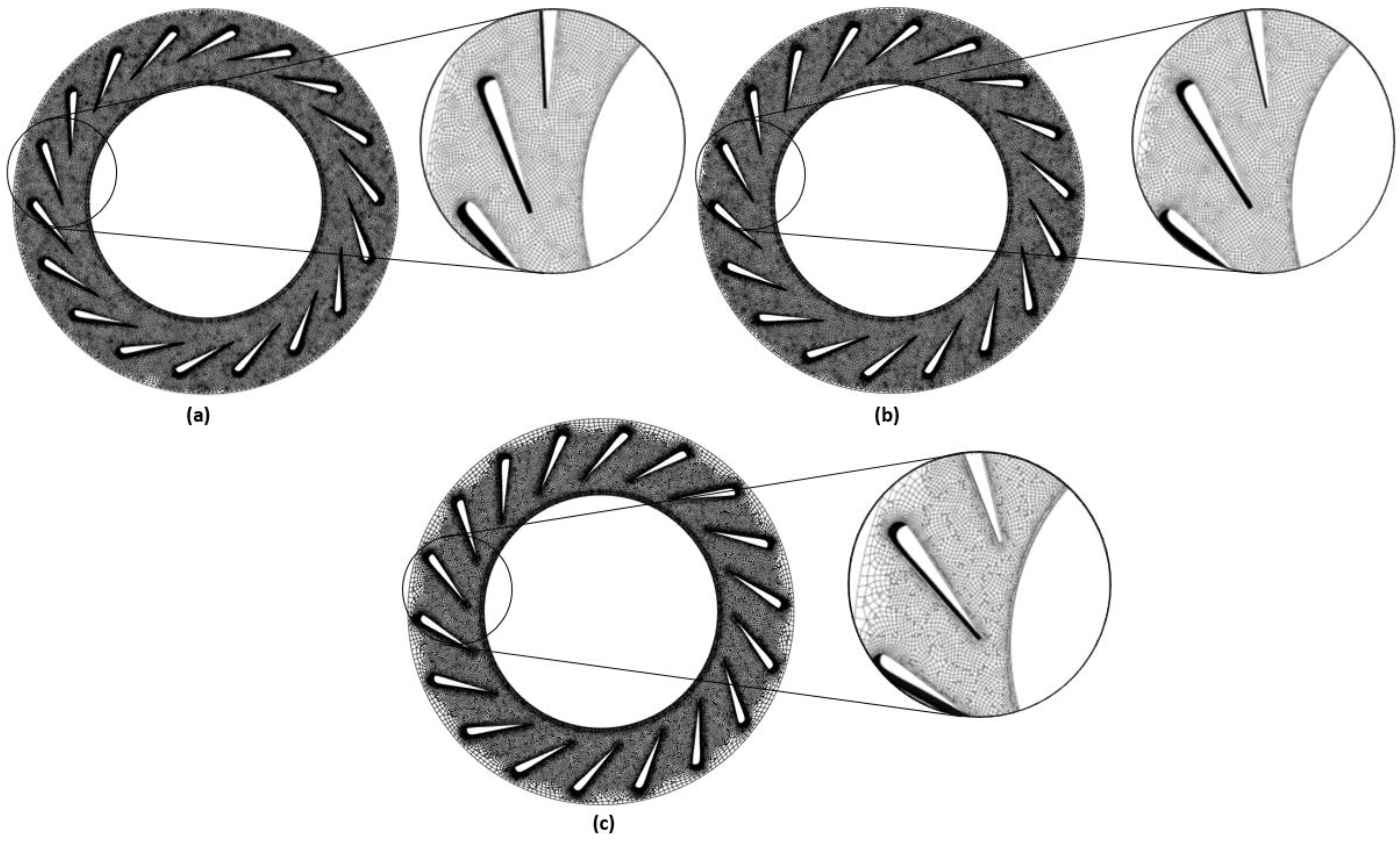
4.1. Numerical Mesh
4.2. Simulation Setup
4.3. Boundary Conditions
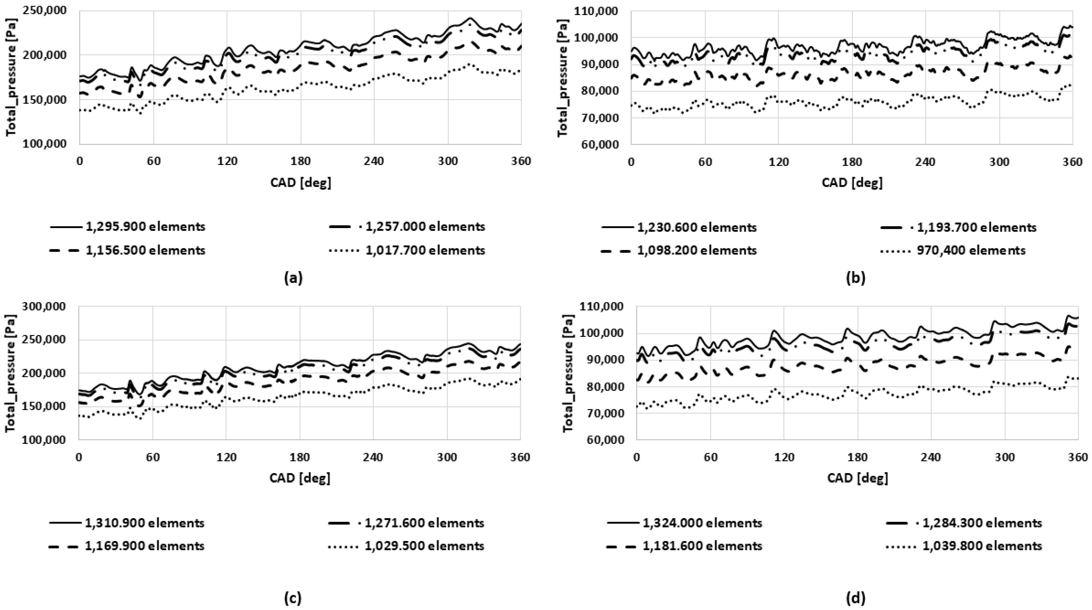
4.4. Mesh Validation
4.5. Model Validation
5. Results and Discussion
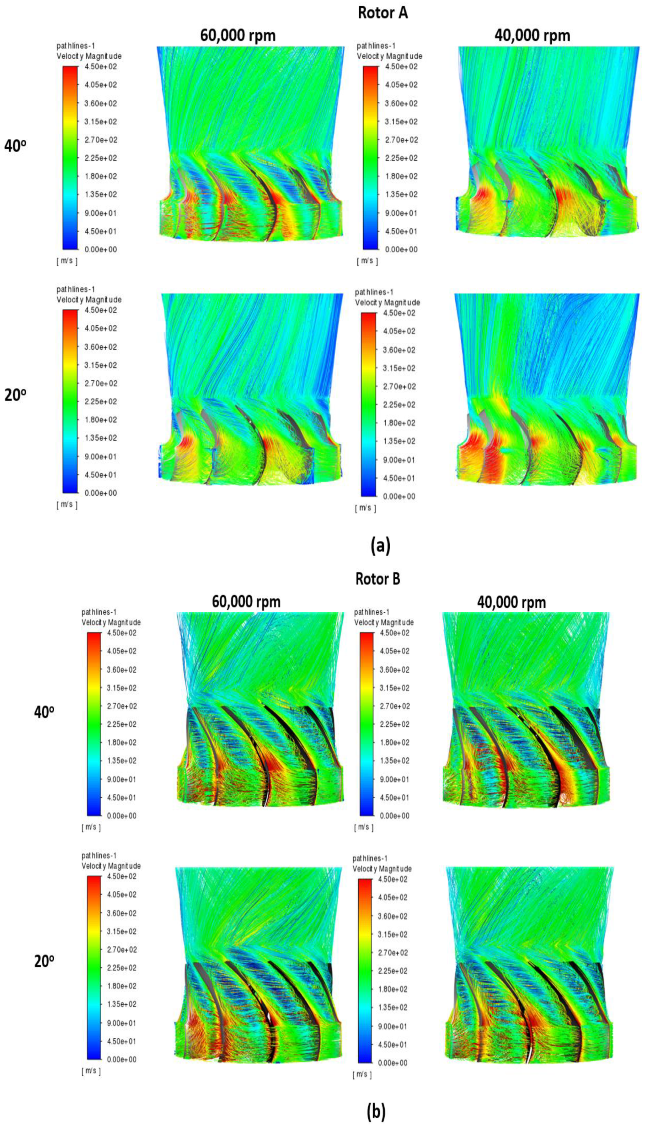
5.1. Separation of Exhaust Gases at the Inlet to the First-Stage Rotor
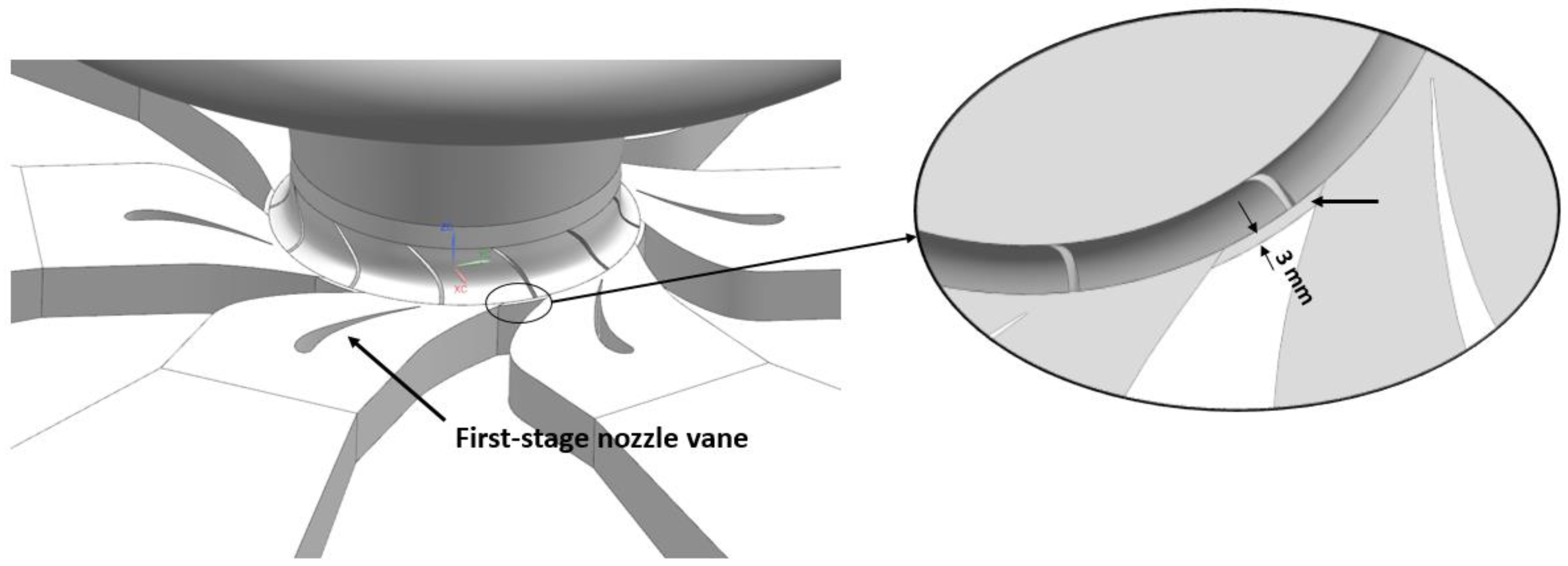
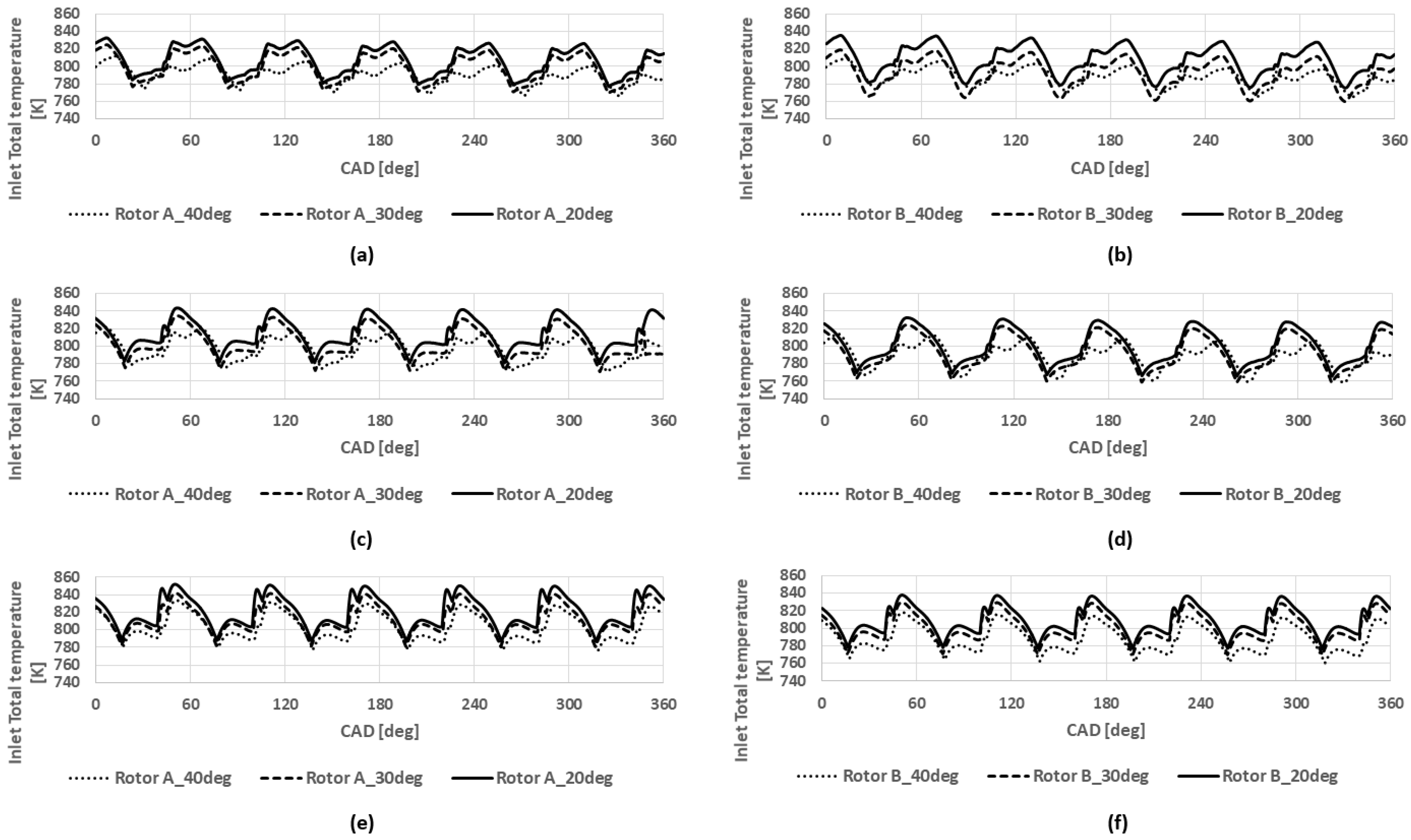
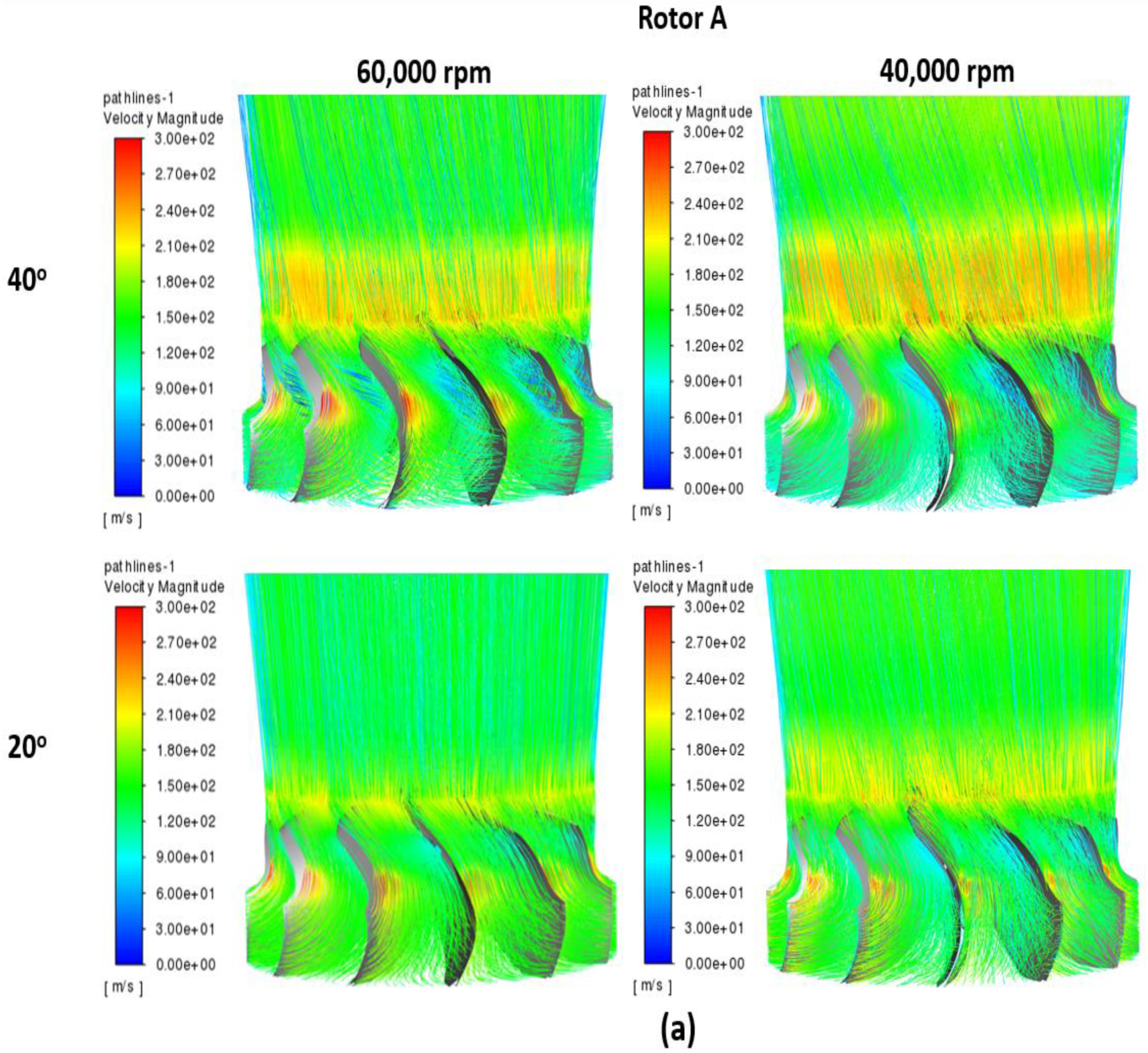
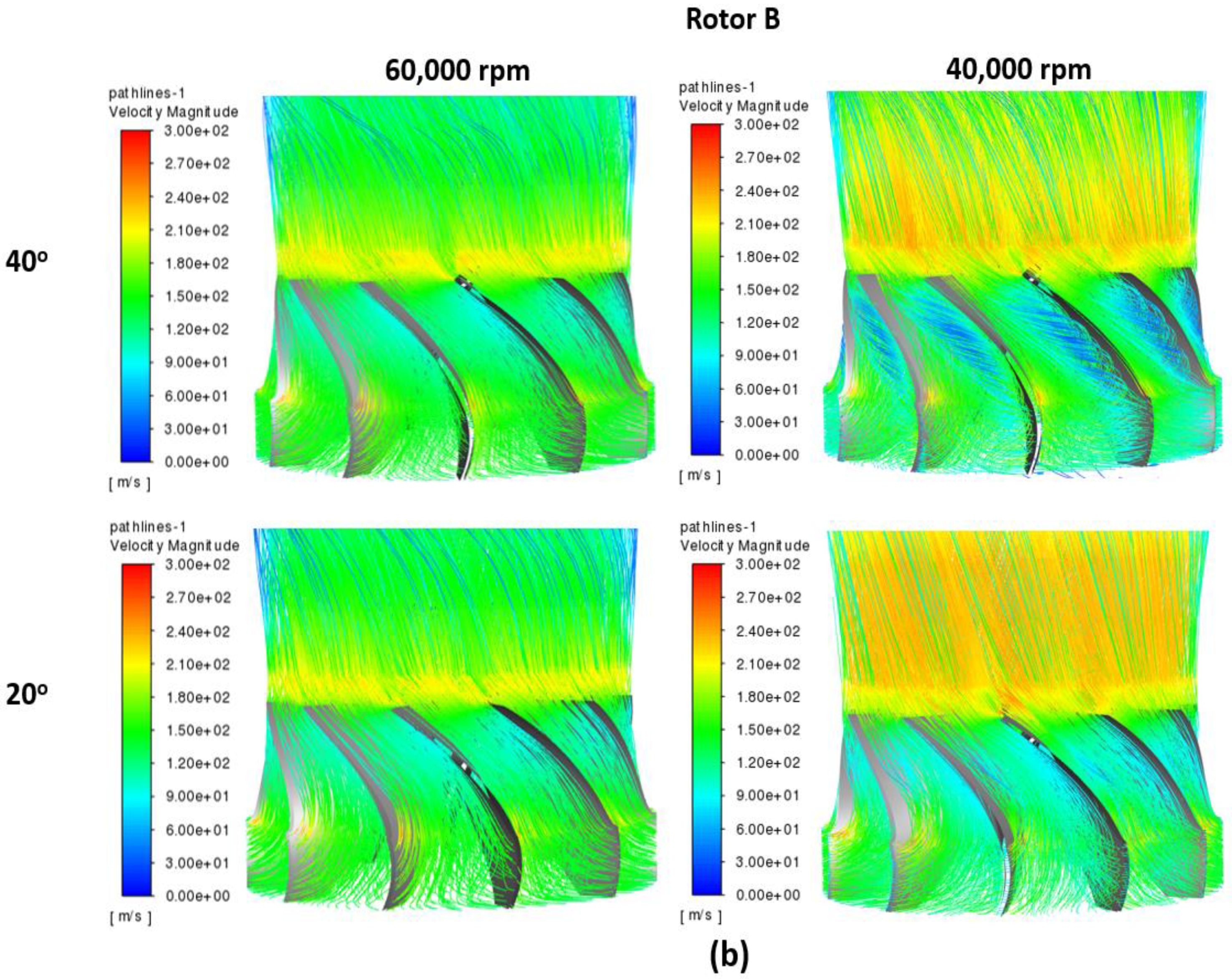
5.2. The Inlet to the First-Stage Rotor
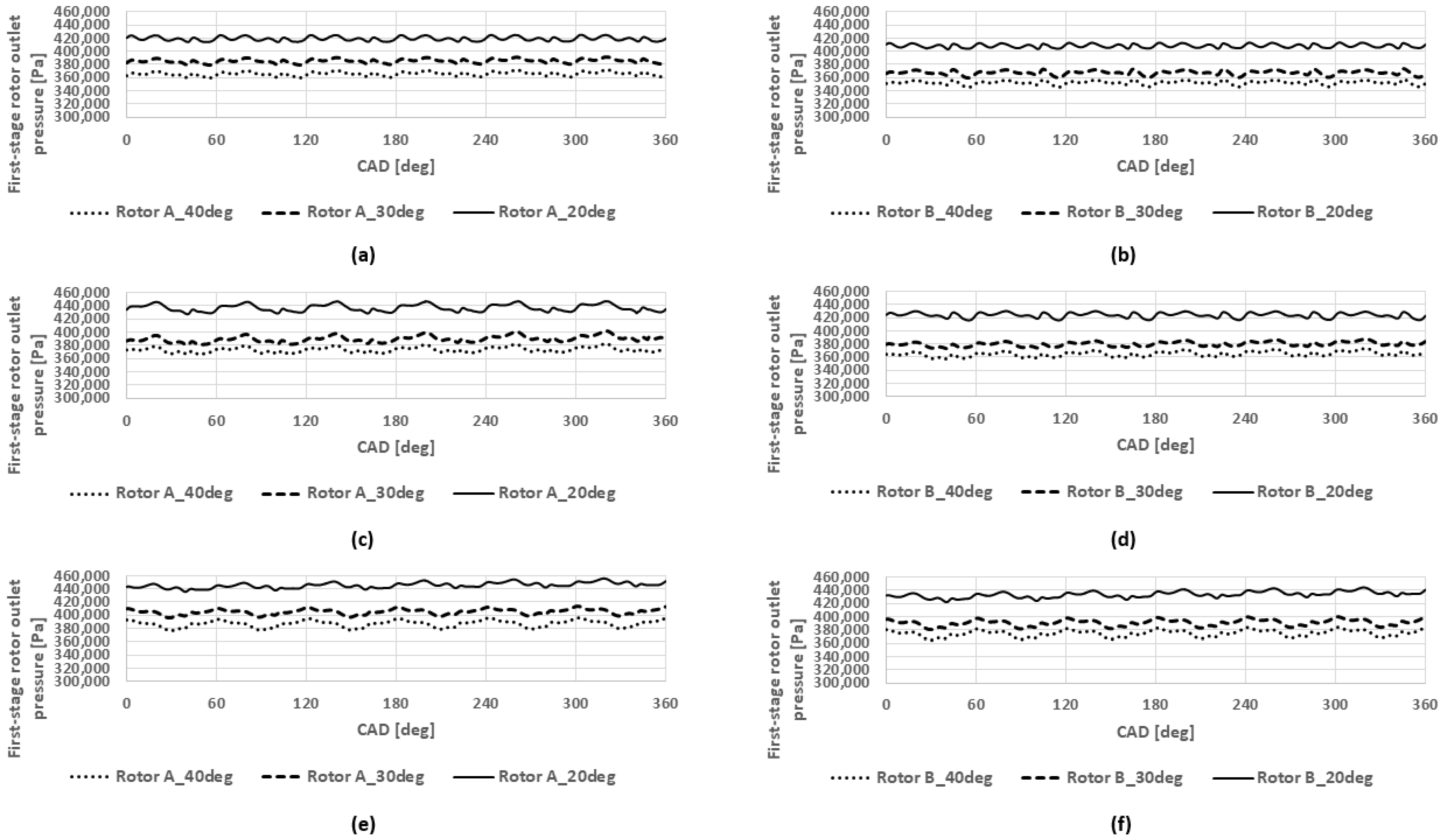
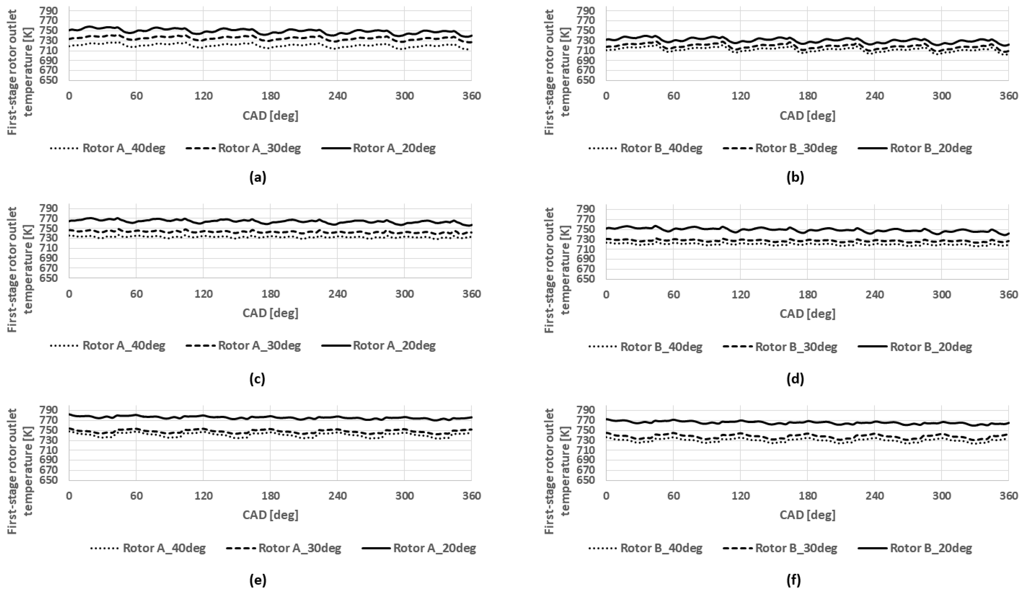
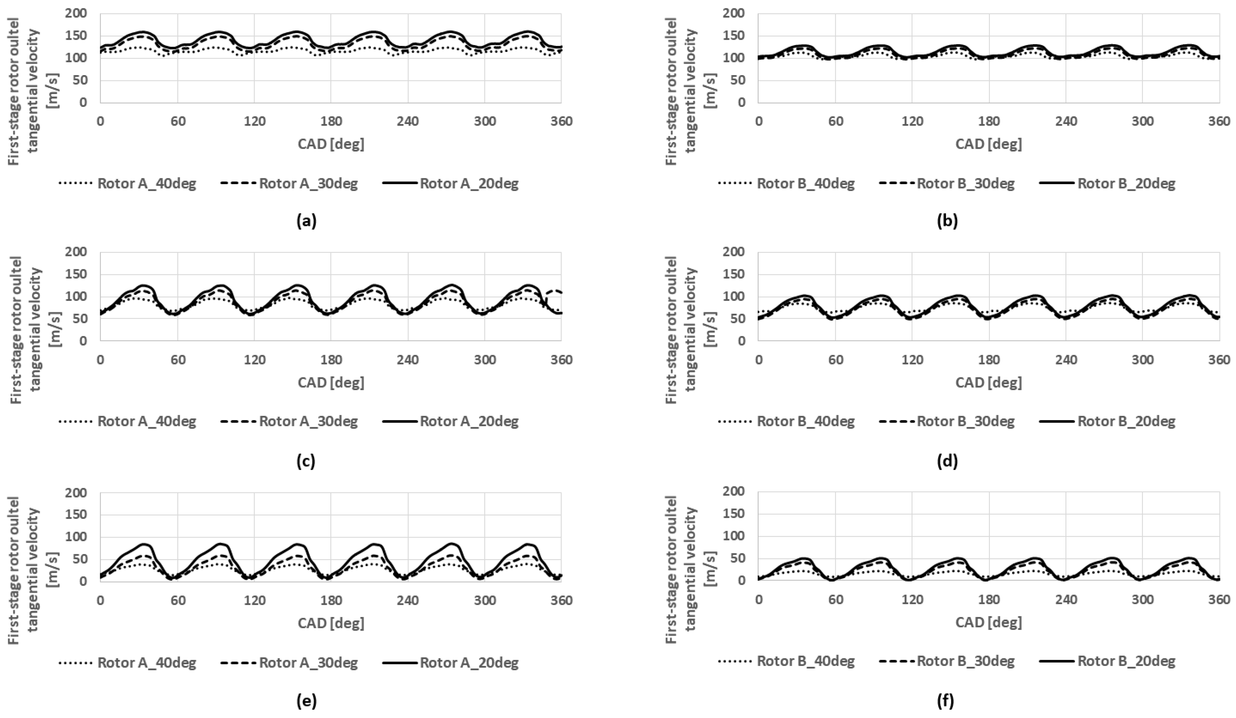
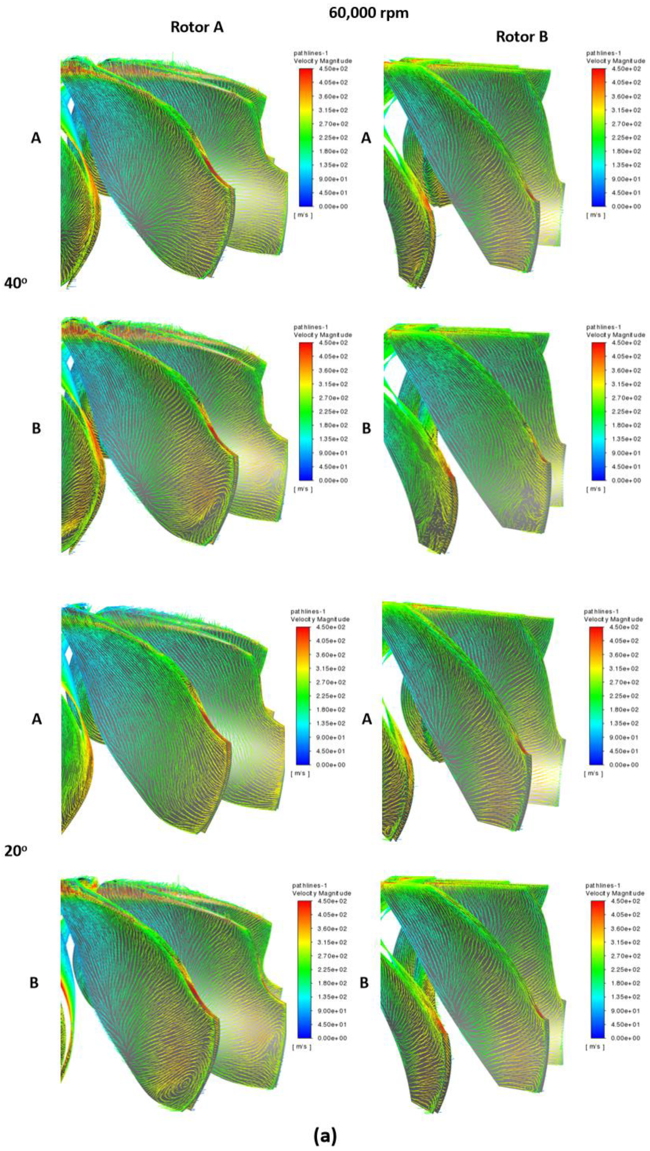
5.3. The Outlet from the First-Stage Rotor
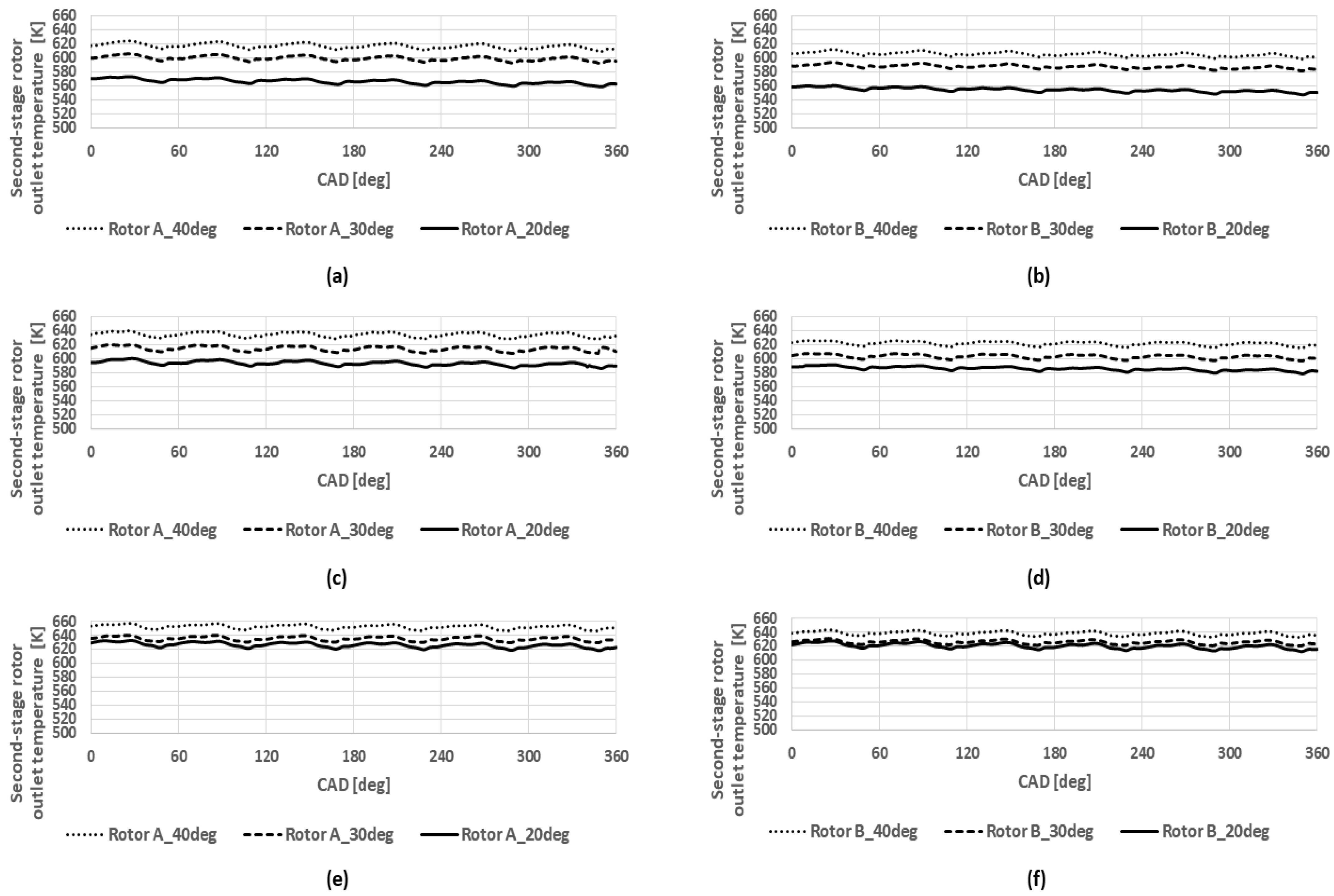
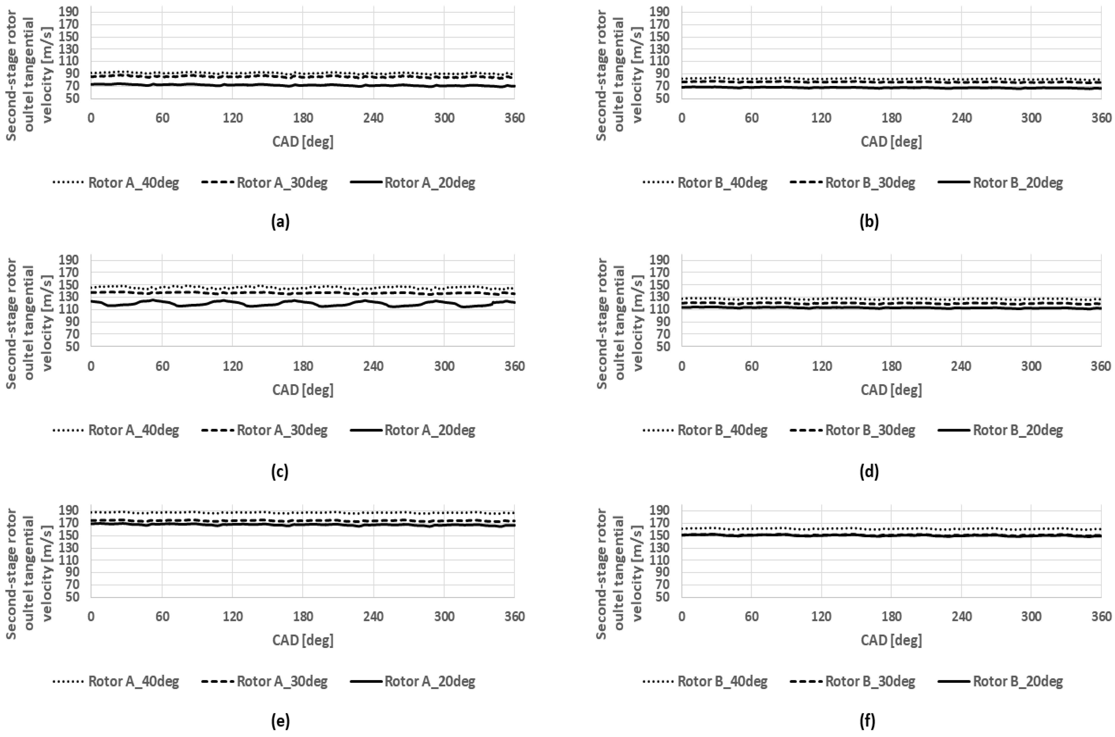
5.4. The Outlet from the Second-Stage Rotor
5.5. The Tangential Velocity Analysis
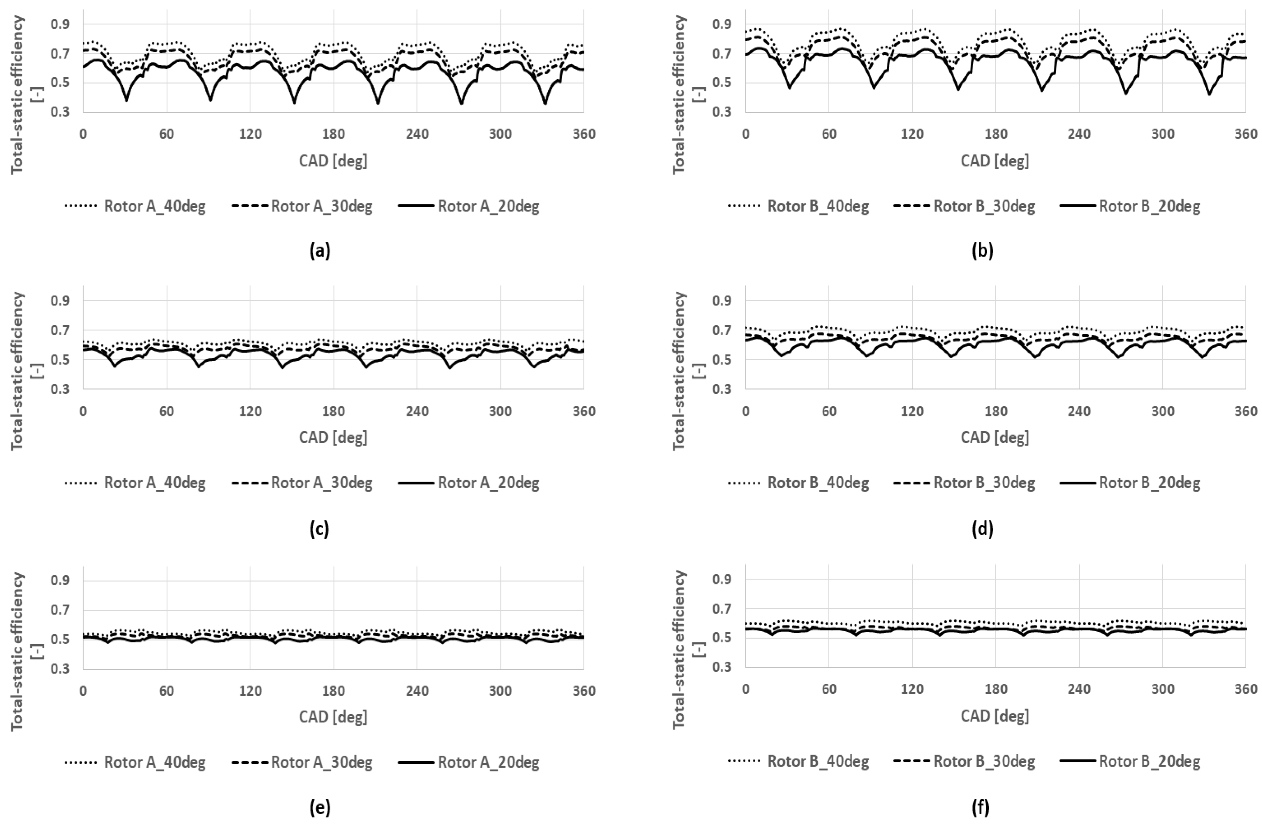
5.6. The Isentropic Efficiency of the First-Stage and Second-Stage Rotor
5.7. The Flow Losses at the First-Stage and Second-Stage Rotor
6. Conclusions
Author Contributions
Funding
Data Availability Statement
Acknowledgments
Conflicts of Interest
Nomenclature
| Notations | |
| w | Relative velocity |
| c | Absolute velocity |
| u | Linear velocity |
| Total enthalpy | |
| Turbine total-static efficiency | |
| X | Measured/observed value |
| n | Number of measurements |
| Turbine pressure-ratio | |
| p | Pressure |
| h | Static enthalpy |
| k′ | Heat capacity ratio of exhaust gases |
| R′ | Gas constant of exhaust gases |
| T* | Total temperature |
| Density | |
| t | Time |
| U | Vector of velocity |
| Molecular stress tensor | |
| Momentum source | |
| Thermal conductivity | |
| T | Static temperature |
| Energy source | |
| Position vector in tensor rotation | |
| Modified turbulent kinematic viscosity | |
| Production of turbulent viscosity | |
| S-A turbulence model constant | |
| S-A turbulence model constant | |
| Destruction of turbulent viscosity | |
| Source term | |
| Damping function | |
| Abbreviations | |
| ICE | Internal combustion engine |
| 3-D | Three-dimensional |
| 1-D | One-dimensional |
| LE | Leading edge |
| TE | Trailing edge |
| CAD | Crank angle degree |
| CFD | Computational fluid dynamics |
| VTG | Variable Turbine Geometry |
| RMSE | Root mean square error |
| St | Strouhal number |
| Subscripts | |
| 0 | Conditions at the rotor inlet |
| 1 | Conditions after first-stage nozzle vanes |
| 2 | Conditions after first-stage rotor |
| 3 | Conditions before second-stage rotor |
| 4 | Conditions after second-stage rotor |
| tot | Total |
References
- Nikita, C. Pulsating Flow Phenomena in Exhaust Manifolds. Ph.D. Thesis, Imperial College, London, UK, August 2017. [Google Scholar]
- Gopal, P.; Kumar, T.S.; Kumaragurubaran, B. Analysis of Flow through the Exhaust Manifold of a Multi Cylinder Petrol Engine for Improved Volumetric Efficiency. Int. J. Dyn. Fluids 2009, 5, 15. [Google Scholar]
- Poal, D.; Dwyer, M. A Simple Theory for Pressure Pulses in Exhaust Systems. Proc. Inst. Mech. Eng. 1964, 179, 365–394. [Google Scholar] [CrossRef]
- Semlitsch, B.; Wang, Y.; Mihăescu, M. Flow Effects due to Pulsation in an Internal Combustion Engine Exhaust Port. Energy Convers. Manag. 2014, 86, 520–536. [Google Scholar] [CrossRef] [Green Version]
- Hong, B.; Venkataraman, V.; Cronhjort, A. Numerical Analysis of Engine Exhaust Flow Parameters for Resolving Pre-Turbine Pulsating Flow Enthalpy and Exergy. Energies 2021, 14, 6183. [Google Scholar] [CrossRef]
- Serrano, J.; Arnau, F.; Gracía, L.; Samala, V.; Smith, L. Experimental Approach for the Characterization and Performance Analysis of Twin Entry Radial-Inflow Turbines in a Gas Stand and with Different Flow Admission Conditions. Appl. Therm. Eng. 2019, 159, 113737. [Google Scholar] [CrossRef]
- Usai, V.; Marelli, S. Steady State Experimental Characterization of a Twin Entry Turbine under Different Admission Conditions. Energies 2021, 14, 2228. [Google Scholar] [CrossRef]
- Copeland, D.; Martinez-Botas, R.; Seiler, M. Comparison Between Steady and Unsteady Double-Entry Turbine Performance Using the Quasi-Steady Assumption. ASME J. Turbomach. 2011, 133, 031001. [Google Scholar] [CrossRef]
- Marelli, S.; Capobianco, M. Steady and Pulsating Flow Efficiency of a Waste-Gated Turbocharger Radial Flow Turbine for Automotive Application. Energy 2011, 36, 459–465. [Google Scholar] [CrossRef]
- Chiong, M.; Rajoo, S.; Romagnoli, A.; Costall, A.; Martinez-Botas, R. One-Dimensional Pulse-Flow Modeling of a Twin-Scroll Turbine. Energy 2016, 115, 1291–1304. [Google Scholar] [CrossRef]
- Chen, H.; Hakeem, I.; Martinez-Botas, R. Modelling of a Turbocharger Turbine Under Pulsating Inlet Conditions. Proc. Inst. Mech. Eng. Part A J. Power Energy 1996, 210, 397–408. [Google Scholar] [CrossRef]
- Yang, M.; Deng, K.; Martines-Botas, R.; Zhuge, W. An Investigation on Unsteadiness of a Mixed-Flow Turbine Under Pulsating Conditions. Energy Convers. Manag. 2016, 110, 51–58. [Google Scholar] [CrossRef]
- Chiong, M.; Rajoo, S.; Romagnoli, A.; Costall, A.; Martinez-Botas, R. Non-Adiabatic Pressure Loss Boundary Condition for Modelling Turbocharger Turbine Pulsating Flow. Energy Convers. Manag. 2015, 93, 267–281. [Google Scholar] [CrossRef] [Green Version]
- Wang, H.; Chao, Y.; Tang, T.; Luo, K.; Qin, K. A Comparison of Partial Admission Axial and Radial Inflow Turbines for Underwater Vehicles. Energies 2021, 14, 1514. [Google Scholar] [CrossRef]
- Newton, P.; Copeland, C.; Martinez-Botas, R.; Seiler, M. An Audit of Aerodynamic Loss in a Double Entry Turbine under Full and Partial Admission. Int. J. Heat Fluid Flow 2012, 33, 70–80. [Google Scholar] [CrossRef] [Green Version]
- Copeland, C.; Newton, P.; Martinez-Botas, R.; Seiler, M. A Comparison of Timescales within a Pulsed Flow Turbocharger Turbine. In Proceedings of the Institution of Mechanical Engineers—10th International Conference on Turbochargers and Turbocharging, London, UK, 15–16 May 2012. [Google Scholar]
- Yang, B.; Martinez-Botas, R.; Yang, M. Rotor Flow-Field Timescale and Unsteady Effects on Pulsed-Flow Turbocharger Turbine. Aerosp. Sci. Technol. 2022, 120, 107231. [Google Scholar] [CrossRef]
- Xue, Y.; Yang, M.; Martinez-Botas, R.; Yang, B.; Deng, K. Unsteady Performance of a Mixed-Flow Turbine with Nozzled Twin-Entry Volute Confronted by Pulsating Incoming Flow. Aerosp. Sci. Technol. 2019, 95, 105485. [Google Scholar] [CrossRef]
- Cerdoun, M.; Ghenaiet, A. Unsteady Behavior of a Twin Entry Radial Turbine under Engine Like Inlet Flow Conditions. Appl. Therm. Eng. 2018, 130, 93–111. [Google Scholar] [CrossRef]
- Padzillah, M.; Rajoo, S.; Martinez-Botas, R. Influence of Speed and Frequency towards the Automotive Turbocharger Turbine Performance under Pulsating Flow Conditions. Energy Convers. Manag. 2014, 80, 416–428. [Google Scholar] [CrossRef]
- Fürst, J.; Zak, Z. Numerical Simulation of Unsteady Flows Through a Radial Turbine. Adv. Comput. Math. 2019, 45, 1939–1952. [Google Scholar] [CrossRef]
- Hassan, A.; Fuhrer, C.; Schatz, M.; Vogt, D. Multi-channel Casing Design for Radial Turbine Operation Control. In Proceedings of the 13th European Conference on Turbomachinery Fluid Dynamics & Thermodynamics ETC13, Lausanne, Switzerland, 8–12 April 2019. [Google Scholar] [CrossRef]
- Zhao, R.; Li, W.; Zhuge, W.; Zhang, Y. Unsteady Flow Loss Mechanism and Aerodynamic Improvement of Two-Stage Turbine under Pulsating Conditions. Entropy 2019, 21, 985. [Google Scholar] [CrossRef]
- BorgWarner Performance Turbochargers Catalog. Available online: https://images.carid.com/borgwarner/info/pdf/airwerks-intro.pdf (accessed on 16 November 2022).
- Zahed, A.; Bayomi, N. Radial Turbine Design Process. ISESCO J. Sci. Technol. 2015, 11, 9–22. [Google Scholar]
- Continuity and Momentum Equations. Available online: https://www.afs.enea.it/project/neptunius/docs/fluent/html/th/node11.htm (accessed on 19 December 2022).
- Kozak, D.; Mazuro, P.; Teodorczyk, A. Numerical Simulation of Two-Stage Variable Geometry Turbine. Energies 2021, 14, 5349. [Google Scholar] [CrossRef]
- Galindo, J.; Fajardo, P.; Navarro, R.; Garcia-Cuevas, L. Characterization of a Radial Turbocharger Turbine in Pulsating Flow by Means of CFD and its Application to Engine Modeling. Appl. Energy 2013, 103, 116–127. [Google Scholar] [CrossRef]
- Spalart, P.; Allmaras, S. A One-Equation Turbulence Model for Aerodynamic Flows. Rech. Aerosp. 1994, 1, 5–21. [Google Scholar] [CrossRef]
- Zhang, Y.; Chen, L.; Zhuge, W.; Zhang, S. Effects of Pulse Flow and Leading Edge Sweep on Mixed Flow Turbines for Engine Exhaust Heat Recovery. Sci. China Technol. Sci. 2011, 54, 295–301. [Google Scholar] [CrossRef]
- Yang, M.; Martinez-Botas, R.; Rajoo, S.; Yokoyama, T.; Ibaraki, S. An Investigation of Volute Cross-Sectional Shape on Turbocharger Turbine Under Pulsating Conditions in Internal Combustion Engine. Energy Convers. Manag. 2015, 105, 167–177. [Google Scholar] [CrossRef] [Green Version]
- Transport Equation for the Spalart-Allmaras Model. Available online: https://www.afs.enea.it/project/neptunius/docs/fluent/html/th/node50.htm (accessed on 19 December 2022).
- Hassan, A.; Schatz, M.; Vogt, A. Performance and Losses Analysis for Radial Turbine Featuring a Multi-Channel Casing Design. J. Turbomach. 2021, 143, 021003. [Google Scholar] [CrossRef]
- Anton, N.; Birkestad, P. The 6-Inlet Single Stage Axial Turbine Concept for Pulse-Turbocharging: A Numerical Investigation; SAE Technical Paper; SAE: Warrendale, PA, USA, 2019. [Google Scholar] [CrossRef]


| Rotor A | |
| Inlet diameter (m) | 0.140 |
| Outlet diameter (m) | 0.125 |
| Number of blades | 12 |
| Maximal rotor speed (rpm) | 68,500 |
| Maximal pressure ratio (-) | 4.4 |
| Maximal mass flow rate (kg/s) | 1.45 |
| Rotor B | |
| Inlet diameter (m) | 0.11 |
| Outlet diameter (m) | 0.10 |
| Number of blades | 11 |
| Maximal rotor speed (rpm) | 97,000 |
| Maximal pressure ratio (-) | 4.8 |
| Maximal mass flow rate (kg/s) | 1.15 |
| Engine Parameters | |
|---|---|
| Number of cylinders | |
| Type | 2-stroke |
| Rotational speed | 1500 |
| Cylinder bore (mm) | 115 |
| Cylinder Stroke (mm) | 195.2 |
| Displacement (cm3) | 24,000 |
| Crankshaft angle step (deg) | 0.1 |
| Case | Turbine Speed n (rpm) | VTG Vane Positions (deg) |
|---|---|---|
| 1 | 40,000 | 20 |
| 2 | 30 | |
| 3 | 40 | |
| 4 | 50,000 | 20 |
| 5 | 30 | |
| 6 | 40 | |
| 7 | 60,000 | 20 |
| 8 | 30 | |
| 9 | 40 |
| Inlet Boundary Condition | |
| Boundary condition type | Mass-flow rate |
| Mass-flow rate values (kg/s) | 0 ÷ 1.5 |
| Inlet temperature (K) | 700 |
| Gauge-pressure (Pa) | 300,000 |
| Outlet Boundary Condition | |
| Boundary condition type | Pressure outlet |
| Outlet pressure (Pa) | 100,000 |
| Outlet temperature (K) | 500 |
| Rotor A | |
| Exhaust pipes domain (×6) | 64,800 |
| First-stage rotor domain | 1,295,900 |
| Diffuser domain | 55,200 |
| Inter-stage pipes domain | 536,390 |
| Second-stage rotor domain | 1,230,600 |
| Outlet domain | 63,000 |
| Total number of elements | 3,245,890 |
| Rotor B | |
| Exhaust pipes domain (×6) | 64,800 |
| First-stage rotor domain | 1,310,900 |
| Diffuser domain | 55,200 |
| Inter-stage pipes domain | 536,390 |
| Second-stage rotor domain | 1,324,000 |
| Outlet domain | 63,000 |
| Total number of elements | 3,354,290 |
| Computational Machine | |
|---|---|
| Central Processing Unit (CPU) type | Ryzen 9 |
| Number of CPU cores | 9 |
| Random-Access Memory (RAM) (Gb) | 128 |
| Rotor A | Rotor B | ||||
|---|---|---|---|---|---|
| Turbine Speed (rpm) | VTG Vanes Angle (deg) | Exhaust Mass-Flow Rate (kg/s) | Turbine Speed (rpm) | VTG Vanes Angle (deg) | Exhaust Mass-Flow Rate (kg/s) |
| 60,000 | 40 | 0.094 | 60,000 | 40 | 0.087 |
| 30 | 0.099 | 30 | 0.091 | ||
| 20 | 0.101 | 20 | 0.094 | ||
| 50,000 | 40 | 0.068 | 50,000 | 40 | 0.070 |
| 30 | 0.075 | 30 | 0.074 | ||
| 20 | 0.078 | 20 | 0.075 | ||
| 40,000 | 40 | 0.031 | 40,000 | 40 | 0.029 |
| 30 | 0.032 | 30 | 0.031 | ||
| 20 | 0.037 | 20 | 0.033 | ||
| Rotor A | Rotor B | ||||
|---|---|---|---|---|---|
| Turbine Speed (rpm) | VTG Vanes Angle (deg) | Average Pressure Ratio (-) | Turbine Speed (rpm) | VTG Vanes Angle (deg) | Average Pressure Ratio (-) |
| 60,000 | 40 | 1.72 | 60,000 | 40 | 1.80 |
| 30 | 1.68 | 30 | 1.77 | ||
| 20 | 1.66 | 20 | 1.71 | ||
| 50,000 | 40 | 1.59 | 50,000 | 40 | 1.63 |
| 30 | 1.57 | 30 | 1.62 | ||
| 20 | 1.54 | 20 | 1.56 | ||
| 40,000 | 40 | 1.42 | 40,000 | 40 | 1.53 |
| 30 | 1.41 | 30 | 1.52 | ||
| 20 | 1.38 | 20 | 1.45 | ||
| Rotor A | Rotor B | ||||
|---|---|---|---|---|---|
| Turbine Speed (rpm) | VTG Vanes Angle (deg) | Average Temperature Drop (K) | Turbine Speed (rpm) | VTG Vanes Angle (deg) | Average Temperature Drop (K) |
| 60,000 | 40 | 69.80 | 60,000 | 40 | 77.77 |
| 30 | 63.56 | 30 | 72.59 | ||
| 20 | 57.28 | 20 | 76.67 | ||
| 50,000 | 40 | 64.15 | 50,000 | 40 | 69.71 |
| 30 | 58.73 | 30 | 64.56 | ||
| 20 | 49.35 | 20 | 51.04 | ||
| 40,000 | 40 | 62.45 | 40,000 | 40 | 65.26 |
| 30 | 64.59 | 30 | 69.96 | ||
| 20 | 44.71 | 20 | 49.70 | ||
| Rotor A | Rotor B | ||||
|---|---|---|---|---|---|
| Turbine Speed (rpm) | VTG Vanes Angle (deg) | Average Pressure Ratio (-) | Turbine Speed (rpm) | VTG Vanes Angle (deg) | Average Pressure Ratio (-) |
| 60,000 | 40 | 2.23 | 60,000 | 40 | 3.07 |
| 30 | 2.58 | 30 | 3.13 | ||
| 20 | 3.41 | 20 | 3.62 | ||
| 50,000 | 40 | 2.16 | 50,000 | 40 | 3.17 |
| 30 | 2.49 | 30 | 3.08 | ||
| 20 | 3.02 | 20 | 3.22 | ||
| 40,000 | 40 | 2.17 | 40,000 | 40 | 2.94 |
| 30 | 2.36 | 30 | 2.91 | ||
| 20 | 2.87 | 20 | 3.14 | ||
| Rotor A | Rotor B | ||||
|---|---|---|---|---|---|
| Turbine Speed (rpm) | VTG Vanes Angle (deg) | Average Temperature Drop (K) | Turbine Speed (rpm) | VTG Vanes Angle (deg) | Average Temperature Drop (K) |
| 60,000 | 40 | 84.85 | 60,000 | 40 | 131.37 |
| 30 | 118.21 | 30 | 155.69 | ||
| 20 | 166.36 | 20 | 167.60 | ||
| 50,000 | 40 | 79.63 | 50,000 | 40 | 123.28 |
| 30 | 110.32 | 30 | 148.15 | ||
| 20 | 152.88 | 20 | 169.60 | ||
| 40,000 | 40 | 69.33 | 40,000 | 40 | 110.04 |
| 30 | 92.84 | 30 | 129.56 | ||
| 20 | 130.84 | 20 | 157.74 | ||
| Rotor A | Rotor B | ||||
|---|---|---|---|---|---|
| Turbine Speed (rpm) | VTG Vanes Angle (deg) | Average Tangential Velocity (m/s) | Turbine Speed (rpm) | VTG Vanes Angle (deg) | Average Tangential Velocity (m/s) |
| 60,000 | 40 | 116.90 | 60,000 | 40 | 105.92 |
| 30 | 132.98 | 30 | 109.31 | ||
| 20 | 141.19 | 20 | 114.77 | ||
| 50,000 | 40 | 82.82 | 50,000 | 40 | 74.45 |
| 30 | 88.22 | 30 | 73.17 | ||
| 20 | 93.94 | 20 | 79.03 | ||
| 40,000 | 40 | 27.11 | 40,000 | 40 | 15.91 |
| 30 | 34.15 | 30 | 21.86 | ||
| 20 | 48.57 | 20 | 27.32 | ||
| Rotor A | Rotor B | ||||
|---|---|---|---|---|---|
| Turbine Speed (rpm) | VTG Vanes Angle (deg) | Average Tangential Velocity (m/s) | Turbine Speed (rpm) | VTG Vanes Angle (deg) | Average Tangential Velocity (m/s) |
| 60,000 | 40 | 91.11 | 60,000 | 40 | 81.71 |
| 30 | 85.29 | 30 | 76.50 | ||
| 20 | 71.78 | 20 | 67.67 | ||
| 50,000 | 40 | 145.88 | 50,000 | 40 | 127.74 |
| 30 | 137.62 | 30 | 119.58 | ||
| 20 | 119.68 | 20 | 113.00 | ||
| 40,000 | 40 | 187.25 | 40,000 | 40 | 161.13 |
| 30 | 174.32 | 30 | 150.84 | ||
| 20 | 168.04 | 20 | 150.51 | ||
| Rotor A | Rotor B | ||||
|---|---|---|---|---|---|
| Turbine Speed (rpm) | VTG Vanes Angle (deg) | Average Total-Static Efficiency (-) | Turbine Speed (rpm) | VTG Vanes Angle (deg) | Average Total-Static Efficiency (-) |
| 60,000 | 40 | 0.71 | 60,000 | 40 | 0.78 |
| 30 | 0.66 | 30 | 0.73 | ||
| 20 | 0.57 | 20 | 0.64 | ||
| 50,000 | 40 | 0.61 | 50,000 | 40 | 0.69 |
| 30 | 0.58 | 30 | 0.65 | ||
| 20 | 0.53 | 20 | 0.60 | ||
| 40,000 | 40 | 0.55 | 40,000 | 40 | 0.61 |
| 30 | 0.53 | 30 | 0.57 | ||
| 20 | 0.51 | 20 | 0.55 | ||
| Rotor A | Rotor B | ||||
|---|---|---|---|---|---|
| Turbine Speed (rpm) | VTG Vanes Angle (deg) | Average Total-Static Efficiency (-) | Turbine Speed (rpm) | VTG Vanes Angle (deg) | Average Total-Static Efficiency (-) |
| 60,000 | 40 | 0.60 | 60,000 | 40 | 0.66 |
| 30 | 0.75 | 30 | 0.80 | ||
| 20 | 0.84 | 20 | 0.89 | ||
| 50,000 | 40 | 0.46 | 50,000 | 40 | 0.53 |
| 30 | 0.58 | 30 | 0.67 | ||
| 20 | 0.73 | 20 | 0.78 | ||
| 40,000 | 40 | 0.43 | 40,000 | 40 | 0.47 |
| 30 | 0.52 | 30 | 0.60 | ||
| 20 | 0.63 | 20 | 0.69 | ||
Disclaimer/Publisher’s Note: The statements, opinions and data contained in all publications are solely those of the individual author(s) and contributor(s) and not of MDPI and/or the editor(s). MDPI and/or the editor(s) disclaim responsibility for any injury to people or property resulting from any ideas, methods, instructions or products referred to in the content. |
© 2023 by the authors. Licensee MDPI, Basel, Switzerland. This article is an open access article distributed under the terms and conditions of the Creative Commons Attribution (CC BY) license (https://creativecommons.org/licenses/by/4.0/).
Share and Cite
Kozak, D.; Mazuro, P. Numerical Analysis of Two-Stage Turbine System for Multicylinder Engine under Pulse Flow Conditions with High Pressure-Ratio Turbine Rotor. Energies 2023, 16, 751. https://doi.org/10.3390/en16020751
Kozak D, Mazuro P. Numerical Analysis of Two-Stage Turbine System for Multicylinder Engine under Pulse Flow Conditions with High Pressure-Ratio Turbine Rotor. Energies. 2023; 16(2):751. https://doi.org/10.3390/en16020751
Chicago/Turabian StyleKozak, Dariusz, and Paweł Mazuro. 2023. "Numerical Analysis of Two-Stage Turbine System for Multicylinder Engine under Pulse Flow Conditions with High Pressure-Ratio Turbine Rotor" Energies 16, no. 2: 751. https://doi.org/10.3390/en16020751