Contaminant Transport from a Deep Geological Repository: Lumped Parameters Derived from a 3D Hydrogeological Model

Abstract

A model of contaminant transport from a repository to the biosphere is one of the major needs in the safety assessment of the geological disposal of spent nuclear fuel. This work deals with the development of a procedure that obtained characteristic data from the transport path by postprocessing the results of the 3D flow and transport models, according to the repository concept for the Czech Republic. Postprocessing was used to map the entire transport pathway, which included the smallest tracer flows; therefore, it is called the “integral method”. The results are the characteristics of the storage system, such as: transport path length, flow time, total dilution, groundwater flow, longitudinal dispersivity, porosity, etc. These acquired characteristics can be used directly in safety analyses or to narrow the selection of candidate sites. Furthermore, these parameters were used to set up a model with lumped parameters (in this case, created in the GoldSim SW environment). Even only one “Pipe” component, after being properly set up, shows almost identical results to the entire 3D model. Based on the results of the 3D model, it is possible to set up a lumped parameter model that accurately simulates the transport path and can perform further calculations of a larger number of contaminants in repeated runs, e.g., with stochastic input data, which would be very laborious (or not possible at all) with the 3D model.

1. Introduction

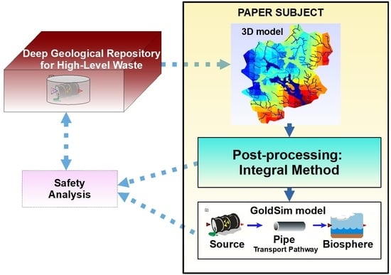
A generally considered plan for spent nuclear fuel (SNF) from a nuclear power plant involves geological disposal—placing the SNF deep underground with a system of engineered barriers and in stable low-permeable rocks as the natural barrier (geological barrier, geosphere). The safety assessment (SA) of the deep geological repository (DGR) depends on the radionuclide transport model through the system of barriers with the final output in the form of a radioactivity dose to humans within the biosphere. In this paper, we focused on the geosphere radionuclide transport model in crystalline rock and its role in the SA and site selection process. The model considers, in general, the temporal evolution of the radionuclide (contaminant) flux as the input and the temporal evolution of the flux from the geosphere to the biosphere as the output. The input flux is meant as the flux from the engineered barrier to the geosphere, but within the explanation in this paper, we cover the whole source system under the term “repository”. From such a “far-field” context, the time period after at least 1000 years is relevant—until this time, canisters are not supposed to break and the heat effect of the spent fuel decreases significantly.

The context of the model used can be multiple. To prove the repository safety, it is required to verify that the output activity flux is below a certain limit (to fulfill the consequential limits on the annual effective dose). To select the repository location among several candidates, the model can support the decision either by ranking the resulting dose criterion (minimal) or looking at other conditions and the cost-effectiveness under the given constraint of the dose limit. For both cases, it is convenient that the transport model can be evaluated with small computing costs (e.g., time) and that it is represented by a small set of parameters that have intuitive physical meaning and provide worse/better classifications for the DGR performance. A quick calculation is a necessity for stochastic modeling considering statistical distributions (or in general uncertainty) of the input parameters.

The lumped parameter model (LPM) is a term for representing a system as a whole, by a small number of global parameters and the interaction through, e.g., “input” and “output”, typically as ordinary differential equations, as opposed to distributed parameter models, with partial differential equations, which are typical cases of groundwater flow and solute transport models with realistic aquifer geometry and geological heterogeneity, boundary conditions, solved by numerical methods. An example of LPM in the contaminant transport and safety assessment context is the compartment concept in GoldSim software [1]—the basic “Pipe” object represents the 1D channel with advection, diffusion, and other interactions, in which homogeneous (lumped) parameters are evaluated by the analytical solution. A similar approach is applied in [2].

LPMs are typically used in DGR SA projects, particularly for the reasons mentioned above. Historically, the models were set as abstraction or conceptualization of the real hydrogeological systems (Figure 1)—the geometrical and material parameters and fluxes could be obtained by rough estimates [3]. Various terms are used in this context, such as “compartment model” [4] or “simplified representative model” [5]. Besides this, 3D groundwater numerical models are almost standard, mostly achievable by desktop PCs, and limited by geological data rather than by computing power. Gradual improvements of radionuclide transport models in the US program of the DGR development are documented in [6].

Although 3D models with detailed geologies for the respective research laboratories or candidate sites are set, the links between them and the LPMs do not garner much attention. A compartment model [7] in the Czech DGR program does not include far-field hydrogeological data. The CYDER model [8] is verified against another compartment-type model. Within the Swedish program, the earlier study with CHAN3D actually represented realistic fracture networks, but for the SA application [9], it was used with a high level of abstraction (to fractures as system components). Current SA models [4] derive parameters of the compartment model by means of the particle tracking method with the detailed groundwater flow model—with this, individual pathways are obtained, with the advective travel time and transport resistance (F-factor) as parameters. The latter parameter is linked to individual fracture geometry and the concept does not capture the effects of the whole flow field, including dispersion. Another work [10] focuses on particle tracking improvement for fracture–continuum models. The Korean model [11] uses GoldSim software, but the geosphere compartment parameters are examples only and are not linked to detailed hydrogeological models.

There are works on LPM in other groundwater applications, with similar motivations, some of them also focus on aspects of LPM and real system comparisons. Given the residence time distribution (RTD) of the original system, the model RTDMM [12] consists of a sequence of control volumes that can be represented as 1D numerical discretization. This more generic configuration allows a more accurate representation than strictly defined LPM. However, it is not aimed to provide characteristics that could also be used as lumped parameters and as safety indicators. The RTD is considered as input for the method, not the original 3D groundwater model. A model for the nitrate pollution vulnerability of groundwater in sedimentary aquifers [13] highlights the utility of two parameters derived from a natural water age tracer (field sampling) as the vulnerability indicator. A lumped model of fresh/saline water mixing in coastal lowlands RSGEM [14], used to support operational water management, was successfully compared to both field data and a complex numerical groundwater model. The use of LPMs within Monte Carlo simulations, with a large number of repeated model runs, is shown in [15,16].

The purpose of this work was to introduce a procedure to derive a set of lumped parameters (of the geosphere as one of the DGR barriers) from a 3D flow and transport model containing the available hydrogeological knowledge of a particular repository site. This would be more general than [4]; more potentially relevant parameters are obtained, which can have the meaning of either safety/performance indicators or inputs to the “pipe” model of contaminant transport for quick evaluation. This procedure defines the LPM as an upscaling of the original 3D model and helps justify the compartment-like models for SA, which could not be available with the concept of [4], where the processes of dispersion and retention are added to the compartment model separately. The calculation is based on integral operations with the flow and solute transport model results, comprising virtually all of the pathways; therefore, the term “integral method” is suggested, distinguishing from the case of particle pathways [4,10]. Geometric and mass balance relationships are combined with the analysis of residence time distribution moments from the Dirac tracer input.

While the concept and technical procedures are generic, the demonstration of use and verification were done with two software codes as representative examples. Flow123d [17] software, an in-house developed open-source code, was used for calculations of 3D models. For derived LPM, the commercial GoldSim software environment was used with its “pipe” object.

The method was demonstrated on data from a Czech DGR candidate site. Although the data were provided directly from the site models elaborated for SÚRAO, the national authority [18,19], this study is not a part of the official site selection process. Therefore, the sites were used anonymously, and the data can be subject to perturbation. The presented indicator values and site rankings are the meanings of the method demonstration and testing.

The paper is structured as follows: The methods are described in Section 2 and Section 3, in particular the 3D model used as the input, the LPM as the desired upscaling, and the procedure of obtaining its parameters. The two related outputs of the work are presented in Section 4 and Section 6—the former involves the use of the obtained parameters for site ordering and the latter is the actual LPM formulation, calculation, and verification against the input 3D model. Then the conclusions section summarizes the applicability of the results, including the discussion of the LPM variants.

Some Basic Notions

Although the paper is not focused on performing the SA, to prepare a part of the necessary input data for it, it is useful to recall the considered meaning of a few basic terms related to DGR SA, based on the PAMINA international project [3]. Indicators are descriptive quantities that characterize the behavior of the disposal system and indicate whether it corresponds to the design. Performance indicators and safety indicators are introduced; the former corresponds to the use in this paper, where the geological barrier is considered as one SA component. Criterion narrows the sense of the indicator. The criterion is expressed by a single numerical value that can be checked against a given limit (while the indicator can be expressed quantitatively or with a range of values). Moreover, a generic meaning of “criterion” is used in this paper in the context of the optimization method (i.e., the objective function).

2. Used Data and Models

The concept of work assumes that a standard 3D numerical model of the DGR site is built, including all hydrogeological and other related data. It includes the use of the digital terrain model, specification of geological heterogeneity (rock type blocks or layers, faults as 2D planar subdomains), the definition of the boundary conditions eventually defining the infiltration and drainage areas, river positions, precipitation distribution, etc. (see Document S1). The interface between the repository volume and the geosphere must be defined in the model mesh or geometry. The models adopted from [18,19] represent DGRs in granite and are typically several kilometers large with meshes containing 1–2 million elements.

For examples in this work, models made with the Flow123d software [17] and their results were used. In principle, the method can be applied to any other numerical code where parameters and raw results linked to individual discretization elements are available in open-format files, or, e.g., through a simulation code owns’ scripting or an external interface.

The above-cited 3D models were built as follows, representing a long-term stable state after the near-field effects disappear: The boundaries in the plan view were defined along the water divides. The top surface was defined by a digital terrain model with a resolution of 10 m. The bottom boundary was defined at 1000 m depth (with respect to the lowest point of the surface). Depth-dependent hydraulic conductivity and porosity were used based on either local borehole measurements or generic Bohemian massif data. Faults were included in the models as 2D vertical structures with assigned transmissivity and porosity. The repository was included in the domain in the 500 m depth as a block size/dimensions of 1.8 km × 1.6 km × 50 m. Zero water and contaminant flow were prescribed on the lateral and bottom boundaries. The top boundary was distinguished between recharge and discharge boundaries. The selected element sides were defined as rivers with prescribed water levels at the surface, while the flow rate of 95–100 mm/a, corresponding to a defined share of precipitation, was prescribed on the remaining area. Subareas belonging to individual river basins were assigned. A zero contaminant (tracer) concentration was prescribed in the initial condition and the recharge flow. In the repository volume, a constant tracer concentration was prescribed (details below).

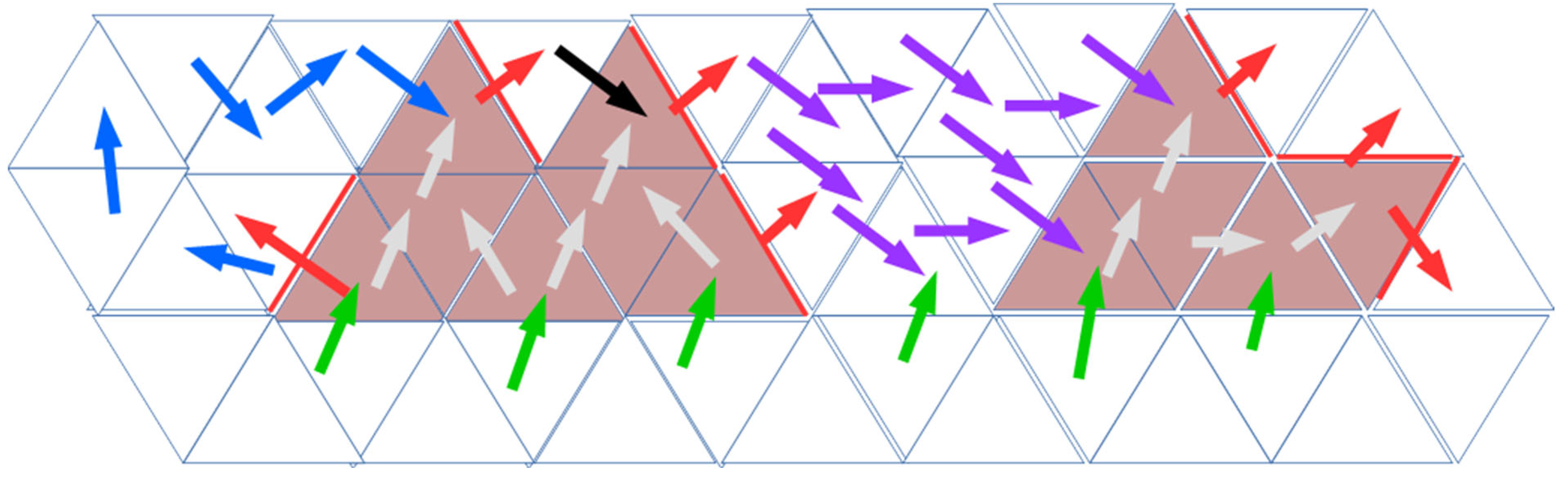
The configuration with the repository as a homogenized “porous rock” block with a prescribed concentration, a “backflow”, could occur in the block for three reasons: The first case could occur if the storage space is not continuous and has multiple parts (purple arrows in Figure 2). The second case (blue arrows in Figure 2 and white arrows in Figure 3) is caused by curved groundwater flow lines (topography and heterogeneity controlled). The third case (black arrows) could occur when the source area is defined by enumerating elements not conforming with the block shape (a “jagged” shape); however, it was not the case with the 3D model in this work.

We used a model with lumped parameters to interpret the resulting parameters of the transport path, in this case, created in the GoldSim software environment, in which several complex models of the DGR were previously created (including SÚRAO’s case [20]). The GoldSim component “Pipe” was considered in the work. It represents a fictitious channel of homogeneous permeable medium with defined input and output equivalent to the 1D advection–diffusion equation solution, together with a “junction” at the input, evaluating the prescribed difference of the inflow and outflow rates as diluted with water of zero tracer concentration. We note that individual compartments could also be used in a sense of numerical discretization (sequence of many blocks of uniform parameter splitting of the real system geometry) but were not the subject of this work.

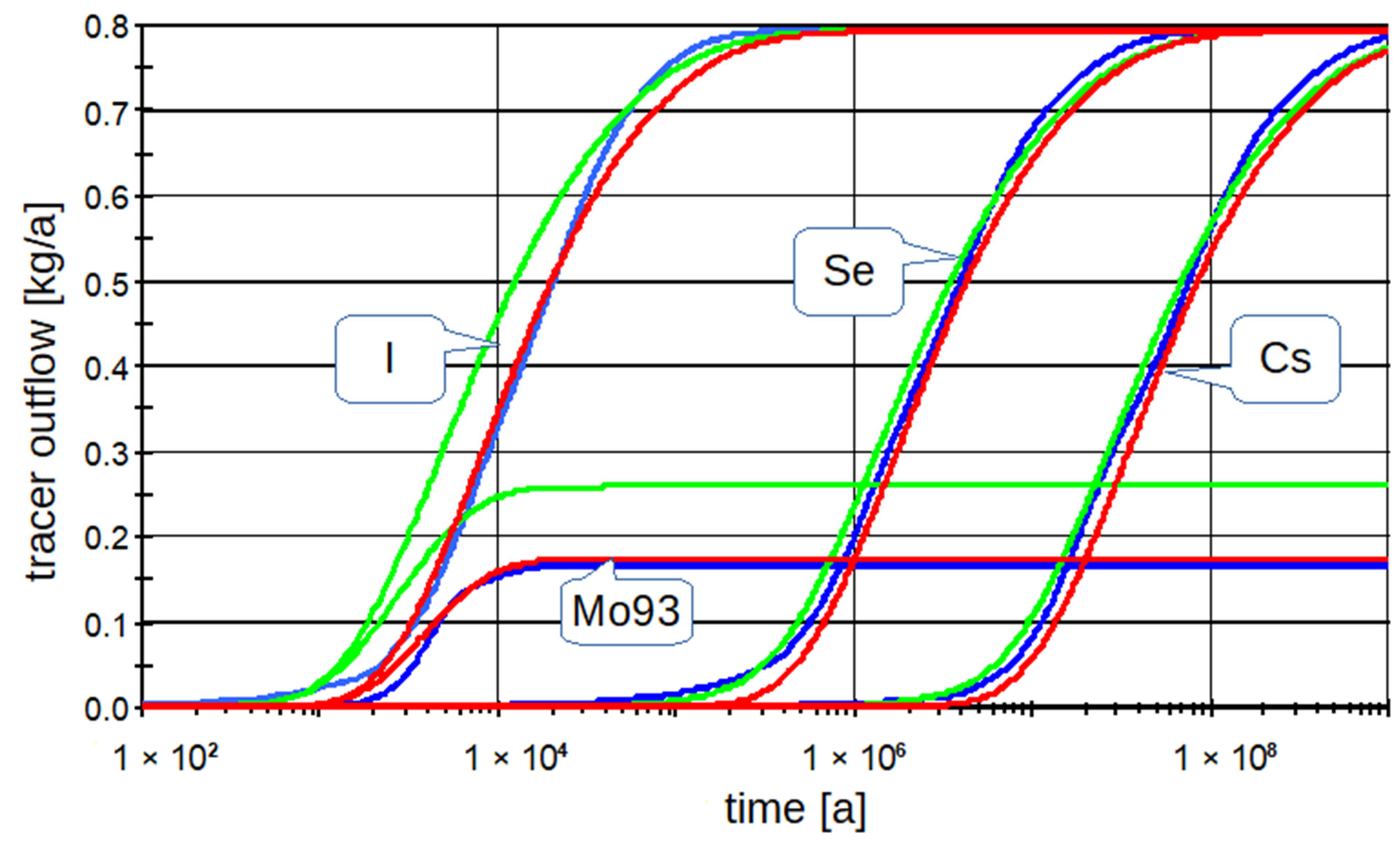
We chose three stable chemical elements as tracers: non-sorbing, I, medium-sorbing, Se, highly sorbing, Cs, and one non-sorbing radioactive nuclide, ⁹³Mo, with a half-life of 4000 a. Linear sorption was considered in the 3D model and the LPM (Kd concept), the K_d values were 0.0005 m³/kg for Se and 0.01 m³/kg for Cs. The source concentration was set (as fictitious) to 0.001 kg/m³, the same for all tracers, constant in time—to determine the transport pathway parameters, not for a real temporal evaluation in the safety assessment. Elements I, Se, and Cs were selected as inactive tracers, primarily to demonstrate the effects of their different sorption coefficients. The ⁹³Mo was selected as an active non-sorbing tracer because its half-life is of a similar order of magnitude as the transport time. Nuclides with higher half-lives may appear stable on this time scale, and nuclides with shorter half-lives do not reach the interface with the biosphere at all.

3. LPM Parameter Calculation

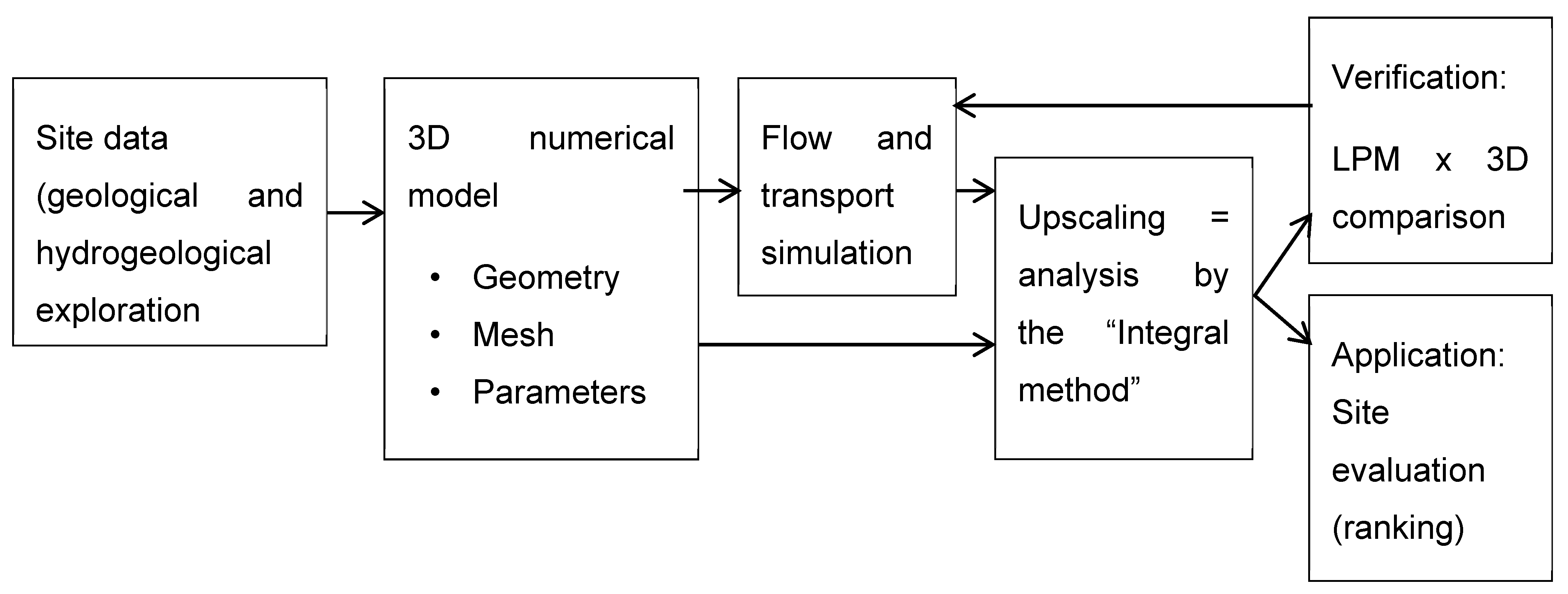
A conceptual scheme used to obtain the SA model and its parameters (Figure 4) is similar to what is found in other literature (e.g., [4,5]) and corresponds to the workflow in this paper. The suggested method provides a unique way to determine the parameters, which uses the results of the synthetic 3D transport model run and its initial geometric data (model configuration).

3.1. Concept of the Procedure

The purpose of the algorithm is to derive input parameters to the LPM (a fictitious transport path), which, at the same time, have roles in the safety characteristics (“indicators”). Such data are primarily (see also Figure 1):

• Inflow (i.e., groundwater flow from the storage area to the geosphere).
• Length (i.e., the distance traveled by groundwater from the storage area to the geosphere/biosphere interfaces).
• Flow time (i.e., the time taken for groundwater to travel the distance from the storage area to the interface with the biosphere).
• Dilution (the outflow/inflow ratio).

  ○

  Alternatively, outflow can be considered instead (the flow rate of contaminated groundwater from the geosphere to the biosphere).

We also consider other parameters determining the LPM (that can eventually contribute to the selection of the site or the safety assessment):

• Volume of the transport path.
• Data on the porosity of the transport path (minimum, average, maximum).
• Flow areas:

  ○

  Outflow area of the source, i.e., an area where the contaminant outflow from the storage space into the “geosphere” is present—geosphere inflow area.

  ○

  Total contaminated outflow area (from the geosphere to the biosphere).

• Breakthrough curves of selected tracers, i.e., the time courses of concentrations at the effluent into the biosphere, which are responses to unit jumps of concentrations at the source at time zero. These curves provide the data needed to determine the flow time.
• The same list of data for individual river basins (parts of the model).

We should note that “in” and “out” above are related to the “geosphere” as the studied system, if not stated otherwise.

These characteristics have their counterparts in the input of the LPM example, the “Pipe pathway” component of GoldSim software, representing the advective–diffusive transport with retention and dilution, with uniform parameters along the path. The relevant inputs, in this case, are: length, cross-section area, longitudinal dispersivity, the porosity of the infill medium, inflow, and outflow (six degrees of freedom, eventually characterized by seven parameters, including the travel time, dependent on the relation (6) below).

In the next two subsections, the calculations of the transport path (generic conceptual LPM) parameters from the 3D flow and transport model are explained. Later, the transformation into the pipe input parameter (particular LPM representation) is presented as part of the evaluation of the results in Section 5.

3.2. Lumped Parameters Calculation

The main set of parameters was derived from geometric characteristics of the discretization mesh, together with results of the flow and transport calculation with the step input of the tracer that was run until the steady state. The processing was mostly based on searching in the mesh, taking into account individual element data, such as volume, porosity, side area, the list of neighbors, calculated fluxes across element sides, and concentrations in the elements and at the sides. Technical details and pseudo-code expressions are provided in Document S2.

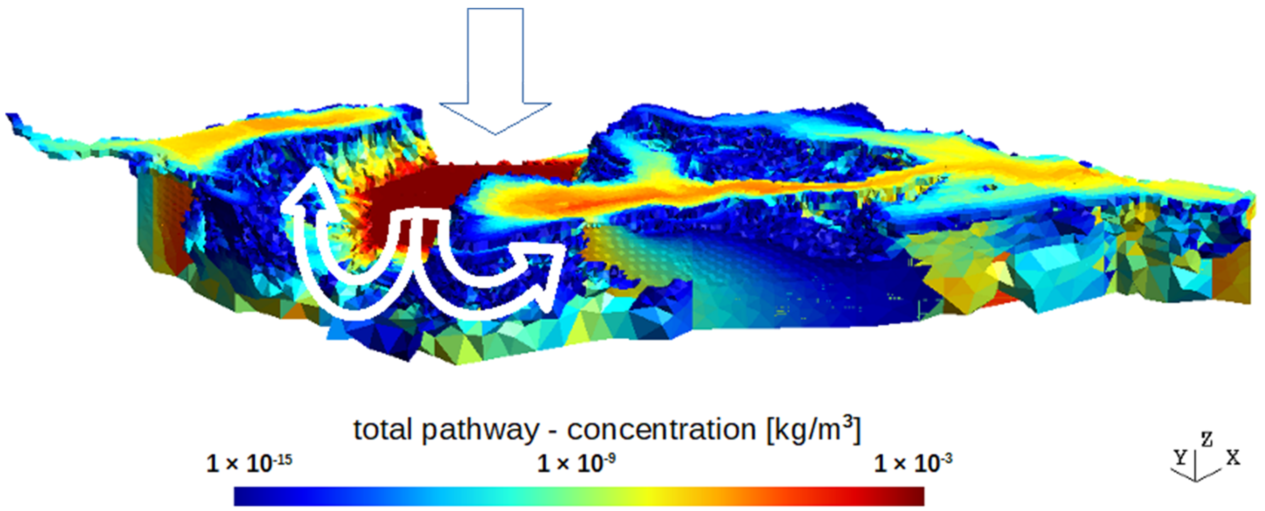
For the definitions of the volumes and areas reached by the contaminant (tracer), some threshold (“tolerance”) was necessary to be defined. For the volume, it was applied iteratively: the “next” element was contaminated if the ratio of flux from the current one to the next—to the total flux through the current element—was larger than the tolerance (a choice of 10⁻⁸ is used). For the outflow area, the tolerance was based on the ratio of the flux through the assigned “contaminated” area to the total flux out of the model. A value of 0.99999 was used for this case. The example of the tracer-accessed volume visualization is presented in Figure 3. We chose a contaminant outflow fraction of 0.99999 (99.999%); this choice was to limit the effect of the excessive dilution of the total flux. This number was a matter for the evaluator/evaluation team performing the safety analysis. It was possible to choose, e.g., 0.5 (50%), or to exclude flows with such low concentrations that the substance would not be present at all; that is, those where the concentration was lower than would correspond to the presence of at least one atom/molecule.

Here, the main parameters, procedures, and related conditions and assumptions are summarized:

• “Geosphere” inflow area $S_G^{in}$. Considering the repository volume is a part of the model domain, the interface repository/geosphere is supposed to be defined in the model input. The area is composed of the element sides between the repository subdomain and the geosphere subdomain with water flux in the respective direction. The procedure could be affected by the backflow described in Section 2. A compensation factor of the ratio between the total tracer outflow from the model (asymptotic in time) and the total tracer outflow from the repository (including the backflow), is used for correction.
• Water inflow into the “geosphere” $Q_G^{in}$ —calculated as a sum of fluxes through the respective element sides, considering an eventual correction for the backflow.
• Length of the transport pathway $L$. It is calculated by backtracking the tracer in the mesh. Starting from each outflow contaminated element, a neighbor element with the highest tracer flux is considered upstream in the path, and the distance of the gravity center is added to the length. Then, the average of all paths is made and weighted by fluxes in the respective outflow elements.
• Contaminated outflow area $S_B^{out}$—the sum of element sides based on the above threshold choice.
• Outflow rate of contaminated water $Q_B^{out}$—the sum of the fluxes through the “contaminated outflow area”.
• Volume $V$, porosity $\eta$ of the “path”—the sum of element volumes except the backflow cases, minimum ${\eta }_{min}$ and maximum ${\eta }_{max}$ values along the path.
• The dilution factor is postprocessed as the ratio of the outflow to the inflow values above.

3.3. Processing of Dirac Pulse Model Results

The second part of the parameter set is based on the processing of the breakthrough curve and the time evolution of the average concentration across the outflow area. The representative tracer travel time between input (repository) and output (biosphere) can be represented by the mean transit time, the first moment of the breakthrough curve, and a response to the Dirac tracer input pulse. From the outflow tracer evolution c(t), the meantime T is derived as

$$\begin{array}{c}T=\frac{{\displaystyle \int }c\left(t\right)·t·dt}{{\displaystyle \int }c\left(t\right)·dt}\end{array}$$

(1)

For the cases of sorbing tracers, the time variable was rescaled by means of the retardation factor before the application of the formula (2):

$$\begin{array}{c}{t}_{t,i}^{\prime }=\frac{t_t}{R_i}\end{array}$$

(2)

where i is the tracer index, R_i is the tracer retardation factor of tracer i, [-], t is the time step index, t′_t,i is the transformed time in step t, for time series tracer i, [T], t_t is the time in step t, [T]

The dispersion can be related to the second moment of the breakthrough curve c(t)—the variance σ² [T²] is calculated as

$$\begin{array}{c}{\sigma }^2=\frac{{\displaystyle \int }c\left(t\right)·{\left(t-T\right)}^2·dt}{{\displaystyle \int }c\left(t\right)·dt}\end{array}$$

(3)

and consequently, the longitudinal dispersivity d [L]

$$\begin{array}{c}d=\frac{D}{v}=\frac{\frac{{\sigma }^2·v^2}{2·T}}{v}=\frac{{\sigma }^2·L}{2·T^2}\end{array}$$

(4)

where D is the hydrodynamic dispersion coefficient, [L²·T⁻¹], T is the mean flow time, [T], L is the total length of the transport pathway, [L], v is the mean flow velocity, [L·T⁻¹].

4. Example Site Ordering

For an example of the evaluation and selection of a suitable location, we selected 11 parameters (in general, other sets are possible depending on the opinion of an evaluator):

• Inflow, i.e., the flow of groundwater from the repository space into the “geosphere”.
• Dilution of the outflow element with the maximum tracer concentration.
• Dilution of the outflow element with the maximum tracer flux.
• Mean dilution on the outflow elements in the “contaminated outflow area” (0.99999 shares of the total tracer flux).
• Flow time to the outflow element with the maximum concentration.
• Flow time to the outflow element with the maximum tracer flux.
• Mean flow of the outflow elements in the “contaminated outflow area”.
• Flow length to the outflow element with maximum tracer concentration.
• Flow length to the outflow element with the maximum flux of the tracer.
• Minimum flow length over all elements with a tracer flux, i.e., included in the “contaminated outflow area”.
• Mean flow length over the outflow elements in the “contaminated outflow area”.

These are directly given by the values explained above as results of the 3D model upscaling—the integral method. The list represents four quantities that have three variants of values depending on the choice of a single outflow element in the numerical discretization of the 3D model.

For indicator 1 (inflow into the geosphere), it is true that the lower it is, the more suitable the site is. For all other selected indicators, the higher they are, the more suitable the site. For each indicator, the ordering was determined for the tested sites according to suitability, i.e., the lowest flow had a value of 1, the second lowest had a value of 2, etc. For other indicators, it was reversed, so the highest value had an order of 1, the second highest had an order of 2, etc. Each indicator was multiplied by its weight, and then the sum of all indicators for each site was performed. The lower the sum, the more suitable the site.

Due to the fact that the selected indicators may have different importance, we chose two weight variants for demonstration and testing:

Variant 1: all indicators have (the same) weight of 1.

Variant 2: the inflow has a weight of 10, the medium dilution has a weight of 5, and the remaining indicators have a weight of 1; this variant is based on experience from previous projects [3,20,21] and should be more relevant.

Table 1. Example of two variants (weight choice explained in the text) of the site evaluation, resulting in the order of suitability (selected indicators shown due to limited space: 1,2,4,5,7,8,10,11).

Id	Inflow [m3/a]	Dilution [-]		Transport Time [a]		Pathway Length [m]			Evaluation
		Max Conc. Elm.	Mean of All Elms.	Max Conc. Elm.	Mean of All Elms.	Max Conc. Elm.	Min. Length Elm.	Mean of All Elms.	Variant 1		Variant 2
	(1)	(2)	(4)	(5)	(7)	(8)	(10)	(11)	Sum Indic.	Order	Sum Indic.	Order
l1	792	545	4205	11,589	25,478	1194	995	2597	37	3	63	1
l2	2116	15	531	2059	4725	1670	728	2674	69	6	164	8
l3	1637	589	4695	15,785	16,646	4647	1012	4414	25	1	65	2
l4	1648	69	2742	14,217	17,406	4323	650	3609	51	5	112	5
l5	1143	153	4162	49,095	20,071	7142	762	3813	29	2	68	3
l6	2085	44	1538	1105	13,096	855	663	2220	80	8	154	7
l7	4599	5	202	4087	4960	1604	723	1734	84	9	201	9
l8	2369	245	1416	5844	18,495	2490	1013	3971	46	4	142	6
l9	729	69	914	11,438	14,788	740	491	1381	74	7	111	4

shows the values of the selected indicators for all nine tested sites (denoted as l1–l9, anonymously representing the Czech candidate sites) as well as the evaluations according to the selected variants. In this case, site l1 is the best (according to the more relevant variant 2) as well as site l3, which is based according to both evaluation variants. Site l9 is completely unsuitable; sites l6 and l2 also appear to be unsuitable.

However, this assessment should only be taken as an example, the actual site selection must be made by a team of experts, taking into account other indicators and circumstances that cannot be included in these calculations.

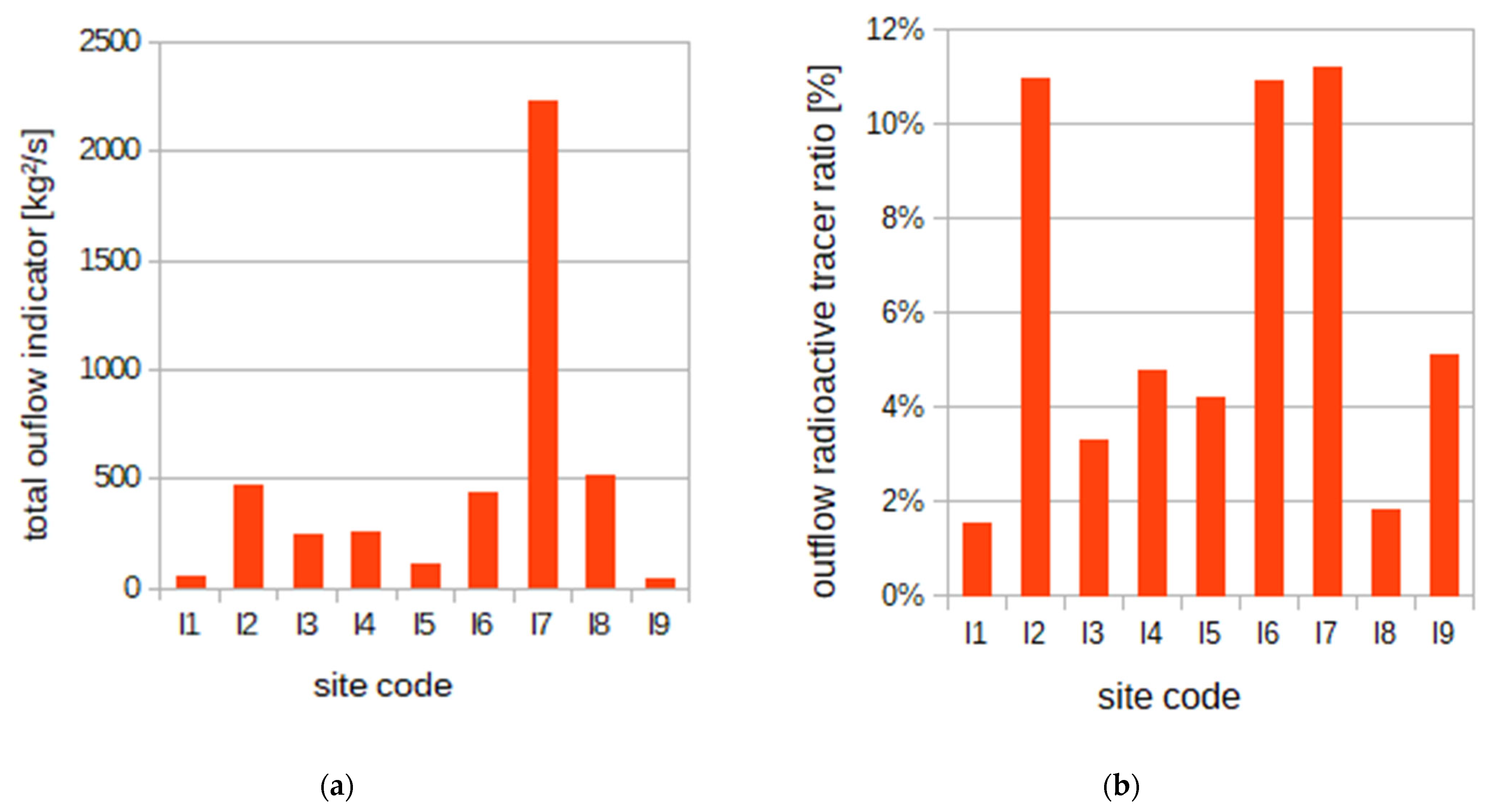
Additionally, the evaluation of the “total contaminant outflow” (the integral of the mass flux over time and the sum over all tracers, denominator in Equation (6)), as a single indicator, is presented in Figure 5a. It can be said that the lower this indicator, the more suitable the location. Figure 5b shows a more focused view on the indicator—a non-adsorbing radioactive tracer as (potentially) the most relevant representative for safety.

5. Comparison of LPM and the 3D Model

To demonstrate how efficient the integral method is to estimate the LPM parameters and how well the resulting LPM represents the “real” flow and transport process, both kinds of models are compared in this section. The example definition of the lumped parameter model can be taken according to the “Pipe pathway” compartment in the GoldSim software (the listed parameters are in Section 3.1).

5.1. Evaluation and Optimization Procedure

To compare the two models between each other, a suitable quantity of the model output and a fit criterion representing the difference (allowing optimization) needed to be defined. The temporal evolution of the contaminant outflow was used as the compared quantity (the integral over the time and sum over all tracers was used as the “total contaminant outflow”, one of the indicators for assessing the quality of sites (Section 4).

The sum of the integrals of the square of the difference (L2 norm), with normalization to the total contaminant outflow of the 3D model, was used as the optimization criterion:

$$\begin{array}{c}rel\_crit=\frac{{{\displaystyle \sum }}_j\left({{\displaystyle \int }}_{t=0}^T{\left(f{l}_{3D,j}\left(t\right)-f{l}_{LP,j}\left(t\right)\right)}^{2}dt\right)}{{{\displaystyle \sum }}_j\left({{\displaystyle \int }}_{t=0}^T{\left(f{l}_{3D,j}\left(t\right)\right)}^{2}dt\right)}\end{array}$$

(5)

where fl_3D,j is the tracer j outflow according to the 3D model [M·T⁻¹] fl_LP,j is the tracer j outflow according to LPM [M·T⁻¹], j is the tracer index, t is the time [T], T is the simulation time [T]. The normalization (the denominator in the formula) helps to obtain comparable results of the model fit for different evaluated sites or model geometries.

For the evaluation in this section, we considered three model results:

• The 3D model (Flow123d results as the example).
• LPM with the parameters calculated by the integral method (Section 3).
• LPM with optimized parameters based on the defined criterion (GoldSim processed).

Optimization confirms how good the “prediction” is, i.e., checks the relevance of the LPM parameters calculated from integral processing of the 3D model inputs and results. If the optimized LPM, i.e., with parameters minimizing the criterion (5), provides a significantly better fit, it indicates a not-so-efficient method for the upscaling (integral method), and vice versa.

As presented below, one sample site was evaluated in detail with all of the listed parameter values and with the breakthrough curves of the three compared models. Then all sites are presented more coarsely with selected evaluation data. Additionally, more complex LPMs were tested, with two or three pipe components of independent data, representing more precisely the transition of the flow field from the repository scale to the site scale.

5.2. Example of One Sample Site Processing

For an example of using one “Pipe” component, we used data obtained by postprocessing a non-sorbing tracer (I). All used data are in

Table 2. Parameters obtained by the postprocessing and by the optimization used to set one “Pipe” component. The last row represents the evaluation of fit between the LPM and the 3D model.

LPM Parameter	Units	Postprocessing	Optimized
Flow length	m	2597
Cross section	km2	3724	5516
Longitudinal dispersivity	m	4707	5161
Porosity of the filling medium	%	0.8774
Inflow	m3/a	791.9
Outflow	m3/a	3,329,904
Dilution	-	4205
Transport time	a	25,478	37,741
Value of rel. opt. criterion (5)	%	0.2	0.007

. Besides the directly available data ($Q_B^{out}$, $Q_G^{in}$, L, η, d), the cross section S [L²] of the “Pipe” component is calculated by Equation (6) from other evaluated data

$$\begin{array}{c}S=\frac{T·Q}{L·\eta }\end{array}$$

(6)

where L is the length [L], Q is the flow rate [L³·T⁻¹] (i.e., outflow $Q_B^{out}$ introduced above), T is the travel time [T], and η is the porosity of the filling [-]. It means that the derived generic transport path parameters overdetermine the pipe component parameters—the evaluated areas $S_G^{in}$ and $S_B^{out}$ were not used at all to keep the model consistent with the travel time according to (6). Additional parameters not necessary for the LPM calculation are included in Document S3.

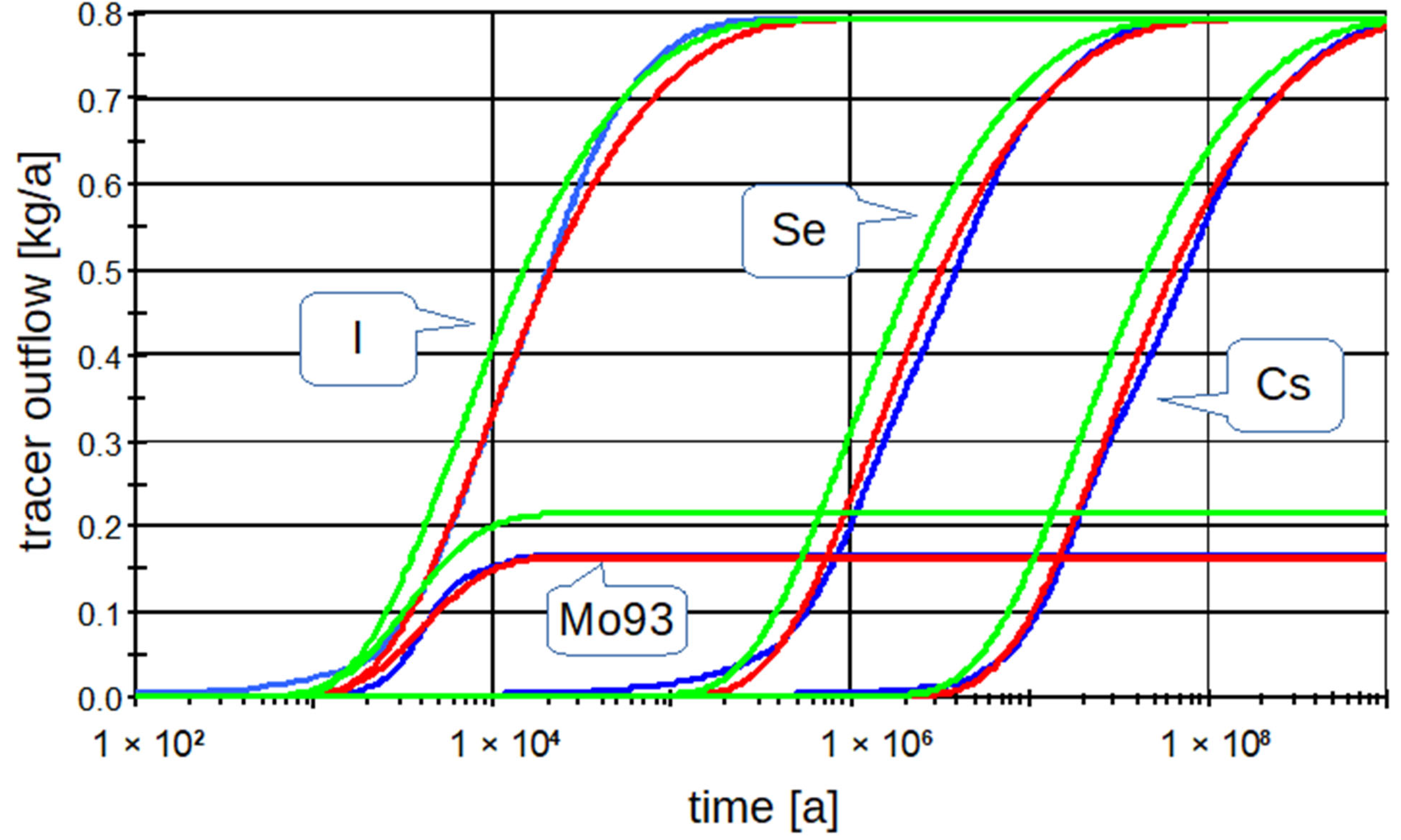
The resulting values of the optimized parameters, including the values of the optimization criterion, are listed in Table 2. The resulting breakthrough curves of the tracers are shown in Figure 6. It can be seen that even a single optimized component “Pipe” shows results almost identical to the results of the whole 3D model. However, in this case, it should be noted that the defined transport path has an unrealistically large cross-section of the order of several thousands of km² (that is about 1000 times larger than the model area). This is due to the fact that the entire “Pipe” component comprises the flow rate equal to the “outflow” (flow of groundwater from the geosphere to the biosphere), which is orders of magnitude larger than a realistic inflow. To comply with the transport time, Equation (6) leads to a large cross-section. This problem is resolved in Section 5.4 and Section 5.5.

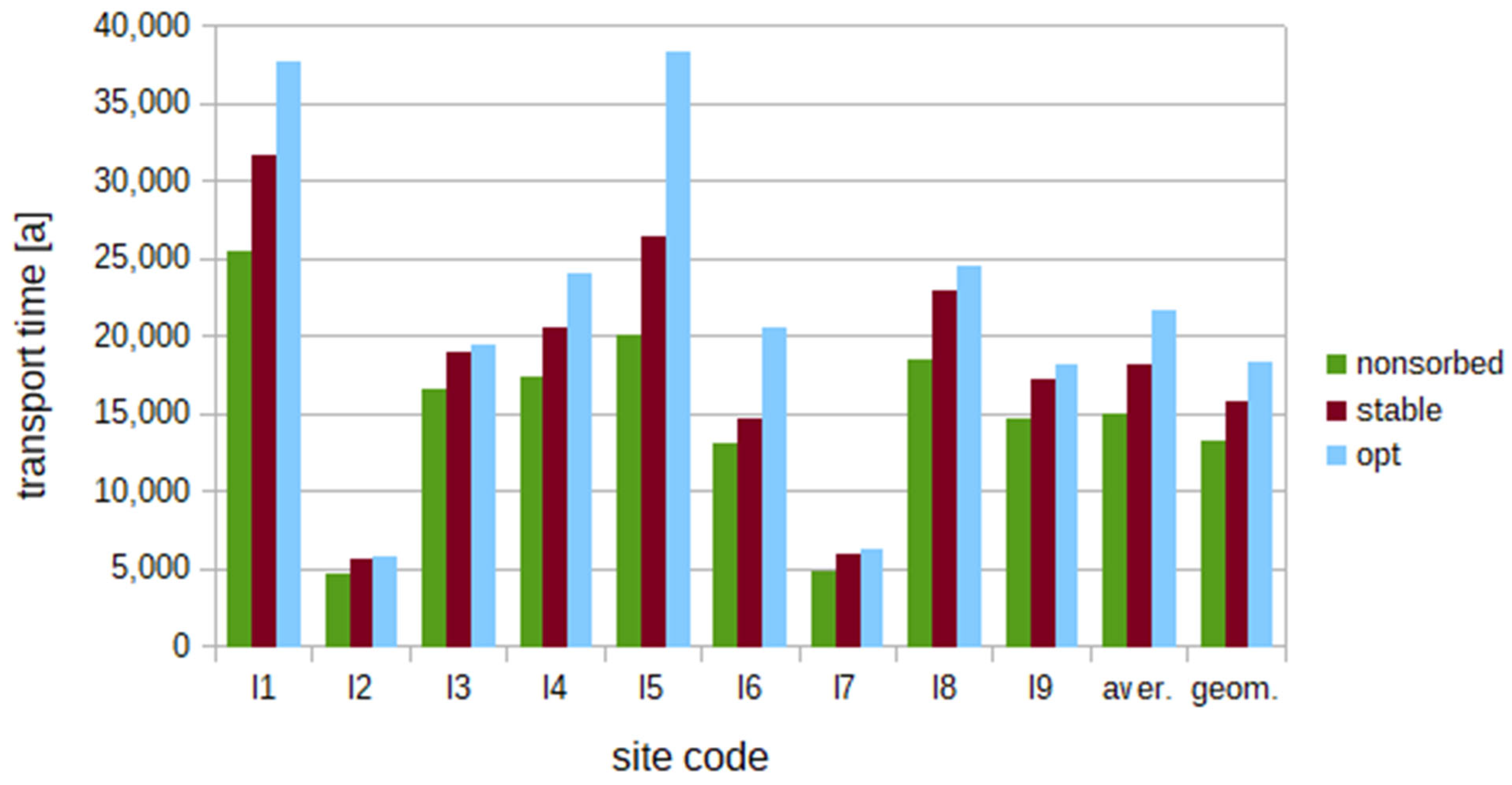
5.3. Results of the Single Pipe Model for All Sites

The parameters for the “Pipe” were determined for both the non-sorbing tracer (iodine) and the average of the three stable tracers (iodine, selenium, and cesium, referred to as “stable” in Figure 7). Furthermore, optimization was performed using GoldSim for the “transport time” and “dispersivity” parameters (referred to as “opt” in the legend).

The results are shown in

Table 3. Longitudinal dispersivities (m) for test sites postprocessed from the non-sorbing tracer, from the average of the stable tracers (“stable”) and the optimized values. There are also (arithmetic) and geometric averages over all sites.

Site	l1	l2	l3	l4	l5	l6	l7	l8	l9	Aver.	Geom. Aver.
Non-sorb.	4.707	6.079	12.597	6.902	7.015	20.273	6.955	7.904	6.223	8.739	7.909
Stable	5.488	7.065	13.391	8.788	8.764	20.862	9.150	9.719	7.162	10.043	9.322
Optimized	5.162	5.374	7.288	12.012	18.973	25.219	4.311	5.174	3.573	9.676	7.677

and

Table 4. Values of the relative criteria (%) for test sites for models derived from the non-sorbing tracer data, from the average of the stable tracers (“stable”), and for the optimized model. There are also (arithmetic) and geometric averages over all sites.

Site	l1	l2	l3	l4	l5	l6	l7	l8	l9	Aver.	Geom. Aver.
Non-sorb.	0.208	0.095	0.488	0.038	0.128	0.074	0.25	0.57	0.555	0.27	0.19
Stable	0.086	0.042	0.332	0.026	0.148	0.035	0.241	0.425	0.477	0.2	0.13
Optimized	0.0068	0.0025	0.0032	0.0137	0.0372	0.0066	0.0007	0.0022	0.0015	0.008	0.004

, and Figure 7. The resulting transport times are slightly lower from the data of the non-sorbing tracer than according to the averages of all three stable tracers. With the help of optimization, the transport times are even higher.

The resulting dispersivities for the non-sorbing tracer are always slightly lower than the average value for all stable tracers, but the optimization, in contrast to the transport times, gives various cases of lower and higher values. It should be noted here that the dispersivities determined in this way are two to three times the length of the transport path, but the recommended value according to the GoldSim manual is 10% of the length.

The evaluation of the quality of the model of one “Pipe”, created in the GoldSim software environment, can be assessed using a relative criterion (5). These “error” values do not exceed 0.6% even for the “worst” estimates according to the non-sorbing tracer. For optimized parameters, the average error is 0.008%, see Table 4. Therefore, it can be said that the LPM can be set as described above so that it gives values that are sufficiently close to the results of the 3D model, and, if we use the optimized parameters, the difference is small compared to, e.g., numerical errors in the 3D model.

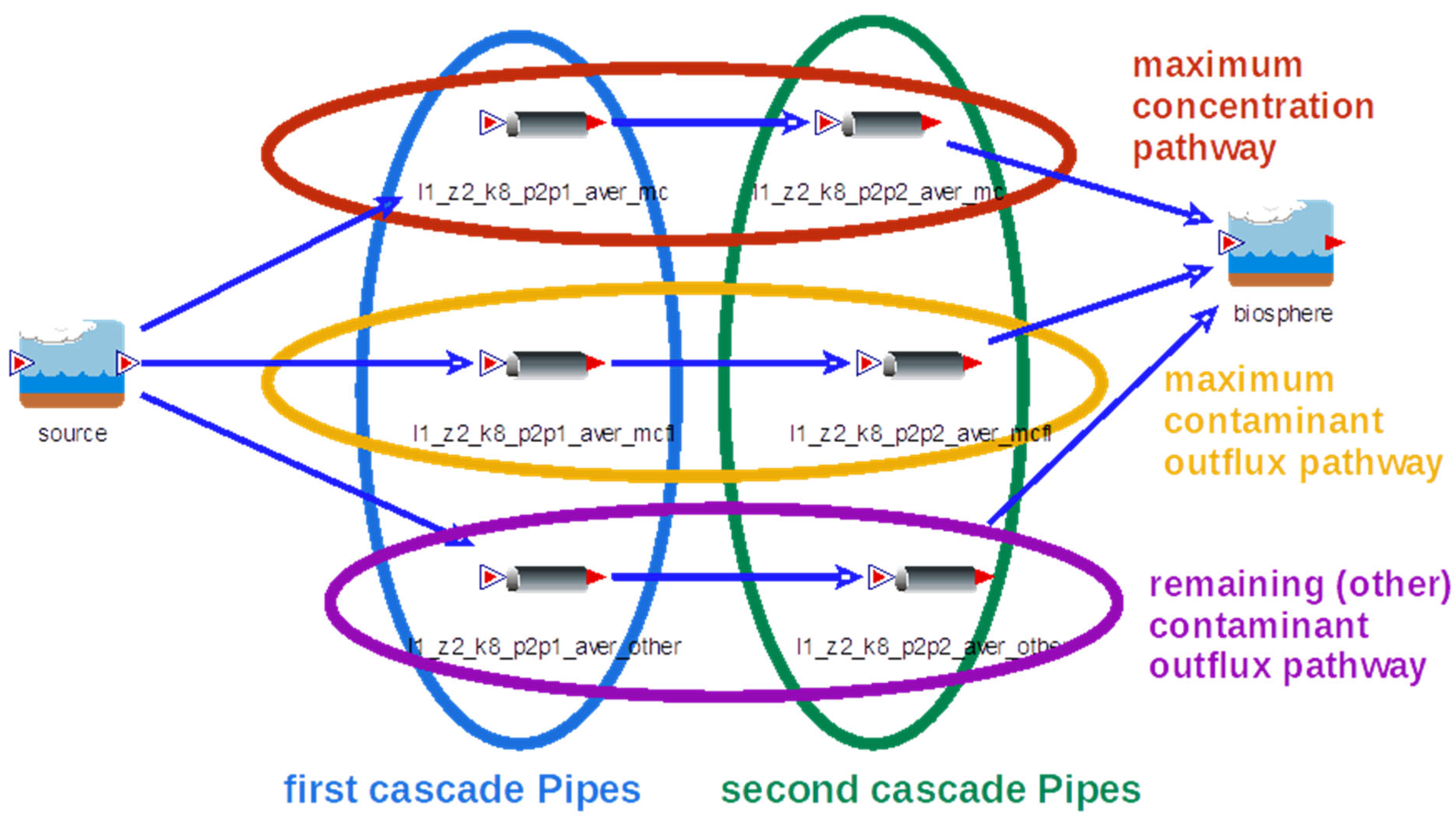
5.4. Results of Two Cascade Pipes Variant

To obtain a more physically realistic model, we considered the case with more degrees of freedom: the transport path was divided into two parts serially, represented by two model pipes. The mathematical formulation and derivation are shown in Document S3. Including the travel time—seven parameters for each pipe needed to be set from eight evaluated parameters in Section 3. The first pipe had the same inflow rate and outflow rate, equal to “inflow to the geosphere”, $Q_G^{in}$; the second pipe had the inflow rate equal to the first pipe’s outflow and the outflow rate was equal to the “outflow rate of contaminated water”,$Q_B^{out}$, i.e., it included the dilution. Cross sections were also set in the first pipe as the geosphere inflow area, $S_G^{in}$, and in the second as the contaminated outflow area, $S_B^{out}$. The total length and total transport time were maintained, constituting two additional constraints, as well as another two given by “continuity” Equation (6) for each pipe individually. The dispersivity was the same for both pipes.

To determine the two independent porosity values, one degree of freedom would remain if only the total (average) porosity of the path was available. We tried more variants to resolve it. The first variant assigned the minimum porosity of the transport path to the first pipe, and the maximum porosity to the second pipe (“min–max”, Sections S2.1 of S3). Other variants were set so that (1) the first pipe had the minimum porosity, and the second had a porosity such that the total mean porosity agreed with the total mean porosity of the transport path determined by the postprocessing (“min–aver”, Sections S2.2 of S3) and (2) analogically the average maximum case (Sections S2.3 of S3). In such a way, the first pipe was interpreted as a part through the matrix or undisturbed rock with small fractures (low porosity, small flow rate, low velocity) and the second part as a permeable zone (high porosity, large flow rate, large velocity).

For site l1, a comparison is presented in

Table 5. Postprocessed and optimized parameters of both the pipes in the cascade configuration and their total values (sum or average, respectively), for site l1. The variant “min–max” for the porosity and the optimization option with two independent dispersivities are shown.

Parameter	Units	First Pipe		Second Pipe		Total
		Postproc.	Optimized	Postproc.	Optimized	Postproc.	Optimized
Flow length	m	2129	1987	468.0	609.3	2597
Cross section	m2	2,390,830		514,868		Not defined
Longitudinal dispersivity	m	4707	4123	4707	3650	4707	4012
Porosity of the filling medium	%	0.3964	0.6051	5.0		0.6045	0.8774
Inflow	m3/a	791.9		791.9		791.9
Outflow	m3/a	791.9		3,329,904		3,329,904
Dilution	-	1		4205		4205
Transport time	a	25,474	36,304	3.62	4.71	25,478	36,309
Opt. criterion	kg2/s					0.1969	0.02919
Rel. criterion	%					0.35	0.051

for the min–max variant of porosity and optimization of the flow time and the dispersivities for each pipe separately (“basic”). Other variants of optimized parameter sets were (1) flow time and dispersivity common for the pipes, and (2) the basic case plus the flow rate between the two pipes as a new degree of freedom.

It can be said that the variant with the total mean porosity according to the non-sorbing tracer had a slightly worse criterion than the variant with the min–max porosities. Basic optimization, where the dispersivities were optimized for both cascade pipes independently, did not have a significantly better result than (1) when the optimized dispersivity was the same for both pipes.

The worsening of fit compared to the single pipe model with fewer parameters was an effect of adding new constraints that ensured both pipes had more realistic parameters.

5.5. Results of Three Cascade Pipes Variant

In addition to the model generalization into the two pipes, we created a model for the three cascade pipe components so that even more characteristics of the transport path could agree to realistic values, i.e., the flow length, the travel time, the total middle porosity, and the total volume. The relationship for the calculation of the cross section of the middle “Pipe” was based on the assumption that in the first approximation, the transport path had a shape of two consecutive truncated cones with a common base.

The constraint equations (Document S3) composed a system of three algebraic equations for three unknown lengths of the individual pipe. Thus, the solution of these equations can be used for optimization using GoldSim software.

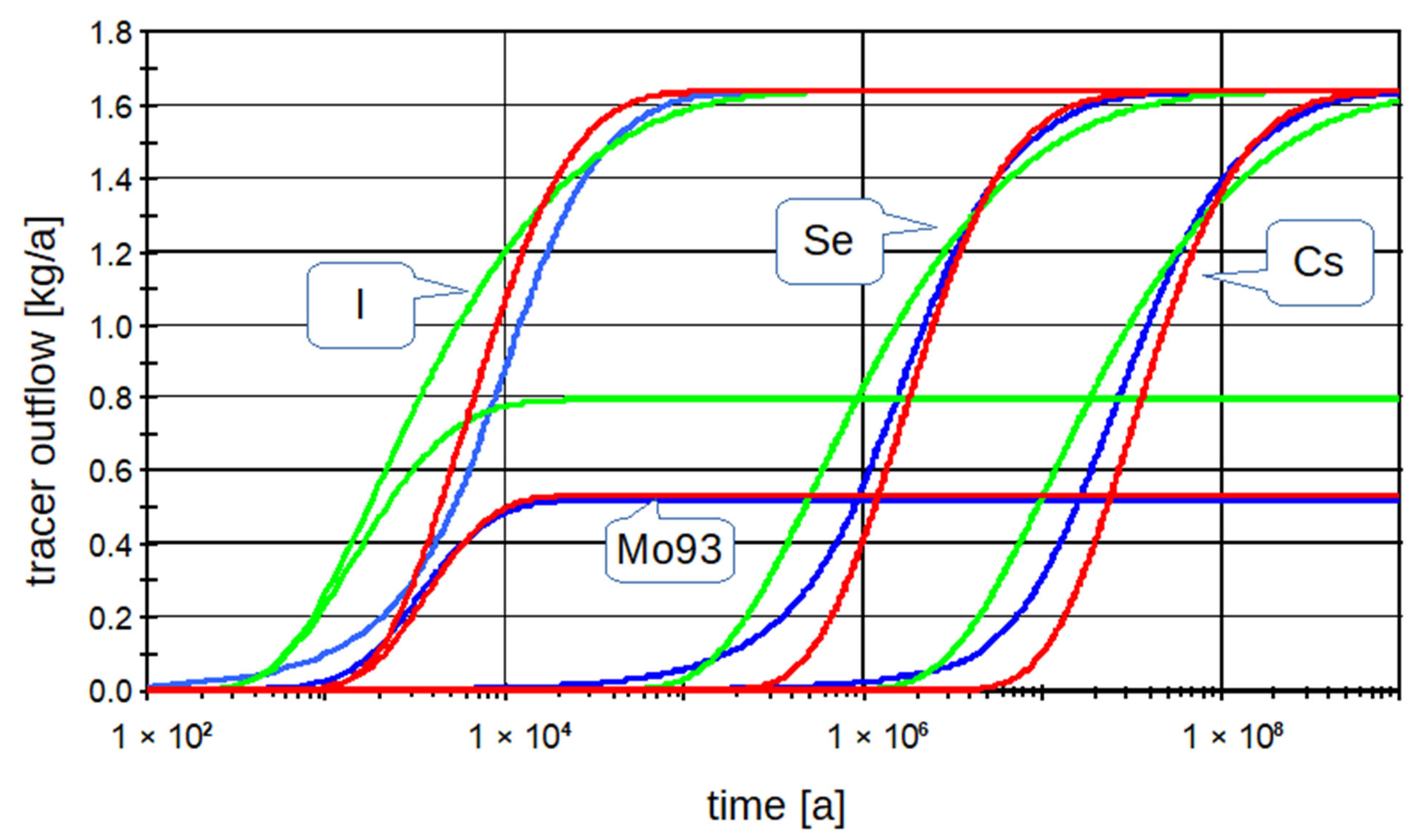
For example results with the three cascade pipes, we chose site l3. It should be noted that this procedure resulted in a negative length of one of the parts (usually the second or the third) in about half of the cases and, therefore, could not be used for such sites (not in the case of l3). The resulting comparison of breakthrough curves is shown in Figure 8.

5.6. Results of Parallel Pipe Structures

For safety analyses, it was necessary to find the place or area with the highest contamination. If the results of the models showed divisions of the flow of activity into several streams, two or more river basins (catchments) may have been affected, with different concentrations or contaminant fluxes. Therefore, we divided the flow into several parts according to the requirements of SA. Such a division may be, for example, according to the river basin, where each contaminated river basin may have different biospheres; thus, it was necessary to have a different biosphere model for each river basin, or at least different biosphere parameters, see Figure 9.

In an example for site l1, parallel paths were introduced, based on different criteria at the geosphere outflow, instead of physically different outflow areas (more catchments). We found the outflow element with the highest concentration and the element with the highest contaminant outflow. In general, these elements may be the same, but in our case, they were different. So, we had two transport paths, one for the maximum contaminant concentration and the second for the maximum contaminant outflow. The third path was differential, representing the remaining flow. Thus, the sum of these three transport paths represents the total flow. The resulting breakthrough curves for this case are presented in Figure 10. The fit is comparable to (or better than) the variants above.

6. Conclusions and Outlook

In this work, possibilities to build LPMs (with their advantages of simplicity and computational efficiencies for typically repeated runs within stochastic computations of safety assessments) supported by 3D hydrogeological model data (with as much as possible disposal site knowledge) were generalized and extended.

Although it can seem that the complexity of the 3D heterogeneous transport could not be captured by one or a few “pipes”, the presented numerical examples justified such an approach, including its use in the past with generic parameters. The new message from the comparison of the upscaled and optimized LPM is that the parameters to define such an LPM can be defined by a rigorous procedure from the real hydrogeological configuration projected into the 3D model to a larger extent than with particle tracking approaches. Such a comparison was not available for lumped parameters obtained for individual pathways.

This paper demonstrated a two-fold use of the results: support for the comparison and selection of the candidate sites and the setting of the LPM available for effective calculation in the SA.

The method provides certain freedom for the authors of the SA to fit a particular purpose of the derived LPM. Through the ratio of the total mass accounted to define the tracer-accessed volume (Section 3.2), the initial idea of the integral pathway comprising the whole flow field was generalized to specific pathways capturing, e.g., a case of maximum concentration considered as a part of the SA (Section 5.6).

It was found that, while a single pipe compartment provides a good model fit, it is convenient to split the model into two or three “cascade” pipes, which actually means an increase in the model parameters. As such models need to be accompanied by more constraints, it does not necessarily improve the fit to the 3D model. The two-pipe variant leads to a slightly worse fit criterion than the single pipe, but it provides a significantly better physical meaning of the parameters and improves the reality abstraction in the LPM, thanks to the added constraints.

Therefore, the integral method gives realistic results, which are needed especially for safety calculations and analyses of deep geological repositories of high-level waste. It should be noted that the presented models and calculations are not actual safety assessment calculations. Tracers used in the transport model possess only part of the features of the corresponding radionuclides escaping from the repository and are used as intermediate tools to upscale the model transport properties. The resulting LPMs from the presented method can (afterward) be supplied with input data of the realistic decay chains, sorption coefficients, and generic temporal variability of the model data.

Further development and testing are possible, e.g., testing other types of signals (e.g., unit pulse). The method could be tried on a model in which the main transport path will be a fracture or a fault zone. Finally, the analysis and adjustment of the procedure for the three cascade “Pipes” could be useful, so that they always give real values.