Abstract
Energy Efficient Building (EEB) design decisions that have traditionally been made in the later stages of the design process now often need to be made as early as the feasibility analysis stage. However, at this very early stage, the design frame does not yet provide sufficient details for accurate simulations to be run. In addition, even if the decision-makers consider an exhaustive list of options, the selected design may not be optimal, or carefully considered decisions may later need to be rolled back. At this stage, design exploration is much more important than evaluating the performance of alternatives, thus a more transparent and interpretable design support model is more advantageous for design decision-making. In the present study, we develop an EEB design decision-support model constructed by a transparent meta-model algorithm of simulations that provides reasonable accuracy, whereas most of the literature used opaque algorithms. The conditional inference tree (CIT) algorithm exhibits superior interpretability and reasonable classification accuracy in estimating performance, when compared to other decision trees (classification and regression tree, random forest, and conditional inference forest) and clustering (hierarchical clustering, k-means, self-organizing map, and Gaussian mixture model) algorithms.
1. Introduction
The main goal of the design of Energy Efficient Buildings (EEBs) is to reduce both the energy demand and energy use. To achieve this, designers consider a number of variables during each of the design stages and continuously evaluate the effects of their combination on the energy performance of the building. In particular, design variables that are set during the feasibility analysis stage, such as volumetry and orientation, not only play a critical role in reducing the building energy demand and minimizing the capacity of the heating, ventilation, air conditioning (HVAC) systems, but also greatly impact the costs of a construction project. Thereby these EEB features should be established, or at least considered, at the feasibility analysis stage, because incentives and the constraints associated with these features greatly influence the overall economic feasibility. Indeed, many previous studies on EEB design have indicated that great care should be taken to select design variables during the early design stages [1,2,3,4].
For sophisticated EEB projects, however, only highly experienced designers or consultants are likely to know exactly which design variables should be selected for a given budget and timeframe, what values should be set at each stage, and how each design variable interacts with others. It is because the accumulation of many small differences in the individual building physics and the energy system can lead to synergetic or dysergetic effects across the entire design, thereby making the selection of design variables and their values differ from legacy practices.
To quantitatively determine which design variables affect a specific measure of building energy performance, designers and engineers typically employ simulations to assess synergetic and dysergetic effects in case-specific designs. However, to appropriately use building simulations, expertise in building physics and system mechanics, design experience, long-term software training, and skills in how to use simulation tools are required. Thus, simulations may not be a useful support tool for design decisions for general building designers who are actually simulation consumers [5].
2. Relevant Practices and Studies in EEB Design Support
2.1. Sensitivity Analysis
Sensitivity analysis (SA) has been one of the most widely used general design decision support tools [6]. SA is able to suggest primary design variables in an intuitive and convenient manner by automating design variable selection and variable-specific range setting, and then executing numerous simulation runs in batch mode. However, although it may identify the design variables that are most sensitive to the context of the target building, SA does not designate values, thus values still need to be decided by the designer. Furthermore, all the design variables are assumed to be independent in SA. It is thus difficult for the designer to consider chain reactions between design variables when their values are initially set.
2.2. Design Optimization
Similar to SA, design optimization creates a problem space with a large number of design combinations that are applied to a base model for the target building [7,8]. Design optimization then searches for the most optimal solutions using a mathematical optimization algorithm that evaluates the objective function (e.g., the energy use) of each combination of design variables and their values. Unlike SA, design optimization provides both the design variables that are sensitive to the context of the target building and their values. Because the correlations between the design variables are identified by the algorithm, once a particular design is selected based on the preferences of the designer from among the Pareto solutions, the configuration of the design variables and their optimal values have already been set. Therefore, the designers do not need to worry about the selection of other design variables.
However, if the optimal design variables proposed by the optimizer are not selected by some reasons (e.g., if the client wants to replace the suggested variables and values with other preferences after initial setups), the problem space must be recreated, and another exhaustive search of this space must be conducted. As a result, the design progress may be delayed due to unexpected and/or human-generated uncertainties.
In addition, optimization is not transparent in terms of how the optimal solution is selected, thus users may doubt the selection process and question the credibility of the optimal solution. Indeed, knowledgeable designers and engineers want to know how machine-suggested optimal solutions are determined, because they are ultimately responsible for the selected design.
2.3. Meta-Model
Because both SA and optimization evaluate a number of instance simulation models, the computational time required to search for the most optimal solution can be prohibitive. For this reason, large problem spaces are often constructed in a cloud computing environment in advance and left on standby for when the designer is ready to make their selection. These online problem spaces are created by simulating the behavior of an analytical model using a meta-model [9,10,11]. Recent trends in the use of meta-models for EEB designs can be found in [12].
Technically, a meta-model is a data-driven model produced using machine-learning algorithms. Some of the most popular algorithms used for meta-models in architecture, engineering, and construction (AEC) are linear and multivariate regression [10,11,13,14,15,16], artificial neural networks (ANNs) [10,15,17,18,19], support vector machine (SVM) [9,20,21,22], Gaussian process models (GPMs) [10,14,23,24,25], and radial base functions (RBFs) [25,26,27,28]. Because machine-learning algorithms aim to predict and classify new observations based on trained criteria, they are usually employed to cover all the design variables for the target building and to include all possible ranges for each variable. From the perspective of a user, these machine-learning algorithms are computationally less intensive than analytical simulation models. Thus, the energy performance of the target building can be assessed in real time for almost all design cases even if the client changes the requirements arbitrarily, such as requesting that specific variables be adjusted or excluded all of a sudden. Overall, a meta-model offers a relatively exhaustive problem space, uses a systemic search mechanism, and produces quantitative solutions.
Whether a machine-learning algorithm produces an opaque or transparent model depends on whether the users can witness the branching process of the solution space. For example, a transparent model (e.g., a decision tree) discloses the intermediate branching and result selection process, whereas an opaque model (e.g., an ANN) does not reveal the development process but only provides the solution in the final stage. However, because opaque machine-learning models are known to be more accurate so far, most previous studies on the selection of design variables for EEBs have utilized meta-models with opaque machine-learning algorithms [29]. However, designers prefer transparent and interactive methods that allow for creativity and produce more diversity, because they can eventually lead to the most diverse design solutions [30] compared to black-box approaches such as optimization and opaque process.
3. Study Objectives
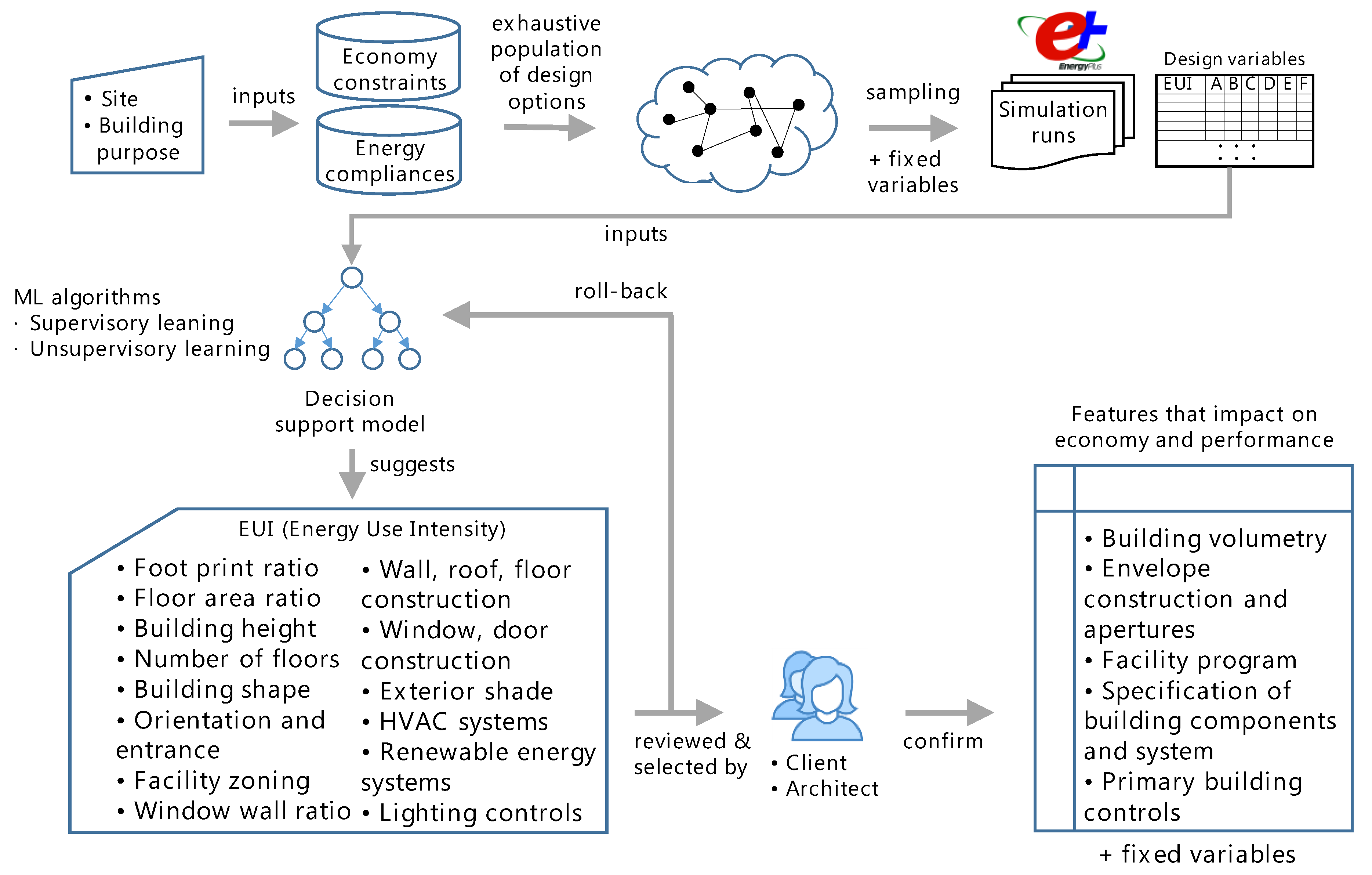
In practice, design decision support should consider irrational and unexpected settings and/or results in the early stages of the decision-making process. Accordingly, an EEB design decision-support model should have a robust structure and mechanisms that support trial and error in the design process. In this way, the decision model can visually provide designers with a variety of decision options (Figure 1) rather than simply presenting the optimal conditions; first the user inputs site and building purpose; then, exhaustive combinations of design options are drawn out of the economy constraint and energy compliance databases. Then energy performance of representative samples is evaluated by simulation. Eventually the option combination and its simulation result are built as a surrogate model. Once a user selects specific design variables and their values, the surrogate model can display the follow-up design variables. This would help stakeholders to intuitively select EEB design variables and values from among the displayed alternatives and help them to understand how these choices affect the economic and energy performance given the underlying associations between the variables.
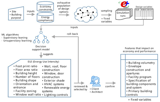
Figure 1.
The EEB design decision support system at feasibility analysis stage.
In summary, the functional requirements for EEB design decision support in the very early design stages are as follows:
- I.
- Users should be able to make prompt and informed decisions after fully recognizing and understanding the influence of the chosen design, the alternatives, their countermeasures, and if the chosen design turns out to be inappropriate.
- II.
- Although not all the design variables need to be exhaustively covered, a sufficiently reasonable number of energy-sensitive design variables that are suitable for the context of the site and the construction project should be presented.
- III.
- When a specific design is selected, the primary Energy Use Intensity (EUI) of that design should be predictable with reasonable accuracy, which indicates the energy associated with fuel production, transformation and distribution, and losses to provide building site energy such as electricity and municipal gas.
If a meta-model is built based on a reasonable number of simulations that sufficiently represent the design space, it will be able to meet these requirements for EEB design decision support. The additional technical requirements for machine-learning algorithms in meta-models for design decision support are as follows:
- I.
- The meta-model should have a transparent structure with different design paths for possible options when users (as stakeholders) select design variables and their values. As such, if the user desires to reassess the chosen design, they can retrace it to the break-even point and restart the selection process.
- II.
- The meta-model should be able to predict how the EUI will be affected by a change in design within a reasonable variance whenever the value for a design variable is revised by the stakeholders.
4. Clustering and Decision Tree Algorithms to Build a Transparent Meta-Model
Machine learning algorithms are divided into supervised and unsupervised learning algorithms. The supervised learning algorithm describes the relationship between the input and object variables, and quantitatively represents the model structure. The object variable is determined according to the purpose of the data analysis, which is normally selected by the domain expert. In supervised learning, once a model structure is set and the properties are updated by the collected training data, the training data are substituted with new data to classify the new observations and predict the response. Accordingly, the quality of training data determines the robustness and fidelity of the developed model. Typical supervised learning algorithms, except for the decision tree and some regression models, are black-box models, in which the relationships between the independent variables (input variables) and the relationships between the independent and dependent variables (input-output variables) are not directly visible.
In contrast with supervised learning, unsupervised learning does not set the data-mining target. Because the target variable is not set intentionally, the input and output variables are not separated but are considered variables of interest. Whereas the supervised learning is a backward analysis that continuously adjusts properties of the meta-model until the calculated output matches the measured output, unsupervised learning is a forward analysis that eventually discovers correlations and associations between variables and finally aims to uncover the structure of the meta-model until predefined criteria are met. Therefore, the prominent advantage of unsupervised learning is the ability to discover previously “unknown” knowledge, if any. For instance, clustering separates raw data into groups whose patterns are similar after analyzing the patterns of all variables, whereas the purpose of rule mining or motif discovery is to directly extract statistically significant rules and motifs. Prior clustering and dimension reduction can be performed as prescreening; PCA (Principal Component Analysis) combines variables linearly to configure new agency variables, whereas FA (Factor Analysis) linearly combines variables whose patterns are similar to differentiate the combined variables from other variables [31].
As the purpose of this study is to prepare a meta-model with a transparent structure that can visually represent the causality and relation between EEB design variables, unsupervised learning seems to be more appropriate for the purpose. However, some regression models or decision trees in supervised learning algorithms can also create a meta-model with a transparent structure.
The regression algorithm in supervised learning is a mathematical formula that expresses the effects of independent variables on the dependent variables by a number (i.e., a weight). The correlations between independent variables are also expressed in the same manner. However, if the number of independent variables (n) increases, the number of correlations also increases by n!, and if the number of variables has an n-dimension or larger relationship (e.g., polynomial regression), it cannot be expressed using a mathematical formula but must use a matrix. Thus, it is difficult for users to know the model structure intuitively.
In unsupervised learning, pattern detection algorithms, such as rule mining or the motif discovery algorithm, are advantageous to identify sequential orders when there are many transactions. For example, these algorithms are excellent performers that can discover a causal relationship between specific products using many product sale histories (e.g., correlation between diaper and beer sales) or can estimate operating sequences between plant systems and air-conditioning systems as a form of inference rules.
For the above reasons, and as summarized in Table 1, we investigated clustering algorithms from unsupervised learning and decision tree algorithms from supervised learning. Eventually the following specific clustering and decision tree algorithms are chosen for each group. It should be noted that random forest and conditional inference forest algorithms do not result in intuitively visible structures, although they are still transparent decision trees. These two forest algorithms were intended to compare accuracy among decision tree algorithms, namely, single tree vs. forest algorithm.

Table 1.
Comparison of transparent algorithms.
- Clustering: hierarchical clustering (HC), k-means, self-organizing maps (SOM), and Gaussian mixture model (GMM)
- Decision tree: classification and regression tree (CART), conditional inference tree (CIT), random forest (RF), and conditional inference forest (CIF)
4.1. Clustering Algorithms
Clustering gathers similar data whose behaviors or patterns are analogous. The similarity is determined by calculating the Euclidean distance between data or the maximum likelihood via the Expectation–Maximization algorithm (EM), which is one of the most practical methods for learning latent variable models in unsupervised learning [32].
4.1.1. Hierarchical Clustering (HC)
Hierarchical clustering is the most widely used distance-based algorithm among clustering algorithms. As explained in the pseudocode [33,34], it is an agglomerative grouping algorithm (i.e., bottom-up). It continues until all data become a single cluster by merging the clusters successively after recognizing each dataset as a single cluster.
4.1.2. k-Means Clustering
The k-means uses a top-down clustering method, which is the opposite direction of hierarchical clustering. As explained in the pseudocode [35], k number of clusters are defined initially. In a single cluster of the k clusters, objects with a similar distance from the cluster center are gathered. Then, further clustering proceeds by moving the center point from the center of each cluster to the center of another cluster that minimizes the mean square error.
4.1.3. Self Organizing Maps (SOM)
SOM creates a neural network that is trained to produce a low-dimensional and discretized representation of the input data space. It also performs grouping by calculating the Euclidean distance such as the k-means clustering, but it adjusts the relative weight of the distance; a shorter distance to the data results in a larger weight between the corresponding nodes of the neural network. In addition, as explained in the pseudocode [36], SOM adjusts a distance weight through iterative learning. Thus, depending on the dimension and magnitude of the training data, this relative distance can be simplified or exaggerated.
4.1.4. GMM (Gaussian Mixture Model)
GMM assumes a probabilistic model that is composed of multiple normally distributed subpopulations within the entire population of the training data. When estimating subcomponent models, GMM uses latent variables for model parameters. As explained in the pseudocode [37,38], GMM calculates an expected value iteratively to estimate the model parameters that has the maximum likelihood. Therefore, clusters can be extracted from a probabilistic model that most fits the data distribution.
4.2. Decision Tree Algorithms
The decision tree is a transparent model that expresses the procedure of dividing input data using binary criteria. Decision tree is also known as a generative model of inducing rules from empirical data. Although decision trees are easy to interpret and visualize, single decision trees are referred to as not very accurate nor robust regarding variations in the data [39], thus there are few meta-model references that deal with single tree algorithms. To compensate this drawback of a single tree algorithm, bootstrapping techniques to grow many member trees, and then combining and averaging trees (i.e., forest) are often recommended. In building energy domain, however, applications of decision tree algorithms have been rather limited to CART [40,41,42,43,44] and its forest version—random forest [10,21,43,44,45,46].
Meanwhile, CIT applications were observed in many other domains: examination of obesity risk factors [47], determining cognitive patterns of consumer engagement [48], identifying homogeneous subgroups [49], prediction of bike sharing demand [50], prediction of longitudinal and clustered data [51]. These studies claimed that CIT performs better than CART in terms of factorizing and identification of underlying patterns, thus resulting in higher prediction accuracy.
4.2.1. Classification and Regression Tree (CART)
As explained in the CART pseudocode (Step 4 to 6 at Table 2), CART focuses on data partitioning in the direction in which input data have fewer outlier (i.e., least variance). In addition, CART is called a regression tree, because it evaluates the data classification to minimize the variance, not because it uses a regression equation.

Table 2.
CART pseudocode (summarized from [46,52]).
4.2.2. Conditional Inference Tree (CIT)
Decision trees such as CART and C4.5 [53] perform an exhaustive search of all possible splits, maximizing the information gain of node or minimizing the variance of node while selecting the covariate presenting the best split. This approach has two fundamental problems: overfitting and selection bias toward covariates with many possible splits [54].
The CIT can overcome this drawback by selecting a split measure based on the conditional distribution of statistics measuring the association between response and variables. After a linear regression analysis between a certain variable and its response is performed, a tree is created, in which pruning has been done according to the design variable option that is most likely to be divided based on the significance test (i.e., p-value) of the variable; the significance test of CIT refers to a permutation test that calculates an expected value of the sample from unknown samples, making a concrete number of sets of the permutation distribution and comparing the statistical probability between the sets. As described in the CIT pseudocode (Step 2 to 3 at Table 3), if the two groups that are partitioned by the multivariate linear statistic c are not statistically significantly different (i.e., if the p-value is equal to or larger than 0.05), further pruning stops there.

Table 3.
CIT pseudocode (summarized from [54,55]).
4.2.3. Random Forest (RF)
Single decision trees tend to be unstable in the predictive performance according to a randomized training sample, because they are sensitive to the noise of the training data. Although trees are known to have a lower bias (but higher variance), the hierarchy of a single tree that propagates errors down to lower nodes makes the accuracy even worse once an error is observed at an upper node. For this deficiency of the single decision tree, bagging (i.e., bootstrap aggregating) or randomized node optimization are used to compensate the data-dependent instability of a single learning model and to enhance the generalization.
Random forest is an ensemble learning that constructs a finite set of random single CARTs on different parts of the same training data, aggregates, and averages multiple CARTs, and then results in either the mode of the classes or predicted mean of the individual CARTs. As single CARTs have different features due to random sampling, the predictions of each tree become decorrelated, and thus its predictive performance become more generalized. That is, as the random sampling holds on the (theoretically same) deviations of the original training data, bagging reduces the variance without a large increase in the bias of the final ensemble.
Random forest intentionally uses the feature bagging, which selects a random subset of the variables of the original training dataset at each candidate split, and then the best split feature from the subset is used to split each node in a tree of the random forest. In general, for regression problems, a third of the number of all variables in the original training data set is recommended as the default [56]. In addition, the number of subset trees can be empirically determined until it minimizes the Out of Bag (OOB) error, which indicates that the mean prediction error on each training sample xi using only the trees did not have xi in their bootstrap sample [57].
Nevertheless, RF may induce stronger variable selection bias when bootstrap samples are collected, allowing replacement, because a diversity of the variable values is affected by observations that are either not included in the bootstrap sample (i.e., the OOB dataset), or observations that are multiplied in the bootstrap sample. Hence the variable importance, which is a measure of association between the predictor variables and the response, is calculated by randomly permuting the predictor variables. After that, the original association between the predictors and the response becomes broken; when the permuted variable along with other non-permuted variables is used to predict the response for the OOB observations, the prediction accuracy decreases substantially if the permuted variable is associated with the response. Eventually the variable importance of a variable indicates the difference in the prediction accuracy before and after permutation of the variable, averaged over all trees [58].
4.2.4. Conditional Inference Forest (CIF)
A known drawback of random forests is a bias resulting from by including covariates with many split-points [59], because CART as single member of random forests has the same selection bias. Consequently, this effect leads to a bias in resulting summary estimates such as variable importance [58]. As CIT is known to compensate for drawbacks of CART, conditional inference forests construct a forest of CITs in the same way with bootstrapping or resampling with only a subset of features available for splitting at each node. That is, conditional inference forests correct the bias in random forests by separating the procedure for the best covariate to split on from the procedure of the best split point search for the selected covariate [60]. Variable importance of the predictor can also be assessed for CIF, but in a slightly different manner.
5. Experiment
To select the most appropriate algorithm, four clustering (hierarchical clustering, k-means, SOM, and GMM) and four decision-tree (CART, CIT, RF, and CIF) algorithms were tested using the R framework 4.0.2 [61] with data from a real building project in Hanam, South Korea. This study assumed that the architect and client wanted to balance the economic and energy performance of the design at the feasibility analysis stage, during which they take advice from the design decision support system about the design variables and their values. Typically, the shape and geometry of the building, the envelope and major structures, the primary materials (and their color and finish), the major room layout, zoning, and the primary HVAC systems are determined at this stage.
5.1. Building Description and Design Options
The test case (site area: 1150 m2) was in a commercial zone in Hanam city. The building volumetry variables generally had single values (Table 4) because the client tended to select either the minimum or maximum value that was allowed by the municipal building code [62] to increase the floor area, rentable area, and potential rent.

Table 4.
Volume and mass of the test building.
The options for the building and the system specification variables are illustrated in Table 5. Generally, building configurations that are strongly favored by domestic building owners, such as a square footprint, a box volume, a northern main façade (in case of a commercial building), perimeter shops, and fewer basement floors were reflected in the geometry and volumetry specifications. These specification variables, which are based on legal requirements, included (1) multiple options within the pursued economy, (2) advisory variables and values from green building certification and energy guidelines, and (3) customary specifications found in domestic practice that are known to be energy-efficient and available in the market. These variables tended to offer multiple options rather than a single value, because most conditions and constraints associated with energy compliance are dependent on the site, local context, and building type; thus, stakeholders need to select feasible values themselves.

Table 5.
Building and system specification variables.
5.2. Data Preparation for Constructing Meta-Model
The full factorial case population for the design variables listed in Table 5 exceeded 510,000. Thus, because not all these cases could be modeled or used for meta-model development, Latin hypercube sampling [64] was used to extract 450 cases, which was as low as possible while still ensuring the uniform sampling of all variables. The selected 450 design cases were modeled and simulated using EnergyPlus [65]. A standard weather file for the site and domestic standard operating schedules for offices and stores [66] were used. When specific design options were selected, the model also considered every property value that was dependent on the selected options. For example, if a specific window type was selected, the U-value, solar heat gain coefficient (SHGC), and visual transmittance were selected according to the selected window type. For other design variables that are not specified in Table 5 and design conditions such as the setpoint temperature, auto-sized values, simulation defaults, and predetermined values that are typically employed in practice were used.
5.3. Decision Support Models Developed by Clustering Algorithms
5.3.1. Hierarchical Clustering
Hierarchical clustering calculates the distance between data for clustering, but a cluster comprises each data point. Then, sub-clusters are grouped into larger clusters, which uses a bottom-up model. Thus, the depth of the leaf node level should be deeper than that of the leaf node level in the decision support models using k-means and SOM. As a result, an excessively overfitting tree was derived, which was not regarded as appropriate as a decision support model.
5.3.2. k-Means and SOM Clusterings
To set an optimal number of clusters, the sum of squares upon number of clusters were first calculated by varying number of clusters. Although both algorithms run the same distance-based clustering, six clusters for k-means and five clusters for SOM seemed to be reasonable. Additionally, clusters with a slightly different data distribution for each algorithm were obtained. It is because when calculating the distance between data, the k-means algorithm performs clustering by changing the cluster center continuously, whereas SOMs perform clustering by converting the distance into relative edge strength, and thus, some abstractions are included.
Cluster separation conditions only by single variable could not be obtained for both algorithms. Alternatively, the dimension reduction by PCA was applied to the training set. Before applying PCA, categorical variables such as HVAC were converted to toggle on/off for each option, because PCA should be applied to continuous variables. As described in Table 6, feature extraction by PCA resulted in five composite variables, the sum of variance of which explains almost 99.8% of the variance of the entire training set. According to these clustering results, decision-support models by k-means and SOM were derived as shown in Figure 2. Facility zoning (number of retail floors) and South and North window-wall ratios turned out to be the splitting conditions in both decision-support models, which in fact does not make a significant difference.

Table 6.
Composite variables selected after dimension reduction by PCA.
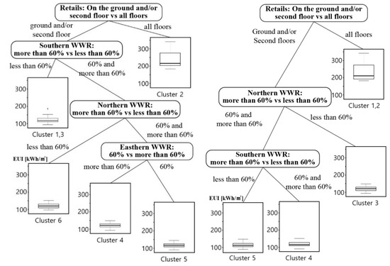
Figure 2.
Decision support models by k-means (left) and SOM (right).
5.3.3. GMM Clustering
To set an optimal number of GMM clusters, Bayesian information criteria (BIC) [67] were calculated by varying numbers of GMM clusters. Unfortunately, before PCA, only one cluster turned out be the best fit with the largest BIC. After PCA, nine clusters outputted a relatively high and stable BIC. Thus, the training set were divided into nine clusters. Compared to k-means or SOM clustering, each GMM cluster includes more longitudinally ranging EUIs (Figure 3), which signifies clearer splitting conditions could be obtained. Consequently, GMM clustering results in a lower variance of the clustered data at the leaf nodes as Figure 4 depicts, compared to k-mean or SOM clustering.

Figure 3.
GMM clustering before (left) and after (right) PCA.
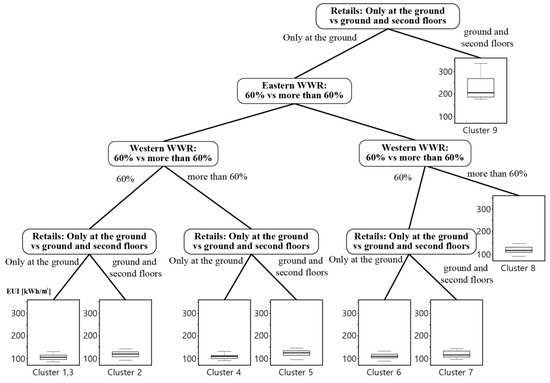
Figure 4.
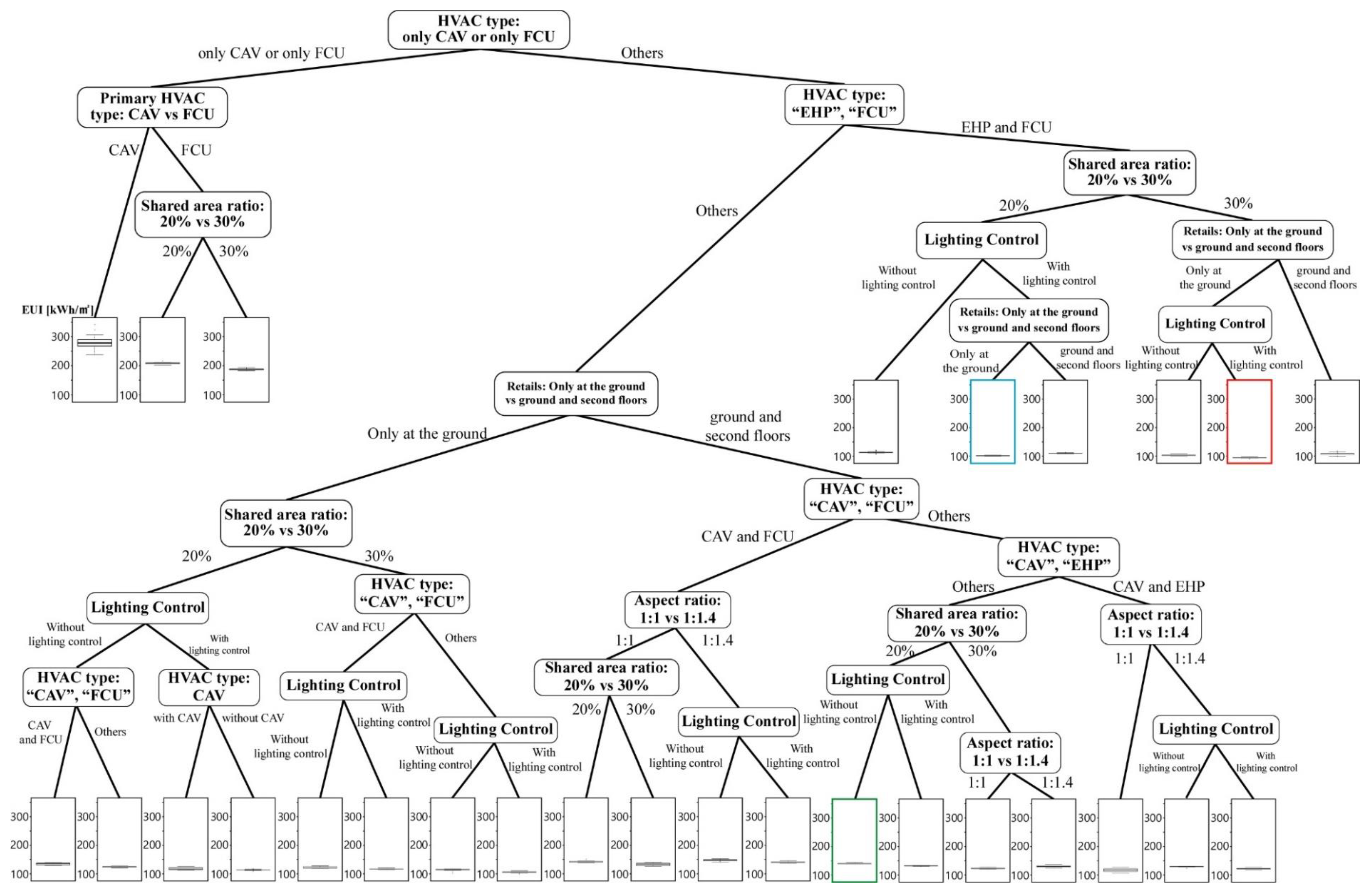
Decision support model by GMM.
5.4. Decision Support Models Developed by Decision Tree Algorithms
5.4.1. Single Tree Algorithms: CART and CIT
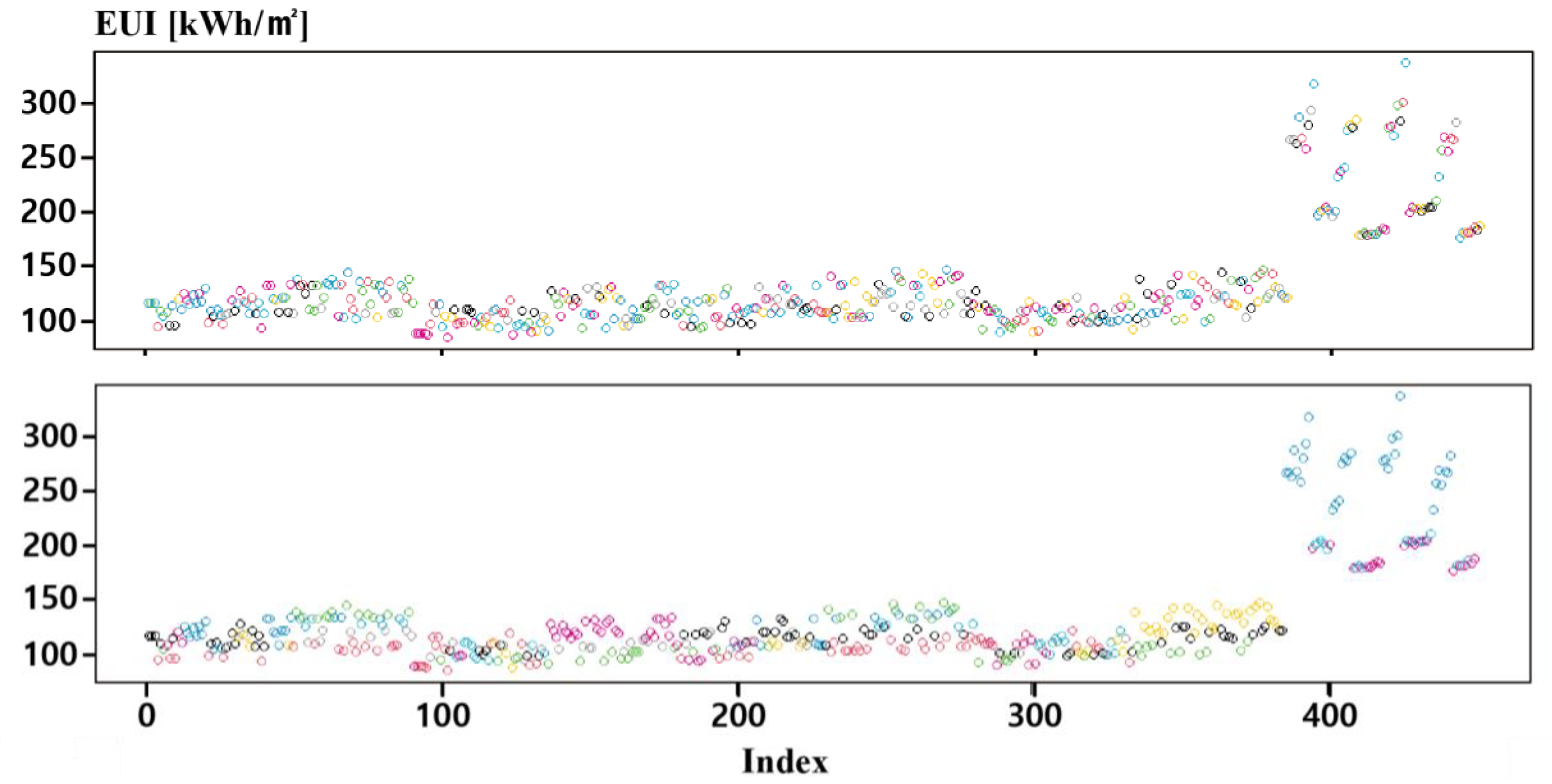
Figure 5 illustrates distributions of the training dataset by CART and CIT; each color indicates each cluster. Compared to clusters by CIT, the number of clusters by CART is smaller and each cluster has more lumped data. It is because the CIT decision tree (Figure 6) provides more splitting conditions compared to the CART decision tree (Figure 7). A more diverse combination of design variables for a similar EUI range was obtained using the CIT algorithm. Accordingly, the CIT algorithm produced a decision tree with less variance at the leaf nodes.
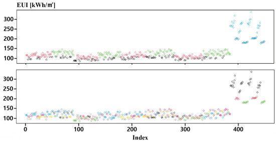
Figure 5.
CART clusters (top) and CIT clusters (bottom).
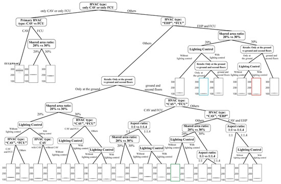
Figure 6.
Decision support model by CIT.

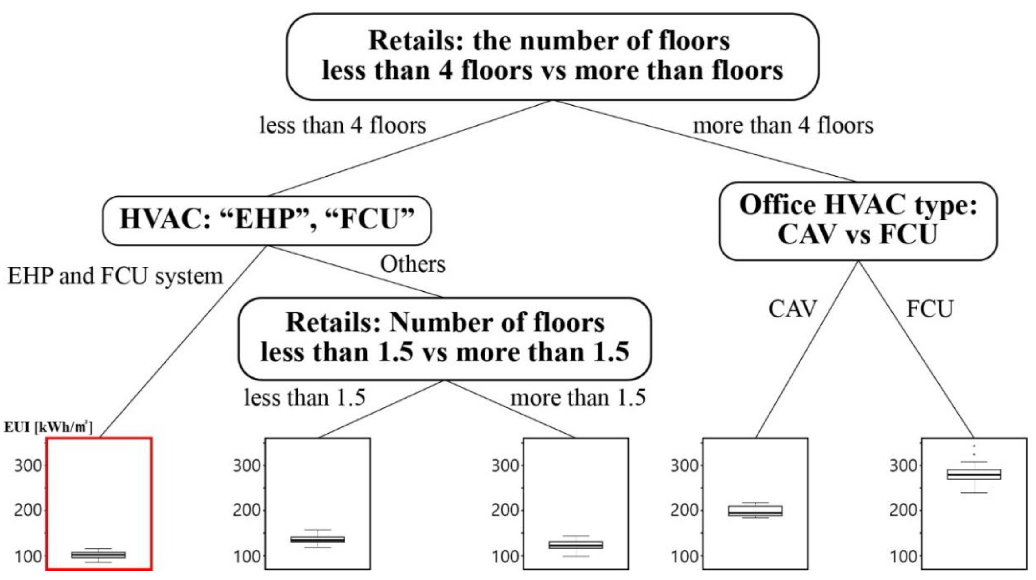
Figure 7.
Decision support model by CART.
The CART algorithm outputted a single decision tree in which facility zoning and the HVAC system were the only critical design variables; its smallest EUIs (80–120 kWh/m2) are found when the stores were on the ground or second floor, and the EHP and FCU service for stores and offices (the red line in Figure 7). In contrast, the CIT algorithm resulted in a single decision tree that first splits the HVAC system at the root node, and then splits the facility zoning, shared area ratio, lighting control, and aspect ratio, largely in order. Thus, its smallest EUIs (80 kWh/m2) were found at a more detailed condition—when the stores are only on the ground floor, the EHP and FCU service for stores and offices, respectively (HVAC #4), and the shared area ratio of the office floors is set to 30%, and lighting controls are enabled (the red line in Figure 6).
In addition, the CIT-based decision model intuitively displayed how much higher the EUI could be if the client chose other options instead of the smallest EUI options. For example, if the client wanted to place stores on both the ground and second floors and expand the rentable area (i.e., the shared area ratio decreased to 20%), the resulting EUI would be around 110 kWh/m2 as long as HVAC #4 and lighting control were selected (the blue line in Figure 6). However, without lighting control, the EUI would be as high as 120 kWh/m2. Additionally, if only FCUs were allowed, the EUI could reach 130 kWh/m2 with lighting control, and 140 kWh/m2 without it (the green line in Figure 6).
The CIT algorithm produced branching up to the 6th level, compared to only the 3rd level for the CART algorithm. This was because the CIT algorithm handles classification based on linear regression analysis, with most of the variables included in the linear regression model. Thus, even if the statistical significance is lower, classification continues, and the branch level increases. In contrast, because the CART algorithm performs classification by seeking to decrease the variance in the variables, classification stops if the variance is not reduced by a certain extent, leading to restricted branch levels.
When classifying the entire dataset, the CIT algorithm classifies the data by sorting a single variable based on the comprehensive judgment of all variables used for the linear regression analysis, whereas the CART algorithm classifies the data based on a single variable only. That is, even if it is falsely classified, the CIT algorithm continues classification when it is appropriate in terms of statistical significance, whereas the CART algorithm only performs classification based on sorting criteria that minimize the rate of false classification, meaning that branching is forcibly stopped if the classification criteria are not satisfied. Although the possibility of false classification is less likely to occur when using the CART algorithm, it ends with fewer design variables included in the final tree.
5.4.2. Forest Algorithms: RF and CIF
Compared to the clusters by CART and CIT, their forest algorithms resulted in more clusters and thus less data sets for each cluster (Figure 8). One remarkable observation is that the datasets by CIF algorithms tend to be longitudinally distributed within a cluster, whereas the datasets by RF algorithms are more scattered up and down within a cluster. This is because with the RF groups, the dataset is based on physical distance, whereas in the CIF group, the datasets are based on the significant test of a variable and its condition.
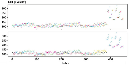
Figure 8.
RF clusters (top) and CIF clusters (bottom).
As decision forest algorithms employ random samplings to build single trees, the number of sample set (i.e., ntree) and the number of sampling features (i.e., mtry) should be set first. The number of sampling features was set to five because typically the square root of the number of all variables is recommended [68]. Additionally, ntree was set to two hundred because the OOB error starts to converge from two hundred rounds when it was varied.
In contrast to CART and CIT, RF and CIF are not visible as in a single tree, because decision forest algorithms calculate the (weighted) average of all the responses of member (single) trees for the given observation and then return it as the final prediction. Instead the important variable rank of all four tree algorithms are compared in Table 7. From the first to the fourth rank, RF, CIF and CIT resulted in the same variable importance. Furthermore, the four variables show a similar degree of importance. However, CART presented a different variable rank.

Table 7.
Top seven important variables by algorithm.
It implies that although RF and CIF may not have the same tree structure, the split conditions closer to the root node (which are the most critical) would be the same for both forests. In addition, it is more significant that the important variable rank of CIT does not differ from those of RF and CIF, which can be regarded as stable as forest algorithms.
5.5. Comparison of Prediction Accuracy
To verify the prediction accuracy of design decision models, fifty validation test cases that were likely to be observed in practice for the same test project were newly made. It means unrealistic design scenarios were not included for the test and there is no overlapped set of design variables.
For each decision support model, the difference between the mean EUI at the leaf node of the model and the EUIs obtained by simulating the test case using EnergyPlus were calculated, and then they were defined as error (%). The RMSE (Root Mean Square Error) and standard deviation of the errors were calculated using Equations (1) and (2), respectively.
where denotes the EUI of a test case using EnergyPlus; denotes the mean EUI of that test case estimated by a decision model; N denotes the number of test cases.
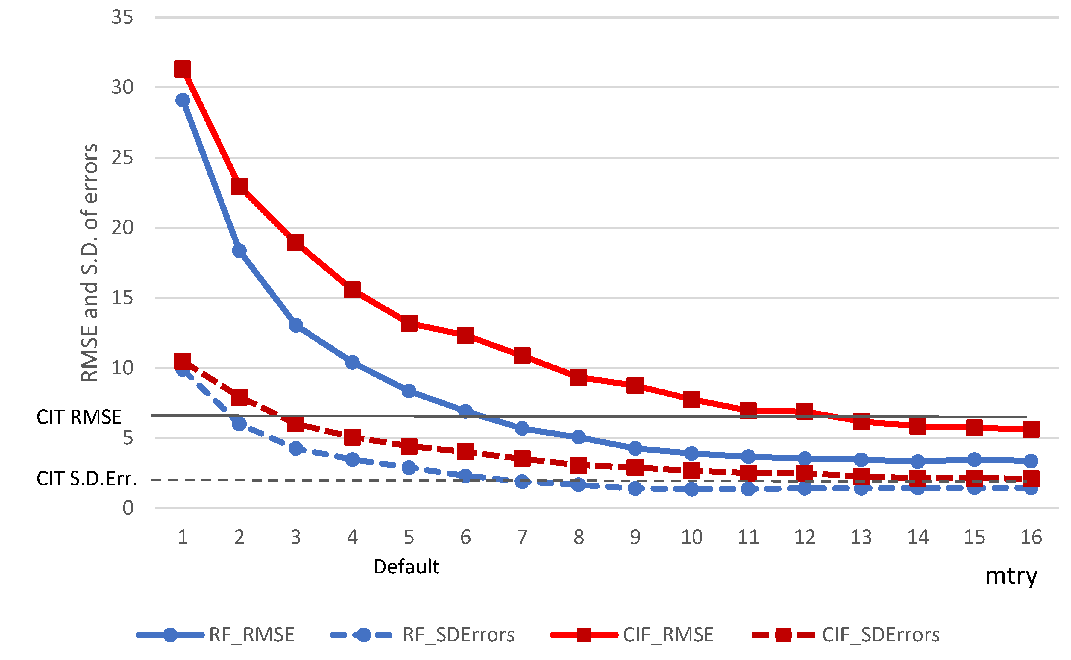
As shown in Table 8, CIT turned out to be the most accurate and precise among all the algorithms by having the lowest RMSE and standard deviation of errors. However, this result may go against a belief that in general, an RF algorithm has higher prediction accuracy than single tree algorithms [10]. Therefore, the number of sampling features (i.e., mtry) for RF were varied from one to sixteen. In addition, the same experiments were done for CIF. As Figure 9 depicted, when mtry increased to seven for RF (about 40% of feature variables) and fourteen for CIF (about 80% of feature variables), respectively, their RMSEs and standard deviations of errors began to drop under the RMSE and standard deviation of the errors by the CIT algorithm. The RMSE of RF drops to 4.0 as its mtry increases up to eleven (about 69% of feature variables), and then became stable after that. However, technically, the RMSE 4.0 would not make a dramatic accuracy difference from the RMSE 5.82. Increasing the mtry up to 69% of the feature variables is rather not recommended for forest algorithms due to increased computations.

Table 8.
RMSE and standard deviation of errors by algorithm.
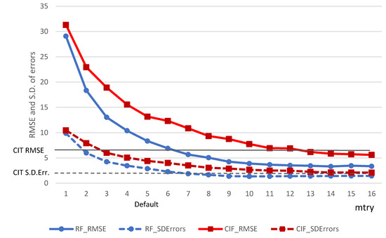
Figure 9.
RMSE and standard deviation of errors by RF and CIF algorithms upon the number of bagging features (mtry).
6. Discussion
6.1. Unsupervised vs. Supervised Algorithms
Clustering algorithms intentionally exclude heterogeneous data that deviate from the training dataset as outliers, assigning the data a meaningless likelihood (or distance) if the data deviate from the training dataset. Therefore, if test cases are observed in outlier zones, the prediction accuracy of clustering algorithms is likely to be lower. Because unsupervised algorithms, such as clustering, do not employ forced adjustment for subtle areas, their higher degree of freedom eventually leads to neutral data points being incorporated into the existing rules. Hence, unsupervised algorithms rather focus on identifying very distinct patterns or trends.
In contrast, decision-tree algorithms—a type of supervised algorithm—evaluate heterogeneous data against an object variable. For a set of outliers, as long as they meet the classification criteria (i.e., variance or test statistics) for a new condition, they form a new branch instead of being incorporated into existing classes. Consequently, this makes decision-tree algorithms more predictable than clustering algorithms. The principles of the tested tree and forest algorithms are discussed next.
6.1.1. Single Tree Algorithms: CART vs. CIT
When the training data used in this study were closely examined, the EUI was not always distributed continuously, and several regions were empty data spaces. As explained in Section 4.2.1, because the CART algorithm must create a branch that divides these no-data cavities, the split conditions for a no-data cavity cannot be sufficiently strict, which ultimately reduces the prediction accuracy. However, because the CIT algorithm represents a statistical approach to recursive partitioning, the prediction accuracy of CIT trees with early stopping is equivalent to the prediction accuracy of pruned trees with unbiased variable selection [58]. Therefore, the CIT algorithm can establish a marginal split condition that creates a border for no-data cavities without excessive branching.
6.1.2. Single Tree Algorithm and Its Forest Version: CART vs. RF
The prediction accuracy of the CART algorithm can be unstable depending on the training dataset because it is sensitive to noise in the training data. However, RF constructs trees through bootstrap aggregation, so it can compensate for this noise-driven instability by averaging the responses of multiple single trees. Therefore, RF should perform better than the CART algorithm in most cases in terms of prediction accuracy.
6.1.3. Single Tree Algorithm and Its Forest Version: CIT vs. CIF
The CIF is the forest version of the CIT algorithm, generalizing single-tree responses to reduce selection bias through bootstrap aggregation. However, because the CIF produces pruned single trees with only a small subset of features, its prediction accuracy can be lower than the CIT algorithm that selects a split measure based on the conditional distribution of the statistics using all the features. When the CIF selects bootstrapping features from no-data cavities and then produces member trees based on them, in particular, its prediction accuracy may fall.
6.1.4. Forest Algorithms: CIF vs. RF
As discussed in Section 4.2.3 and Section 4.2.4, CIF employs unbiased trees and sufficient resampling whereas RF favors variables with many potential cut points to rank the importance of the variables. However, the branch level for RF is typically a lot deeper than that for CIF because the CART algorithm (the member tree of RF) continues to develop lower branches until the reduction in the variance of the training data becomes zero (regardless of the variable type), whereas the CIT algorithm (the member tree of CIF) does so until no significant variable is observed. Therefore, when a sufficient number of features (mtry) is set for RF, the variance at its leaf nodes becomes smaller. Additionally, the average prediction at the leaf nodes of these member trees becomes more unbiased. This means that there is a trade-off between model complexity and prediction performance for RF.
6.1.5. CIT vs. RF in Terms of Accuracy and Interpretability
As mentioned above, when a sufficient number of features (mtry) and member trees (ntree) is employed for RF, it can outperform the CIT algorithm in terms of prediction accuracy. However, bootstrap aggregation improves prediction accuracy at the expense of interpretability. Although forest algorithms are statistically superior to single-tree algorithms, there is no single representative tree for all the training data, which means that forest algorithms may not be that different from black-box models in a perspective of decision maker. In addition to that, each member tree of RF (i.e., CART) tends to be over-fitted resulting in more than 25 levels of the leaf node hierarchy. It signifies that the model can be too complex to make decisions out of it.
Therefore, it is often recommended that the effect size of the split conditions be calculated using the ranking of variable importance from forest analysis, whereas the direction of the effect can be captured using a single-tree algorithm [69]. This recommendation is supported by the observation in the present study that the ranking of variable importance using the CIT algorithm did not differ greatly from that using RF and CIF (Table 7).
In summary, the CIT algorithm appears to be more appropriate than forest algorithms for EEB design decision support model at the feasibility analysis stage for the following reasons:
- I.
- Practical building designs are limited by the site conditions and context; thus, training data can be a mix of numerical, categorical, piecewise, and bipolar values. Additionally, features containing non-continuous data with many split points are not necessarily sensitive variables. In selecting split conditions, the CIT algorithm reduces the selection bias by separating the selection of the best covariate on which to make the split by searching for the best split point, even if there are covariates with many split points [70]. The CIT algorithm is thus applicable to all types of regression problems that incorporate a mix of nominal and numerical variables and multivariate response covariables [71], which is typical of architectural design cases. Consequently, the CIT algorithm is expected to exhibit a steady prediction performance for architectural design problems.
- II.
- During the feasibility analysis of a construction project, intuitively exploring design variables and their values is much more important than providing an accurate assessment of the expected performance of a specific alternative. That is, as many factors are indeterminant at this stage, the accuracy of a decision-support model rests on its ability to reasonably differentiate the expected performance of a particular option from that of an alternative, i.e., “classification accuracy”. The CIT algorithm has an acceptable classification accuracy, as the variance at its leaf nodes is within a reasonable range. Additionally, its interpretability is far superior to that of forest algorithms. Thus, decision-makers can quickly identify with reasonable confidence what groups of design variables should be selected initially to meet the objectives and what values they should take.
6.2. Use Case of the CIT-Based Decision Support Model and Future Applications
If an expert constructs a database with a suitable collection of design variables and a reasonable range of options (i.e., the economic constraints and energy compliance regulations in Figure 1) in advance by considering factors such as the building type, size, and site characteristics, the proposed CIT-based decision-support model could be implemented as an inference engine for an expert system and/or a supplemental map for design optimization. The expert system can then be employed by an EEB consultant to make decisions during the very early design stages or can act as a substitute for the expert in some situations. Public users of the expert system—the architect and client—do not need to identify candidate variables and options themselves. Instead, they only need to compare the performance and economics of options from an exhaustive database of assorted design combinations prepared by experts and then choose their preferred choice. Additionally, using the proposed CIT-based decision-support model as a supplemental “map” for design optimization, users can take an advantage of the convenient and fast solutions provided by the optimizer, while also being told how the optimal solution was derived. This expert system is thus expected to be more suitable for buildings whose setup can be standardized to some degree. Examples of these buildings include educational institutions, apartment complexes, small and mid-sized commercial buildings, and dormitories.
7. Conclusions
In the EEB design process, EEB decision-makers usually employ building simulations for case-specific designs to quantitatively evaluate which design variables affect the performance and how the synergy or dysergy between the design variables affects performance. However, at the very early stage, there is generally a lack of sufficient detail to run accurate simulations, and specifications for the building and system may not yet be sufficiently well-defined. Thus, instead of using simulations to quantify the trade-off between the performance and cost of design alternatives, practitioners tend to make early-stage decisions with the support of consultants who have experience with similar projects. However, small and mid-sized projects may not be able to afford these consultants.
If a reasonable collection of design variables and options for project context are available in a database, a meta-model can be constructed using many simulation runs of various design combinations retrieved from the database. This meta-model can thus act as a decision-support model during the very early stages of the design process. Decision-makers who could not afford the cost, time, or manpower required for simulation analysis can benefit from this useful design support.
At the feasibility analysis stage, where design exploration is much more important than developing details of selected alternatives, a more transparent and interpretable design support model is more advantageous in design decision-making, with designers preferring transparent and interactive methods to black-box methods such as optimization. Furthermore, a decision-support model at the feasibility analysis stage requires an accuracy that allows the expected performance of a particular option to be reasonably differentiated from that of an alternative, i.e., classification accuracy.
Most meta-models utilized in previous studies, such as ANNs and GPMs, are opaque because these machine-learning models are generally known to be more accurate in terms of prediction. Therefore, this study aims to identify a machine-learning algorithm that could be used to develop a transparent meta-model with reasonable classification accuracy. Unsupervised clustering algorithms (hierarchical clustering, k-means, SOM, and GMM) and supervised decision-tree algorithms (CART, CIT, RF, and CIF) were tested using training cases collected from an actual new building project. The accuracy of the energy performance predicted by the eight decision models was validated and compared using real test cases. The comparison results showed that the CIT-based model had a reasonable classification accuracy and superior interpretability for the energy performance of the building.
Although training and verification datasets were obtained from a real construction context, its design options may not be realistic from a perspective of practitioner. Thereby, more realistic architectural scenarios and engineering design cases need to be tested to enhance the robustness of the proposed CIT-based decision support model.
Nevertheless, for a mix of numerical and nominal values, the CIT-based model is expected to demonstrate a consistent prediction performance. Furthermore, it can be used as the inference engine within an expert system that can be employed by an EEB consultant at very early design stages or can even replace the role of an expert if required. It can also act as a supplementary map for an optimizer by explaining how the optimal solution was obtained. It is believed that an expert system with a CIT-based decision-support model is best suited for buildings whose setup can be standardized to some degree, including educational institutions, apartment complexes, small and mid-sized commercial buildings, and dormitories.
Author Contributions
Conceptualization, S.H.K.; methodology, S.H.K.; investigation, S.Y.C. and S.H.K.; data curation, S.Y.C.; writing, S.Y.C. and S.H.K.; project administration, S.H.K.; funding acquisition, S.H.K. All authors have read and agreed to the published version of the manuscript.
Funding
This work was supported by the National Research Foundation of Korea (NRF) grant funded by the Korea government (MSIT) (No. 2020R1A2C1012952).
Institutional Review Board Statement
Not applicable.
Informed Consent Statement
Not applicable.
Data Availability Statement
Not applicable.
Acknowledgments
Not applicable.
Conflicts of Interest
Not applicable.
References
- Schade, J.; Olofsson, T.; Schreyer, M. Decision-making in a model-based design process. Constr. Manag. Econ. 2011, 29, 371–382. [Google Scholar] [CrossRef]
- Østergård, T.; Jensen, R.L.; Maagaard, S.E. Building simulations supporting decision making in early design—A review. Renew. Sustain. Energy Rev. 2016, 61, 187–201. [Google Scholar] [CrossRef]
- Bektas, E.B.; Aksoy, U.T. Prediction of building energy needs in early stage of design by using ANFIS. Expert Syst. Appl. 2011, 38, 5352–5358. [Google Scholar] [CrossRef]
- Braganca, L.; Vieira, S.M.; Andrade, J.B. Early Stage Design Decisions: The Way to Achieve Sustainable Buildings at Lower Costs. Sci. World J. 2014, 2014, 365364. [Google Scholar] [CrossRef] [PubMed]
- Alsaadani, S.; Bleil, D.S.C. Performer, consumer or expert? A critical review of building performance simulation training paradigms for building design decision-making. J. Build. Perform. Simul. 2019, 12, 289–307. [Google Scholar] [CrossRef]
- Tian, W. A review of sensitivity analysis methods in building energy analysis. Renew. Sustain. Energy Rev. 2013, 20, 411–419. [Google Scholar] [CrossRef]
- Machairas, V.; Tsangrassoulis, A.; Axarli, K. Algorithms for optimization of building design: A review. Renew. Sustain. Energy Rev. 2014, 31, 101–112. [Google Scholar] [CrossRef]
- Tian, Z.; Zhang, X.; Jin, X.; Zhou, X.; Si, B.; Shi, X. Towards adoption of building energy simulation and optimization for pas-sive building design: A survey and a review. Energy Build. 2018, 158, 1306–1316. [Google Scholar] [CrossRef]
- Eisenhower, B.; O’Neill, Z.; Narayanan, S.; Fonoberov, V.A.; Mezić, I. A methodology for meta-model based optimization in building energy models. Energy Build. 2012, 47, 292–301. [Google Scholar] [CrossRef]
- Østergård, T.; Jensen, R.L.; Maagaard, S.E. A comparison of six metamodeling techniques applied to building performance simulations. Appl. Energy 2018, 211, 89–103. [Google Scholar] [CrossRef]
- Chen, X.; Yang, H.; Sun, K. Developing a meta-model for sensitivity analyses and prediction of building performance for pas-sively designed high-rise residential buildings. Appl. Energy 2017, 194, 422–439. [Google Scholar] [CrossRef]
- Westermann, P.; Evins, R. Surrogate modelling for sustainable building design—A review. Energy Build. 2019, 198, 170–186. [Google Scholar] [CrossRef]
- Østergård, T.; Jensen, R.L.; Maagaard, S.E. Early Building Design: Informed decision-making by exploring multidimensional design space using sensitivity analysis. Energy Build. 2017, 142, 8–22. [Google Scholar] [CrossRef]
- Tian, W.; Choudhary, R.; Augenbroe, G.; Lee, S.H. Importance analysis and meta-model construction with correlated variables in evaluation of thermal performance of campus buildings. Build. Environ. 2015, 92, 61–74. [Google Scholar] [CrossRef]
- Edwards, R.; New, J.; Parker, L.; Cui, B.; Dong, J. Constructing Large Scale Surrogate Models from Big Data and Artificial Intelligence. Appl. Energy 2017, 202, 685–699. [Google Scholar] [CrossRef]
- Romani, Z.; Draoui, A.; Allard, F. Metamodeling the heating and cooling energy needs and simultaneous building envelope optimization for low energy building design in Morocco. Energy Build. 2015, 102, 139–148. [Google Scholar] [CrossRef]
- Ascione, F.; Bianco, N.; De, S.C.; Mauro, M.G.; Vanoli, G.P. Artificial neural networks to predict energy performance and ret-rofit scenarios for any member of a building category: A novel approach. Energy 2017, 118, 999–1017. [Google Scholar] [CrossRef]
- Singaravel, S.; Suykens, J.; Geyer, P. Deep-learning neural-network architectures and methods: Using component-based mod-els in building-design energy prediction. Adv. Eng. Inform. 2018, 38, 81–90. [Google Scholar] [CrossRef]
- Asadi, E.; Silva, M.G.D.; Antunes, C.H.; Dias, L.; Glicksman, L. Multi-objective optimization for building retrofit: A model using genetic algorithm and artificial neural network and an application. Energy Build. 2014, 81, 444–456. [Google Scholar] [CrossRef]
- Rackes, A.; Melo, A.P.; Lamberts, R. Naturally comfortable and sustainable: Informed design guidance and performance la-beling for passive commercial buildings in hot climates. Appl. Energy 2016, 174, 256–274. [Google Scholar] [CrossRef]
- Tsanas, A.; Xifara, A. Accurate quantitative estimation of energy performance of residential buildings using statistical machine learning tools. Energy Build. 2012, 49, 560–567. [Google Scholar] [CrossRef]
- Chen, X.; Yang, H. Integrated energy performance optimization of a passively designed high-rise residential building in dif-ferent climatic zones of China. Appl. Energy 2018, 215, 145–158. [Google Scholar] [CrossRef]
- Kim, Y.J. Comparative study of surrogate models for uncertainty quantification of building energy model: Gaussian Process Emulator vs. Polynomial Chaos Expansion. Energy Build. 2016, 133, 46–58. [Google Scholar] [CrossRef]
- Rivalin, L.; Stabat, P.; Marchio, D.; Caciolo, M.; Hopquin, F. A comparison of methods for uncertainty and sensitivity analysis applied to the energy performance of new commercial buildings. Energy Build. 2018, 166, 489–504. [Google Scholar] [CrossRef]
- Prada, A.; Gasparella, A.; Baggio, P. On the performance of meta-models in building design optimization. Appl. Energy 2018, 225, 814–826. [Google Scholar] [CrossRef]
- Yang, S.; Tian, W.; Cubi, E.; Meng, Q.; Liu, Y.; Wei, L. Comparison of Sensitivity Analysis Methods in Building Energy Assessment. Procedia Eng. 2016, 146, 174–181. [Google Scholar] [CrossRef]
- Wortmann, T. Genetic Evolution vs. Function Approximation: Benchmarking Algorithms for Architectural Design Optimiza-tion. J. Comput. Des. Eng. 2018, 6, 414–428. [Google Scholar] [CrossRef]
- Van, G.L.; Das, P.; Janssen, H.; Roels, S. Comparative study of metamodelling techniques in building energy simulation: Guidelines for practitioners. Simul. Model. Pract. Theory 2014, 49, 245–257. [Google Scholar]
- Wei, Y.; Zhang, X.; Shi, Y.; Xia, L.; Pan, S.; Wu, J.; Han, M.; Zhao, X. A review of data-driven approaches for prediction and classification of building energy consumption. Renew. Sustain. Energy Rev. 2018, 82, 1027–1047. [Google Scholar] [CrossRef]
- Brown, N.C. Design performance and designer preference in an interactive, data-driven conceptual building design scenario. Des. Stud. 2020, 68, 1–33. [Google Scholar] [CrossRef]
- Bryant, F.B.; Yarnold, P.R. Principal-Components Analysis and Exploratory and Confirmatory Factor Analysis; American Psychological Association: Washington, DC, USA, 1995. [Google Scholar]
- Unsupervised Learning. 2022. Available online: https://en.wikipedia.org/wiki/Unsupervised_learning (accessed on 19 February 2022).
- Markowska-Kaczmar, U.; Kwasnicka, H.; Paradowski, M. Intelligent Techniques in Personalization of Learning in e-Learning Sys-tems; Springer: Berlin, Heidelberg, 2010. [Google Scholar] [CrossRef]
- Johnston, B.; Jones, A.; Kruger, C. Applied Unsupervised Learning with Python: Discover Hidden Patterns and Relationships in Unstructured Data with Python; Packt: Birmingham, UK, 2019; ISBN 978-1-78995-229-2. [Google Scholar]
- Abbas, O.A. Comparisons Between Data Clustering Algorithms. Int. Arab J. Inf. Technol. 2008, 5, 320–325. [Google Scholar]
- Günter, S.; Bunke, H. Self-organizing map for clustering in the graph domain. Pattern Recognit. Lett. 2002, 23, 405–417. [Google Scholar] [CrossRef]
- Mengjie, H.; Zhenwu, W.; Xingxing, Z. An Approach to Data Acquisition for Urban Building Energy Modeling Using a Gauss-ian Mixture Model and Expectation-Maximization Algorithm. Buildings 2021, 11, 30. [Google Scholar] [CrossRef]
- Bourdeau, M.; Zhai, X.Q.; Nefzaoui, E.; Guo, X.; Chatellier, P. Modeling and forecasting building energy consumption: A review of data-driven techniques. Sustain. Cities Soc. 2019, 48, 101533. [Google Scholar] [CrossRef]
- Yu, Z.; Haghighat, F.; Fung, B.C.M.; Yoshino, H. A decision tree method for building energy demand modeling. Energy Build. 2010, 42, 1637–1646. [Google Scholar] [CrossRef]
- Li, Z.Y. An Empirical Study of Knowledge Discovery on Daily Electrical Peak Load Using Decision Tree. Adv. Mater. Res. 2012, 433–440, 4898–4902. [Google Scholar] [CrossRef]
- Mikučionienė, R.; Martinaitis, V.; Keras, E. Evaluation of energy efficiency measures sustainability by decision tree method. Energy Build. 2014, 76, 64–71. [Google Scholar] [CrossRef]
- Pang, Y.; Jiang, X.; Zou, F.; Gan, Z.; Wang, J. Research on Energy Consumption of Building Electricity Based on Decision Tree Algorithm. In Euro-China Conference on Intelligent Data Analysis and Applications; Springer: Cham, Switzerland, 2018. [Google Scholar]
- Ahmad, M.W.; Mourshed, M.; Rezegui, Y. Trees vs. Neurons: Comparison between random forest and ANN for high-resolution prediction of building energy consumption. Energy Build. 2017, 147, 77–89. [Google Scholar] [CrossRef]
- Tso, G.K.F.; Yau, K.K.W. Predicting electricity energy consumption: A comparison of regression analysis, decision tree and neural networks. Energy 2007, 32, 1761–1768. [Google Scholar] [CrossRef]
- Wang, Z.; Wang, Y.; Zeng, R.; Srinivasan, R.S.; Ahrentzen, S. Random Forest based hourly building energy prediction. Energy Build. 2018, 171, 11–25. [Google Scholar] [CrossRef]
- Marijana, Z.S.; Adela, H.; Marinela, K. Predicting energy cost of public buildings by artificial neural networks, CART and random forest. Neurocomputing 2021, 439, 223–233. [Google Scholar]
- Cheng, F.W.; Gao, X.; Bao, L.; Mitchell, D.C.; Wood, C.; Sliwinski, M.J.; Smiciklas-Wright, H.; Still, C.D.; Rolston, D.D.K.; Jensen, G.L. Obesity as a risk factor for developing functional limitation among older adults: A conditional inference tree analysis. Obesity 2017, 25, 1263–1269. [Google Scholar] [CrossRef] [Green Version]
- Schivinski, B. Eliciting brand-related social media engagement: A conditional inference tree framework. J. Bus. Res. 2021, 130, 594–602. [Google Scholar] [CrossRef]
- Venkatasubramaniam, A.; Wolfson, J.; Mitchell, N.; Barnes, T.; JaKa, M.; French, S. Decision trees in epidemiological research. Emerg. Themes Epidemiol. 2017, 14, 11. [Google Scholar] [CrossRef]
- Sathishkumar, V.E.; Park, J.; Cho, Y. Using data mining techniques for bike sharing demand prediction in metropolitan city. Comput. Commun. 2020, 153, 353–366. [Google Scholar] [CrossRef]
- Wei, F.; Jeffrey, S. Simonoff, Unbiased regression trees for longitudinal and clustered data. Comput. Stat. Data Anal. 2015, 88, 53–74. [Google Scholar] [CrossRef]
- Breiman, L.; Friedman, J.H.; Olshen, R.A.; Stone, C.J. Classification and Regression Trees; Wadsworth & Brooks/Cole Advanced Books & Software: Monterey, CA, USA, 1984; ISBN 978-0-412-04841-8. [Google Scholar]
- Quinlan, J.R. C4.5: Programs for Machine Learning; Morgan Kaufmann Publishers: San Francisco, CA, USA, 1993. [Google Scholar]
- Hothorn, T.; Hornik, K.; Zeileis, A. Unbiased Recursive Partitioning: A Conditional Inference Framework. J. Comput. Graph. Stat. 2006, 15, 651–674. [Google Scholar] [CrossRef]
- Das, A.; Abdel-Aty, M.; Pande, A. Using conditional inference forests to identify the factors affecting crash severity on arterial corridors. J. Saf. Res. 2009, 40, 317–327. [Google Scholar] [CrossRef]
- Hastie, T.; Tibshirani, R.; Friedman, J. The Elements of Statistical Learning, 2nd ed.; Springer: Berlin, Germany, 2008; ISBN 0-387-95284-5. [Google Scholar]
- James, G.; Witten, D.; Hastie, T.; Tibshirani, R. An Introduction to Statistical Learning, 1st ed.; Springer: New York, NY, USA, 2013. [Google Scholar] [CrossRef]
- Strobl, C.; Boulesteix, A.L.; Kneib, T.; Augustin, T.; Zeileis, A. Conditional variable importance for random forests. BMC Bioin-form. 2008, 9, 307. [Google Scholar] [CrossRef]
- Strobl, C.; Boulesteix, A.L.; Zeileis, A.; Hothorn, T. Bias in random forest variable importance measures: Illustrations, sources and a solution. BMC Bioinform. 2007, 8, 25. [Google Scholar] [CrossRef]
- Xia, R. Comparison of Random Forests and Cforest: Variable Importance Measures and Prediction Accuracies. Master’s Thesis, Utah State University, Logan, UT, USA, 2009. Available online: https://digitalcommons.usu.edu/gradreports/1255/ (accessed on 19 February 2022).
- R Core Team. R: A Language and Environment for Statistical Computing; R Foundation for Statistical Computing: Vienna, Austria, 2022; Available online: https://www.R-project.org/ (accessed on 19 February 2022).
- Ministry of Land, Infrastructure and Transport (2022. 02), Enforcement Decree of the National Land Planning and Utilization Act. Available online: https://www.law.go.kr (accessed on 19 February 2022).
- Korea Agency for Technology and Standards, KS F 2292 Window Sets. Available online: https://e-ks.kr/streamdocs/view/sd;streamdocsId=72059237883883561 (accessed on 18 August 2022).
- Loh, W.L. On Latin hypercube sampling. Ann. Stat. 1996, 24, 2058–2080. [Google Scholar] [CrossRef]
- EnergyPlus. 2022. Available online: https://energyplus.net (accessed on 19 February 2022).
- Korea Energy Agency, Building Energy Efficiency Rating Certification System Operational Regulations. Available online: https://beec.energy.or.kr (accessed on 19 February 2022).
- Bayesian Information Criterion. 2022. Available online: https://en.wikipedia.org/wiki/Bayesian_information_criterion (accessed on 19 February 2022).
- Yang, X.S. 6—Data mining techniques. In Introduction to Algorithms for Data Mining and Machine Learning; Yang, X.-S., Ed.; Academic Press: Orlando, FL, USA, 2019; pp. 109–128. [Google Scholar]
- Tagliamonte, S.; Baayen, R. Models, forests, and trees of York English: Was/were variation as a case study for statistical practice. Lang. Var. Change 2012, 24, 135–178. [Google Scholar] [CrossRef]
- Johnstone, C.P.; Lill, A.; Reina, R.D. Habitat loss, fragmentation and degradation effects on small mammals: Analysis with conditional inference tree statistical modelling. Biol. Conserv. 2014, 176, 80–98. [Google Scholar] [CrossRef]
- Hothorn, T.; Hornik, K.; Zeileis, A. Ctree: Conditional Inference Trees. The Comprehensive R Archive Network. 2020. Available online: https://cran.r-project.org/web/packages/partykit/vignettes/ctree.pdf (accessed on 19 February 2022).
Publisher’s Note: MDPI stays neutral with regard to jurisdictional claims in published maps and institutional affiliations. |
© 2022 by the authors. Licensee MDPI, Basel, Switzerland. This article is an open access article distributed under the terms and conditions of the Creative Commons Attribution (CC BY) license (https://creativecommons.org/licenses/by/4.0/).

