
Numerical Prediction of Turbulent Drag Reduction with Different Solid Fractions and Distribution Shapes over Superhydrophobic Surfaces


Abstract
:1. Introduction
2. Computational Approach and Numerical Methods
3. Results and Discussion
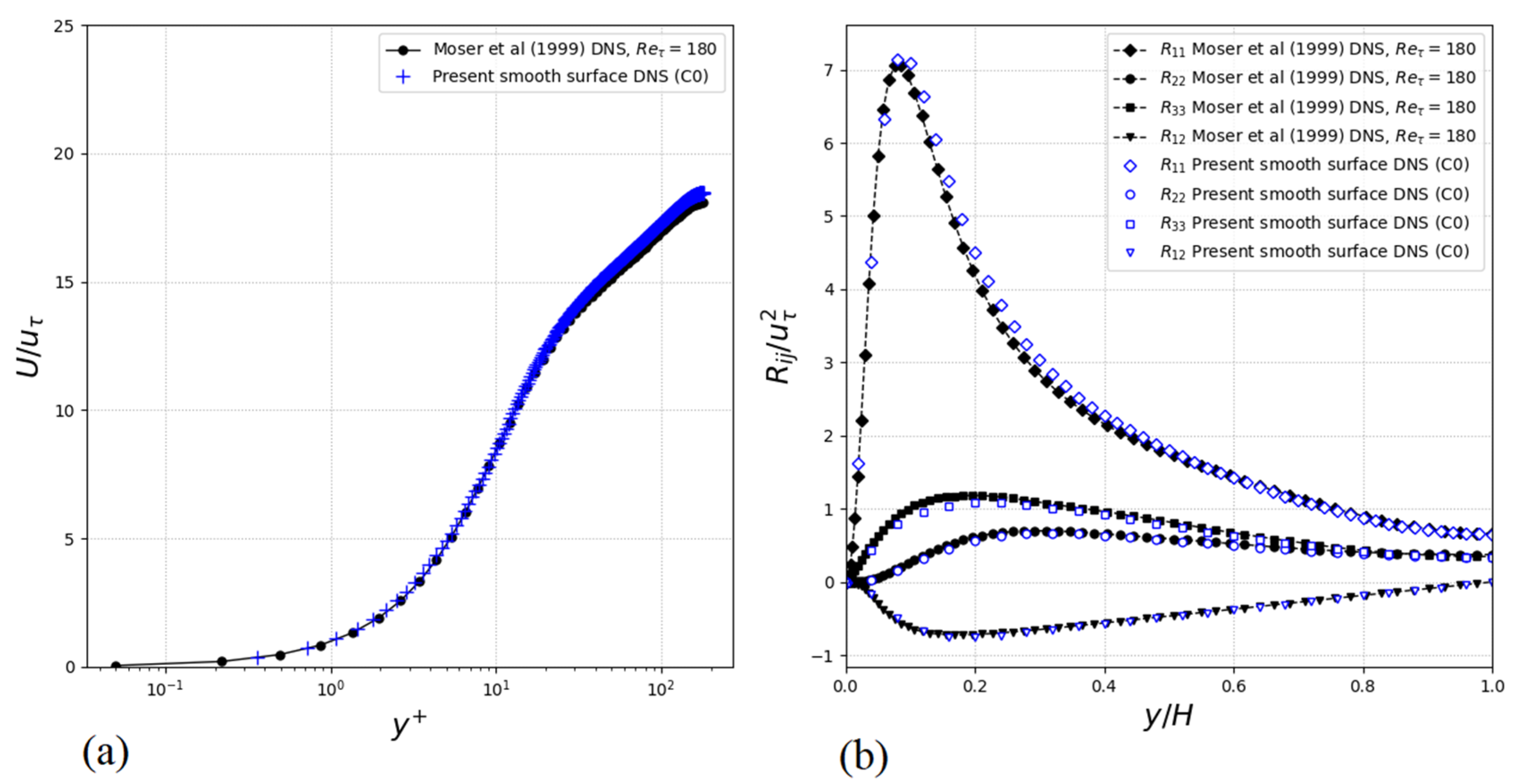
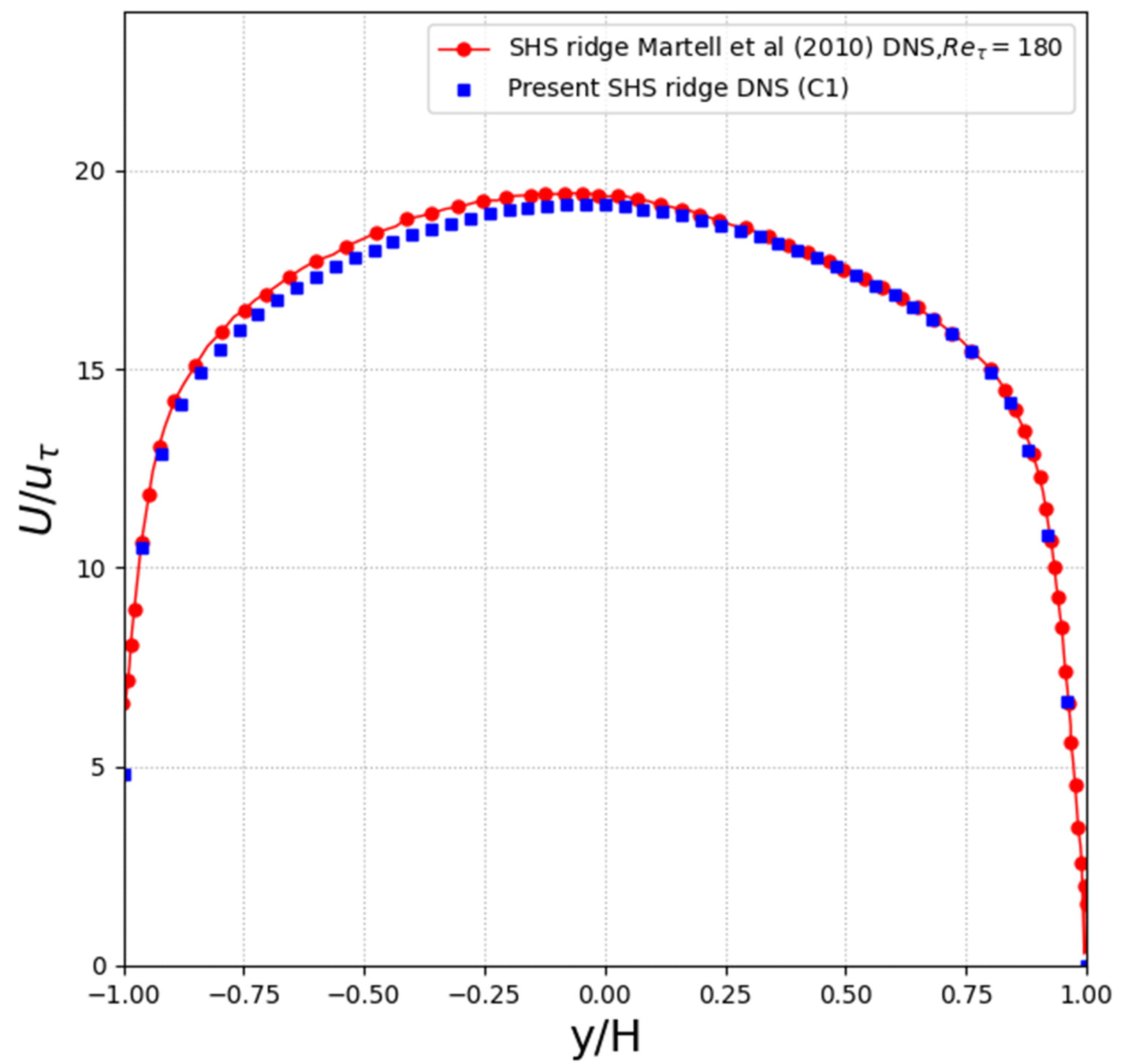
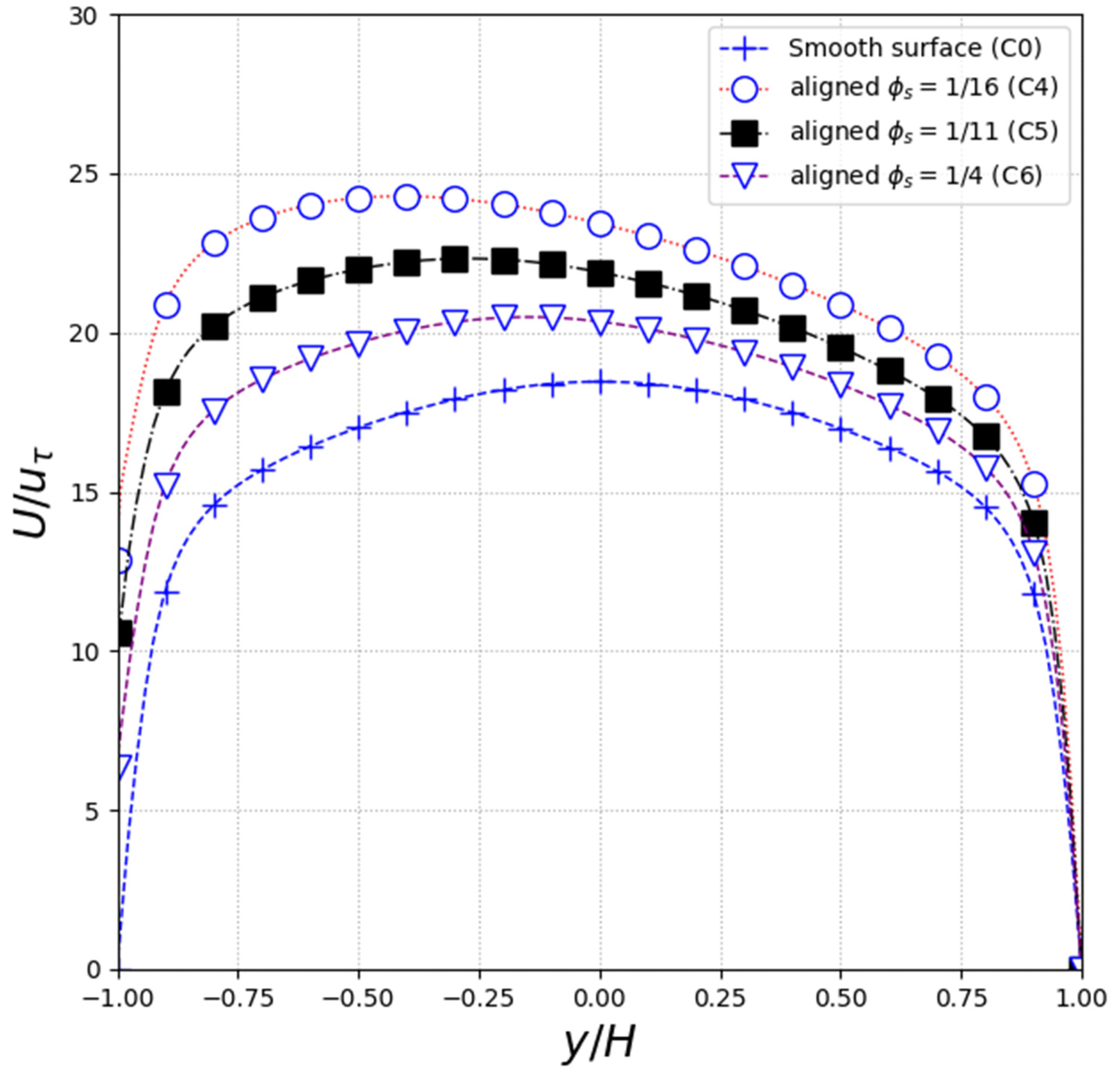
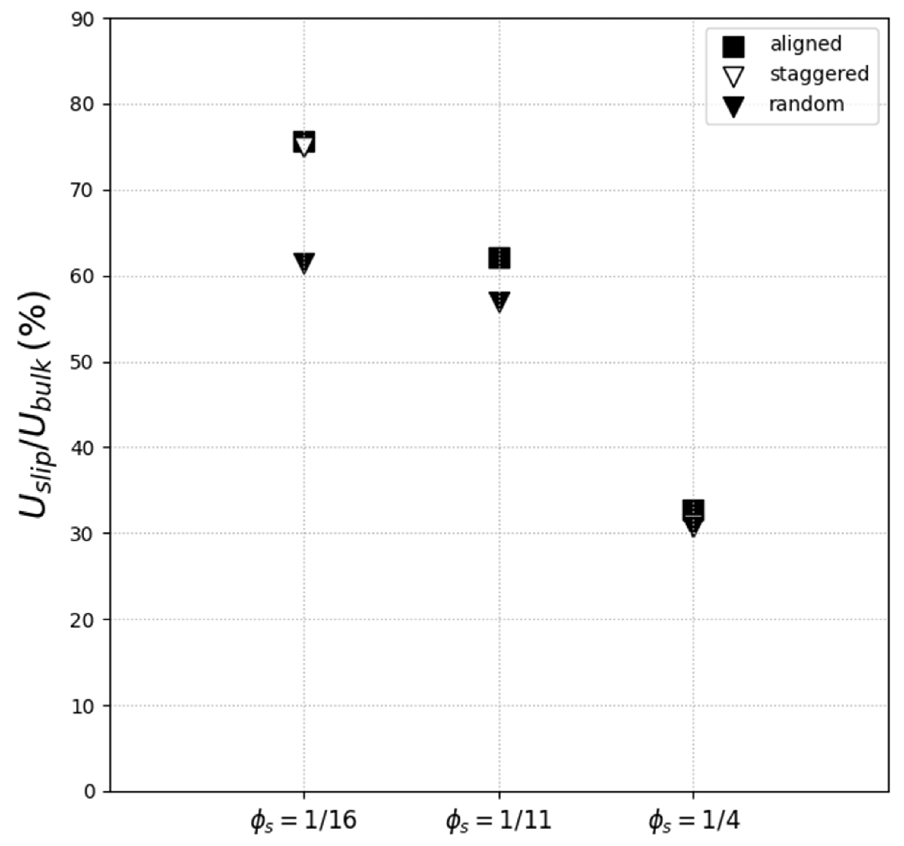
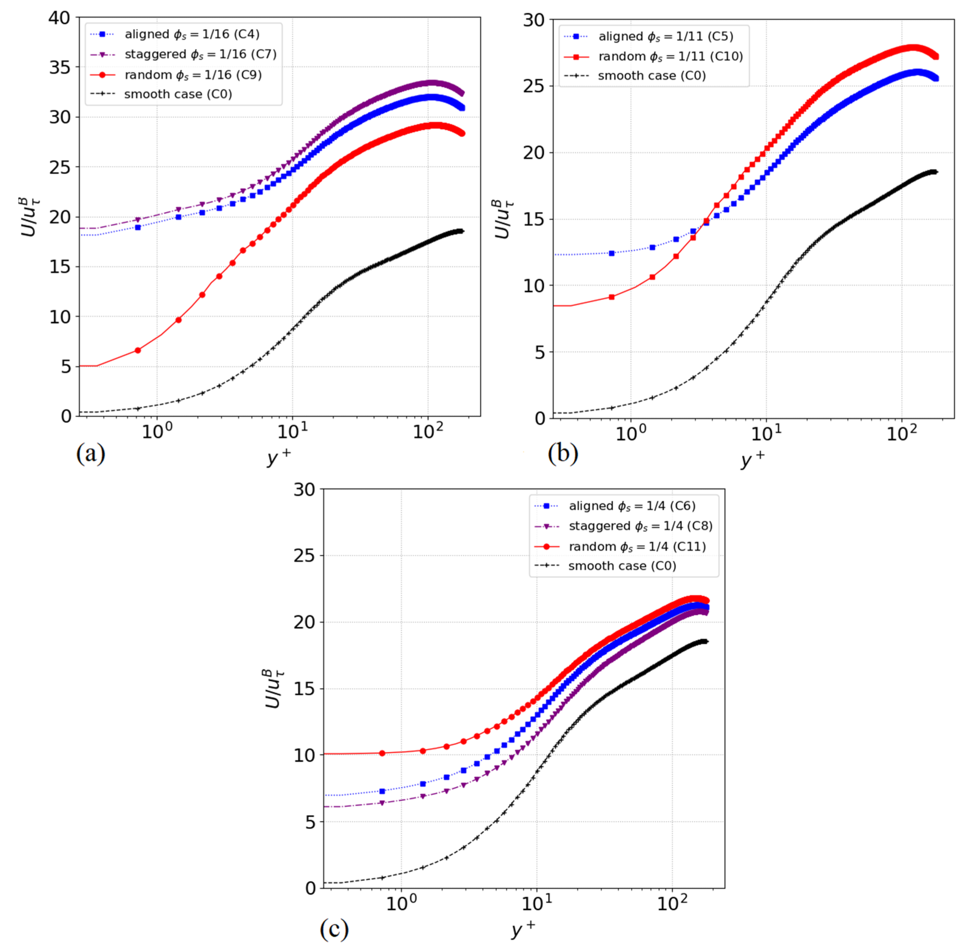
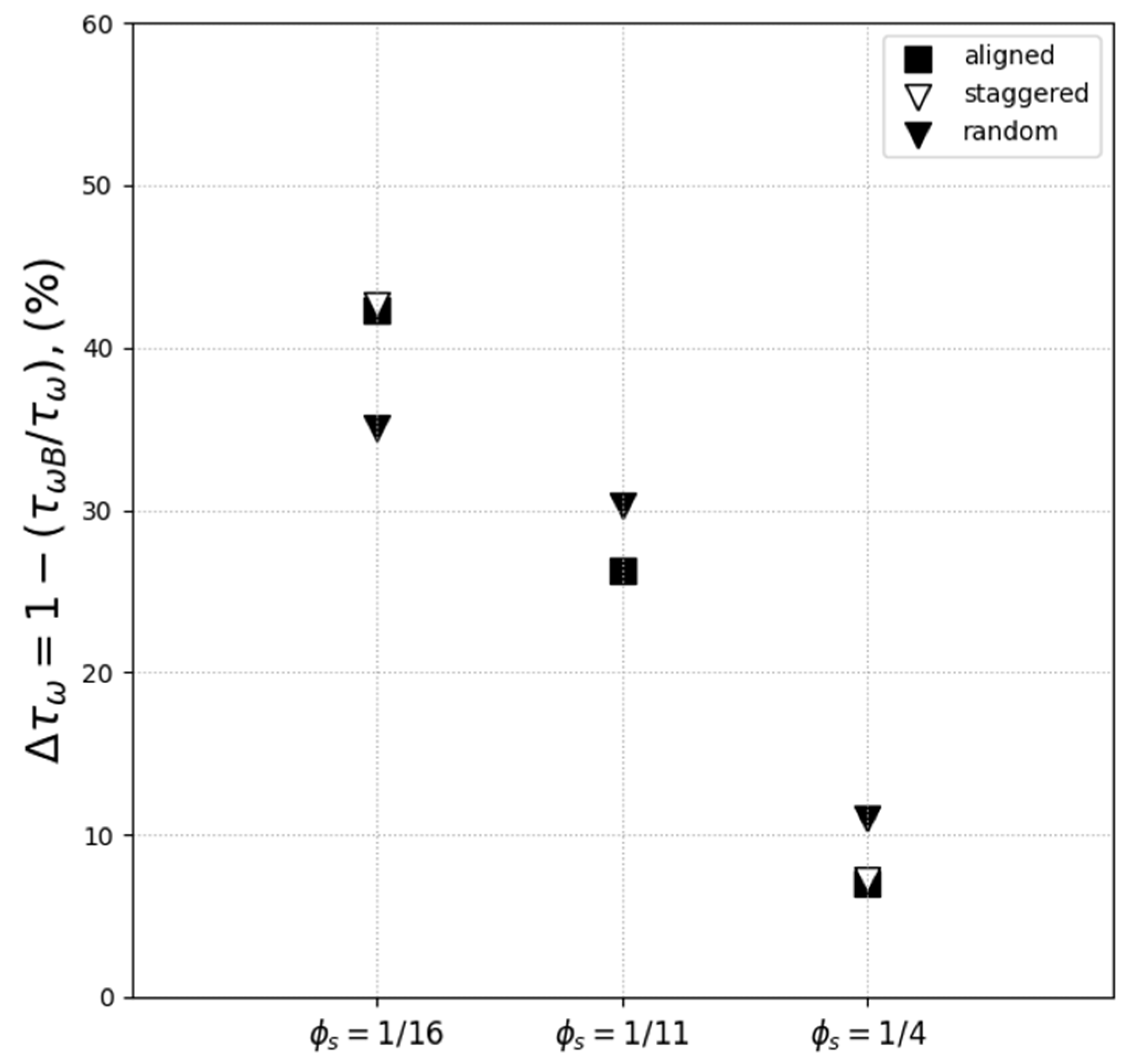
3.1. Drag Reduction and Mean Velocity Profile
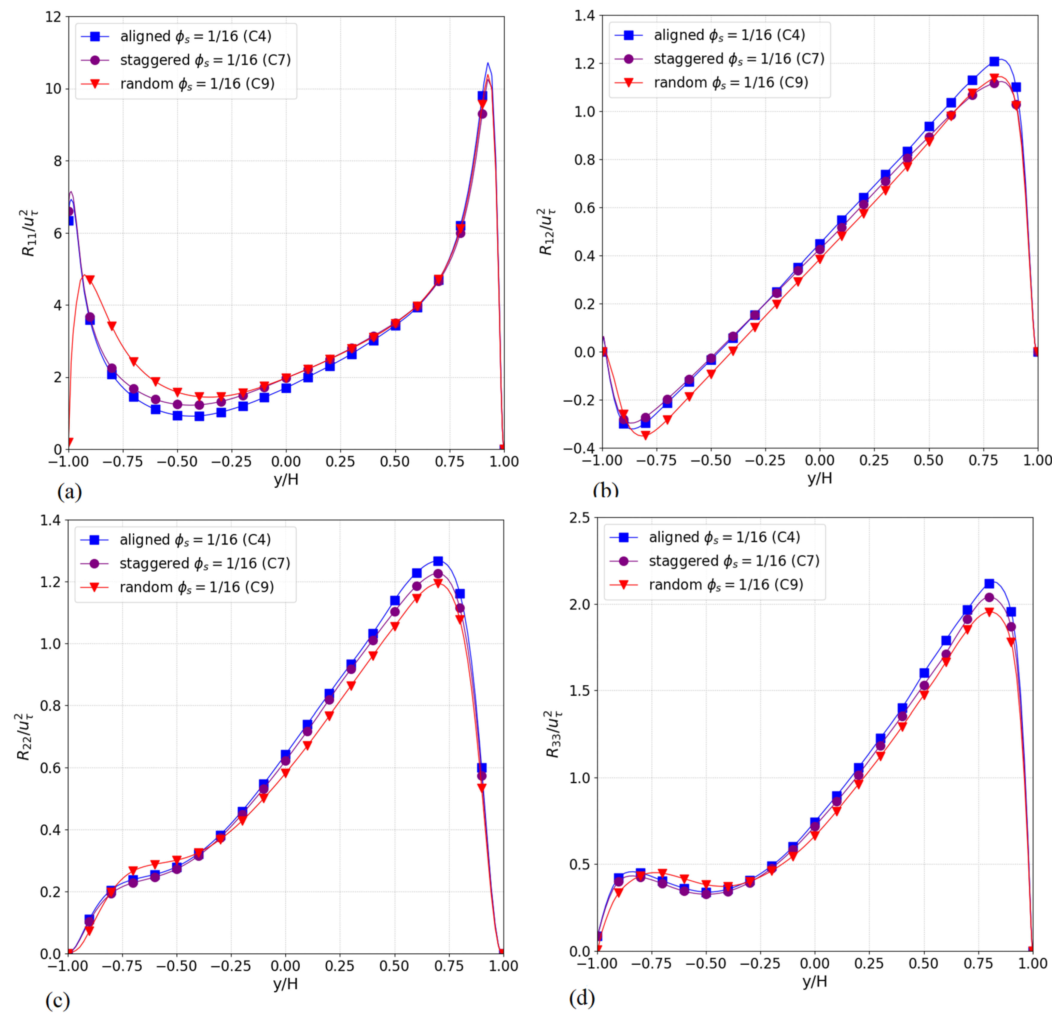
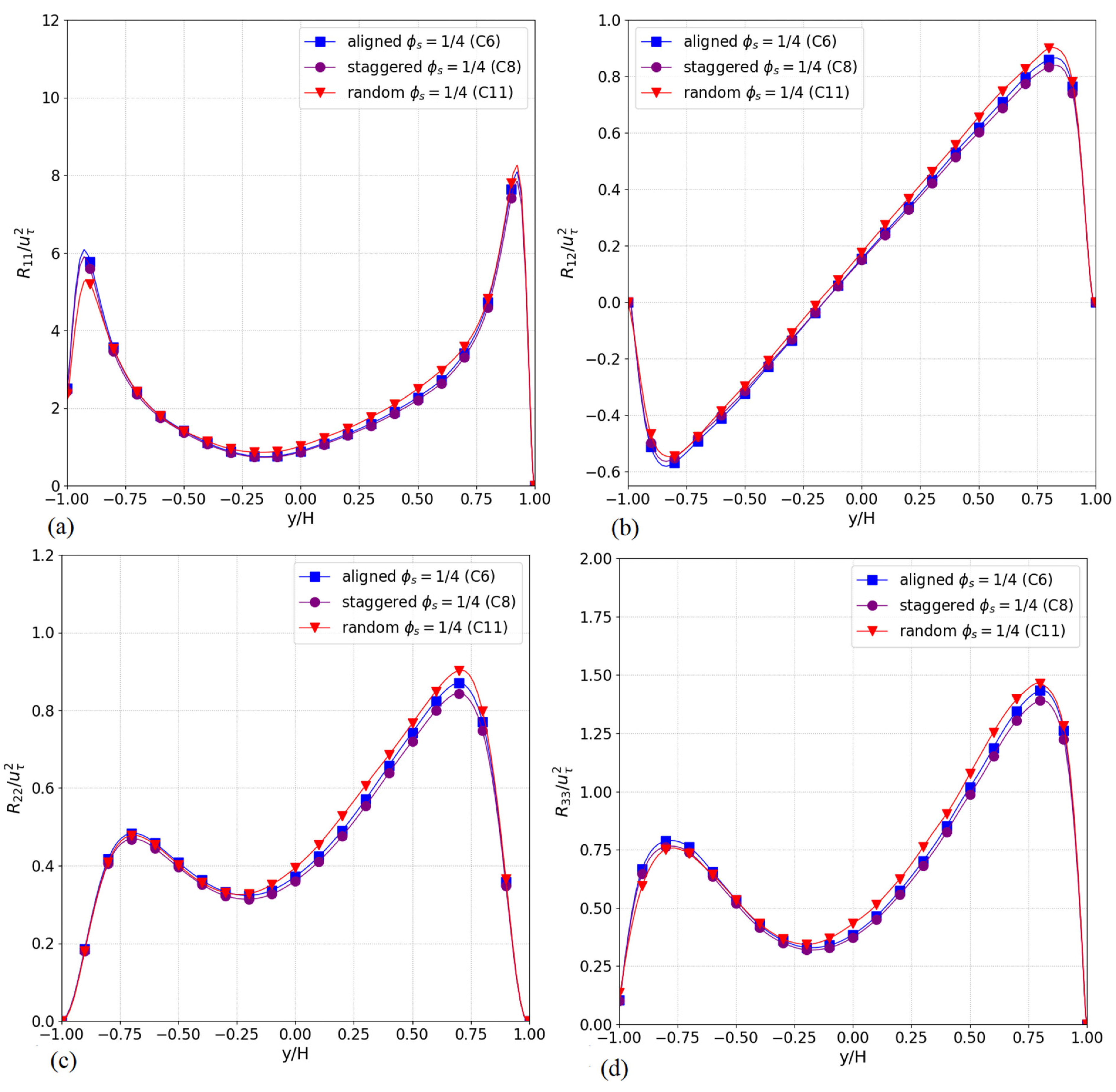
3.2. Reynolds Stresses
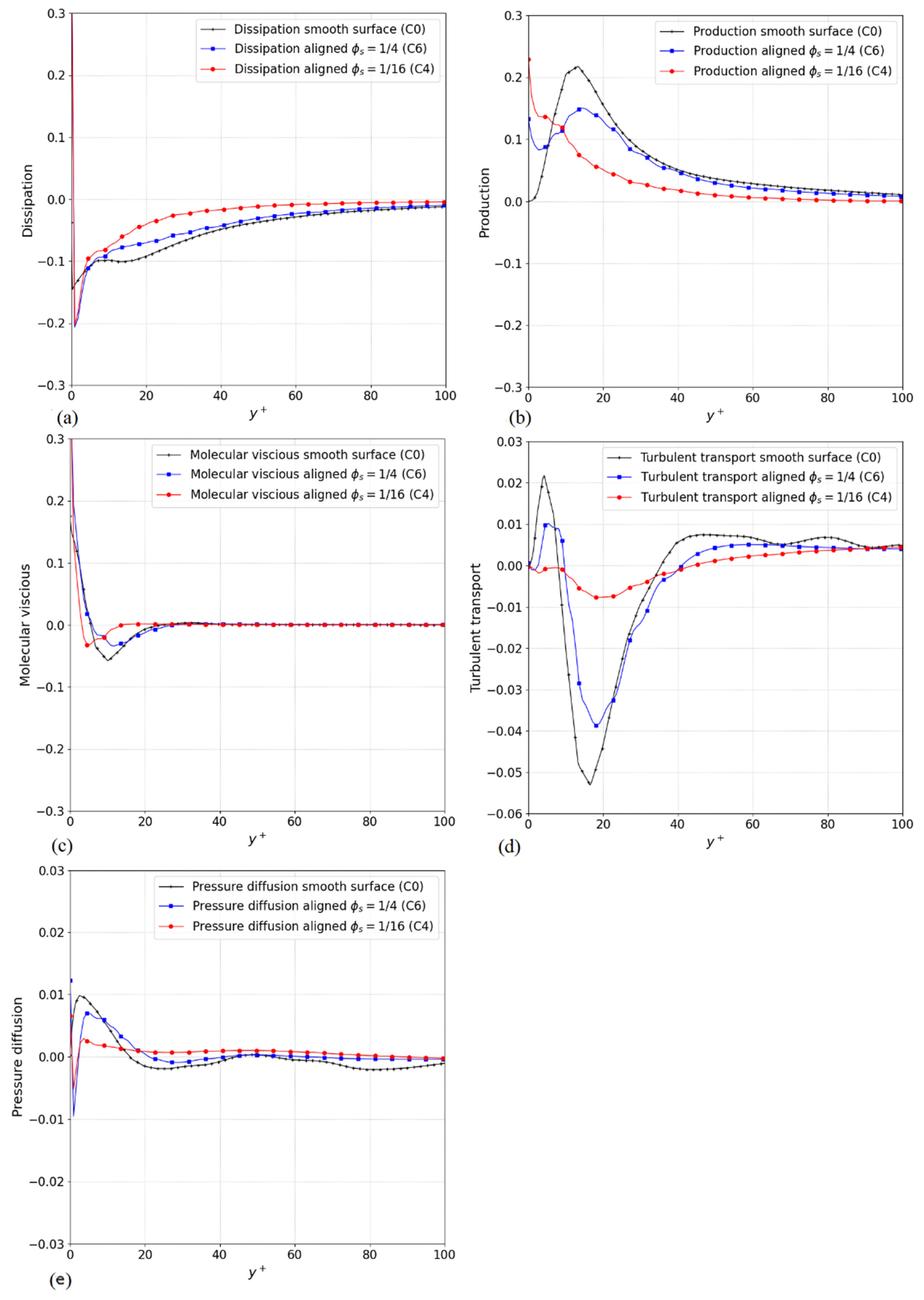
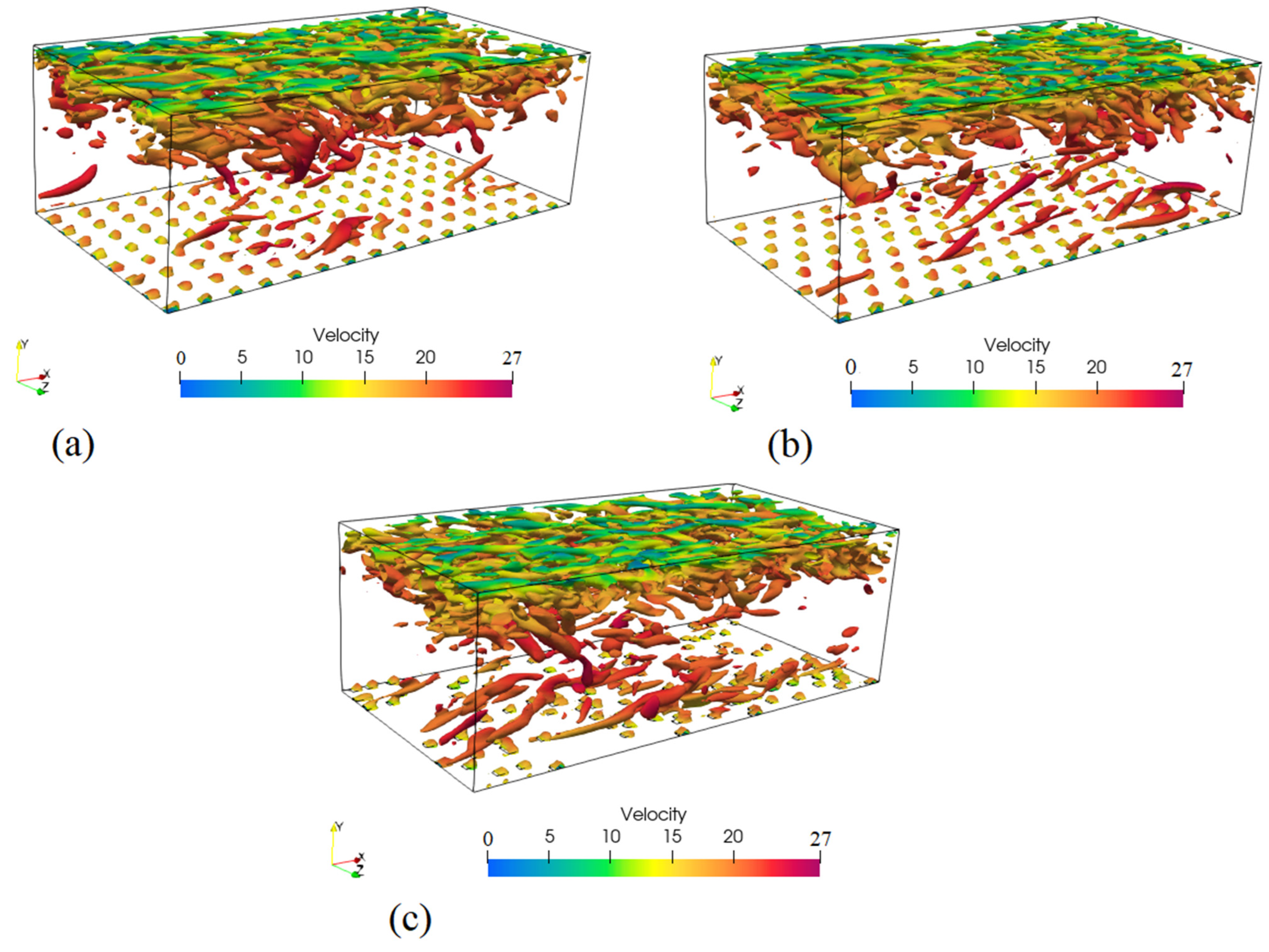
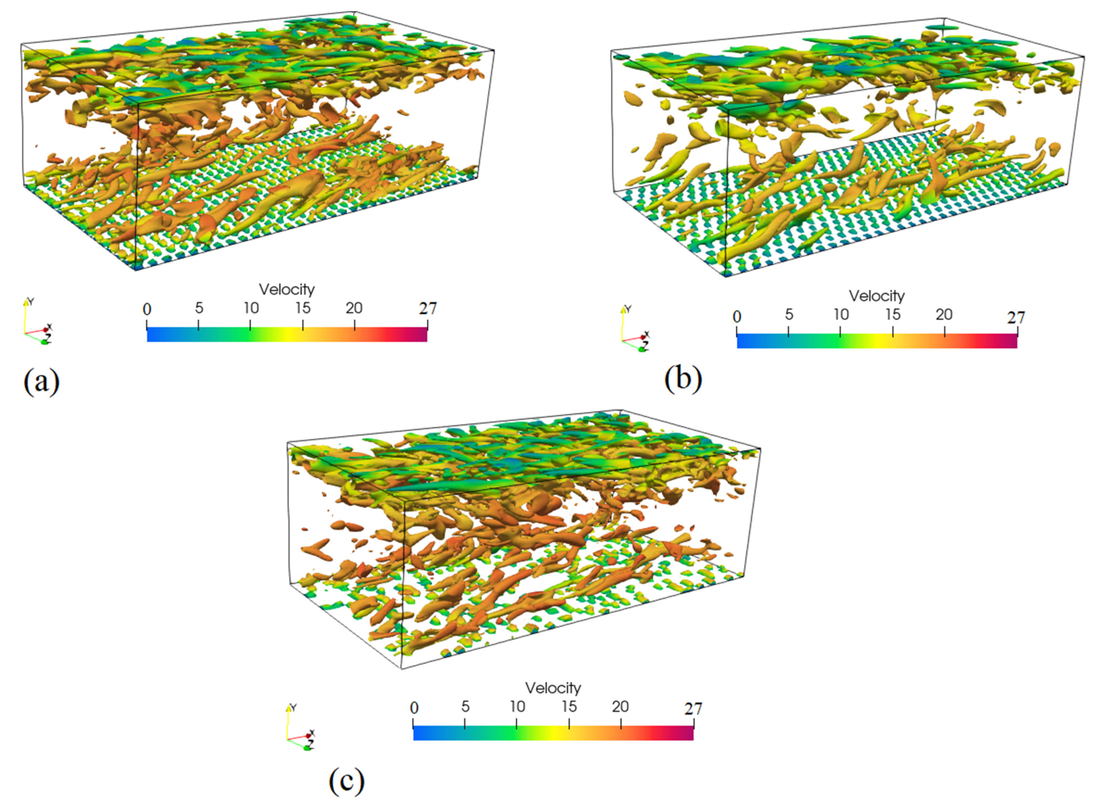
3.3. Turbulent Kinetic Energy(TKE) Budget and Flow Structures
4. Conclusions
Author Contributions
Funding
Institutional Review Board Statement
Informed Consent Statement
Data Availability Statement
Conflicts of Interest
Nomenclature
| Friction coefficient at the superhydrophobic surface | |
| Friction coefficient at the smooth wall | |
| Molecular diffusion | |
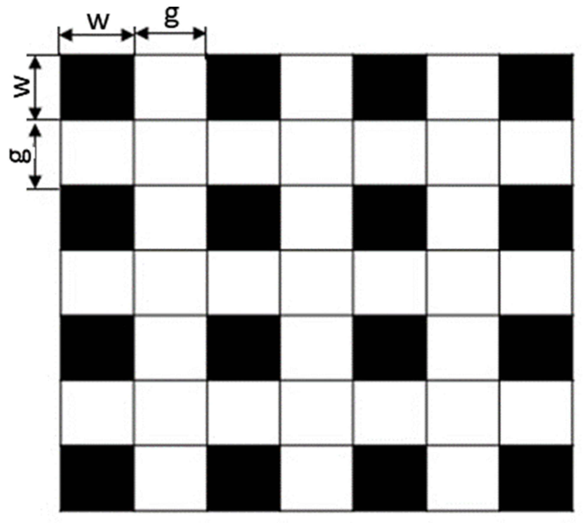
| g | Gap of superhydrophobic surface |
| H | Characteristic length (channel half-height). |
| Reynolds number based on friction velocity | |
| Bulk Reynolds number | |
| Production | |
| Turbulent diffusion | |
| Mean bulk velocity | |
| Slip velocity | |
| Dimensionless streamwise mean velocity | |
| Dimensionless streamwise mean velocity | |
| Friction velocity | |
| u+ | Near-wall velocity |
| Bottom wall friction velocity | |
| w | Width of superhydrophobic surface |
| Density of the fluid | |
| Top wall shear stress | |
| Bottom wall shear stress | |
| Wall shear | |
| Dissipation | |
| Solid fraction value | |
| Pressure diffusion | |
| Spanwise velocity |
Abbreviations
| CFD | Computational Fluid Dynamics |
| DNS | Direct numerical simulation |
| DR | Drag reduction |
| TKE | Turbulent kinetic energy |
| RANS | Reynolds averaged Navier Stokes equations |
| SHS | Superhydrophobic surface |
References
- Martell, M.B.; Rothstein, J.P.; Perot, J.B. An analysis of superhydrophobic turbulent drag reduction mechanisms using direct numerical simulation. Phys. Fluids 2010, 22, 065102. [Google Scholar] [CrossRef]
- Martell, M.B.; Perot, J.B.; Rothstein, J.P. Direct numerical simulations of turbulent flows over superhydrophobic surfaces. J. Fluid Mech. 2009, 620, 31–41. [Google Scholar] [CrossRef]
- Costantini, R.; Mollicone, J.-P.; Battista, F. Drag reduction induced by superhydrophobic surfaces in turbulent pipe flow. Phys. Fluids 2018, 30, 025102. [Google Scholar] [CrossRef]
- Ceccio, S.L. Friction Drag Reduction of External Flows with Bubble and Gas Injection. Annu. Rev. Fluid Mech. 2010, 42, 183–203. [Google Scholar] [CrossRef]
- Seo, J.; Mani, A. Effect of texture randomization on the slip and interfacial robustness in turbulent flows over superhydrophobic surfaces. Phys. Rev. Fluids 2018, 3, 044601. [Google Scholar] [CrossRef]
- Seo, J.; Garrcia-Mayoral, R.; Mani, A. Turbulent flow over superhydrophobic surfaces flow-induced capillary waves, and robustness of air-water interfaces. J. Fluid Mech. 2017, 835, 45. [Google Scholar] [CrossRef]
- Seo, J.; Mani, A. On the scaling of the slip velocity in turbulent flows over superhydrophobic surfaces. Phys. Fluids 2016, 28, 025110. [Google Scholar] [CrossRef]
- Busse, A.; Sandham, N. Influence of an anisotropic slip-length boundary condition on turbulent channel flow. Phys. Fluids 2012, 24, 055111. [Google Scholar] [CrossRef]
- Philip, J.R. Flows satisfying mixed no-slip and no-shear conditions. Z. Angew. Math. Phys. 1972, 23, 353. [Google Scholar] [CrossRef]
- Philip, J.R. Integral properties of flows satisfying mixed no-slip and no-shear conditions. Zeitschrift für angewandte Mathematik und Physik ZAMP 1972, 23, 960–968. [Google Scholar] [CrossRef]
- Lauga, E.; Brenner, M.P. Dynamic mechanisms for apparent slip on hydrophobic surfaces. Phys. Rev. E 2004, 70, 026311. [Google Scholar] [CrossRef]
- Im, H.J.; Lee, J.H. Comparison of superhydrophobic drag reduction between turbulent pipe and channel flows. Phys. Fluids 2017, 29, 095101. [Google Scholar] [CrossRef]
- Min, T.; Kim, J. Effects of hydrophobic surface on skin-friction drag. Phys. Fluids 2004, 16, L55–L58. [Google Scholar] [CrossRef]
- Fukagata, K.; Kasagi, N.; Koumoutsakos, P. A theoretical prediction of friction drag reduction in turbulent flow by superhydrophobic surfaces. Phys. Fluids 2006, 18, 051703. [Google Scholar] [CrossRef]
- Mori, E.; Quadrio, M.; Fukagata, K. Turbulent Drag Reduction by Uniform Blowing Over a Two-dimensional Roughness. Flow, Turbul. Combust. 2017, 99, 765–785. [Google Scholar] [CrossRef]
- Lee, M.; Moser, R.D. Direct numerical simulation of turbulent channel flow up to . Phys. Fluids 1999, 11, 943. [Google Scholar]
- Daniello, J.R.; Waterhouse, N.E.; Rothstein, J.P. Drag reduction in turbulent flows over superhydrophobic surfaces. Phys. Fluids 2009, 21, 085103. [Google Scholar] [CrossRef]
- Dainello, J.R. Drag Reduction in Turbulent Flows over Micropatterned Superhydrophobic Surfaces. Master’s Thesis, The University of Massachusetts Amherst, Amherst, MA, USA, 2009. [Google Scholar]
- Theobald, F.; Schäfer, K.; Yang, J.; Frohnapfel, B.; Stripf, M.; Forooghi, P.; Stroh, A. Comparison of Different Solvers and Geometry Representation Strategies for Dns of Rough Wall Channel Flow. In Proceedings of the 14th WCCM-ECCOMAS Congress 2020, Virtual Congress, 11–15 January 2021. [Google Scholar] [CrossRef]
- Issa, R.I. Solution of the implicit discretized fluid flow equations by operator-splitting. J. Comput. Phys. 1986, 62, 40. [Google Scholar]
- Jasak, H. Error Analysis and Estimation for the Finite Volume Method with Applications to Fluid Flow. Ph.D. Thesis, Imperial College of Science, Technology and Medicine, London, UK, 1996. [Google Scholar]
- Furzier, J.H.; Peric, M. Computational Methods for Fluid Dynamics; Springer: Berlin/Heidelberg, Germany, 2002. [Google Scholar]
- Ling, H.; Srinivasan, S.; Golovin, K.; McKinley, A.T.G.H.; Katz, J. Turbulent boundary layers in adverse pressure gradient. J. Fluid Mech. 2016, 801, 670. [Google Scholar]
- Smits, A.J.; McKeon, B.J.; Marusic, I. High–Reynolds number wall turbulence. Annu. Rev. Fluid Mech. 2011, 43, 353–375. [Google Scholar] [CrossRef]
- de Villiers, H. The Potential of Large Eddy Simulation for the Modelling of Wall Bounded Flow. Ph.D. Thesis, Imperial College of Science, University of London, London, UK, 2006. [Google Scholar]
- Abe, H.; Kawamura, H.; Matsuo, Y. Direct Numerical Simulation of a Fully Developed Turbulent Channel Flow With Respect to the Reynolds Number Dependence. J. Fluids Eng. 2001, 123, 382–393. [Google Scholar] [CrossRef]
- Bidkar, R.A.; Leblanc, L.; Kulkarni, A.J.; Bahadur, V.; Ceccio, S.L.; Perlin, M. Skin-friction drag reduction in the turbulent regime using random-textured hydrophobic surfaces. Phys. Fluids 2014, 26, 085108. [Google Scholar] [CrossRef]
- Srinivasan, S.; Kleingartner, J.A.; Gilbert, J.B.; Cohen, R.E.; Milne, A.J.B.; McKinley, G.H. Sustainable Drag Reduction in Turbulent Taylor-Couette Flows by Depositing Sprayable Superhydrophobic Surfaces. Phys. Rev. Lett. 2015, 114, 014501. [Google Scholar] [CrossRef]
- Rastegri, A.; Akhavan, R. The common mechanism of turbulent skin-friction drag reduction with superhydrophobic longitudinal microgrooves and riblets. J. Fluid Mech. 2018, 838, 104. [Google Scholar] [CrossRef]
- Hunt, J.C.R.; Wary, A.A.; Moin, P. Eddies, streams, and convergence zones in turbulent flows. In Proceeding of the Summer Program, Center for Turbulence Research, Stanford University; 1988; pp. 193–208. [Google Scholar]
- Wu, X.; Moin, P. Direct numerical simulation of turbulence in a nominally zero-pressure-gradient flat-plate boundary layer. J. Fluid Mech. 2009, 630, 5–41. [Google Scholar] [CrossRef]
- Adrian, J.R. Hairpin vortex organization in wall turbulence. Phys. Fluids 2007, 19, 041301. [Google Scholar] [CrossRef]
- Wedin, H.; Kerswell, R.R. Exact coherent structures in pipe flow: Travelling wave solutions. J. Fluid Mech. 2004, 508, 333–371. [Google Scholar] [CrossRef]
- Grant, H.L. The large eddies of turbulent motion. J. Fluid Mech. 1958, 4, 149–190. [Google Scholar] [CrossRef]
- Redford, J.A.; Sandham, N.D.; Roberts, G.T. Compressibility Effects on Boundary-Layer Transition Induced by an Isolated Roughness Element. AIAA J. 2010, 48, 2818–2830. [Google Scholar] [CrossRef]


| 180 | |
|---|---|
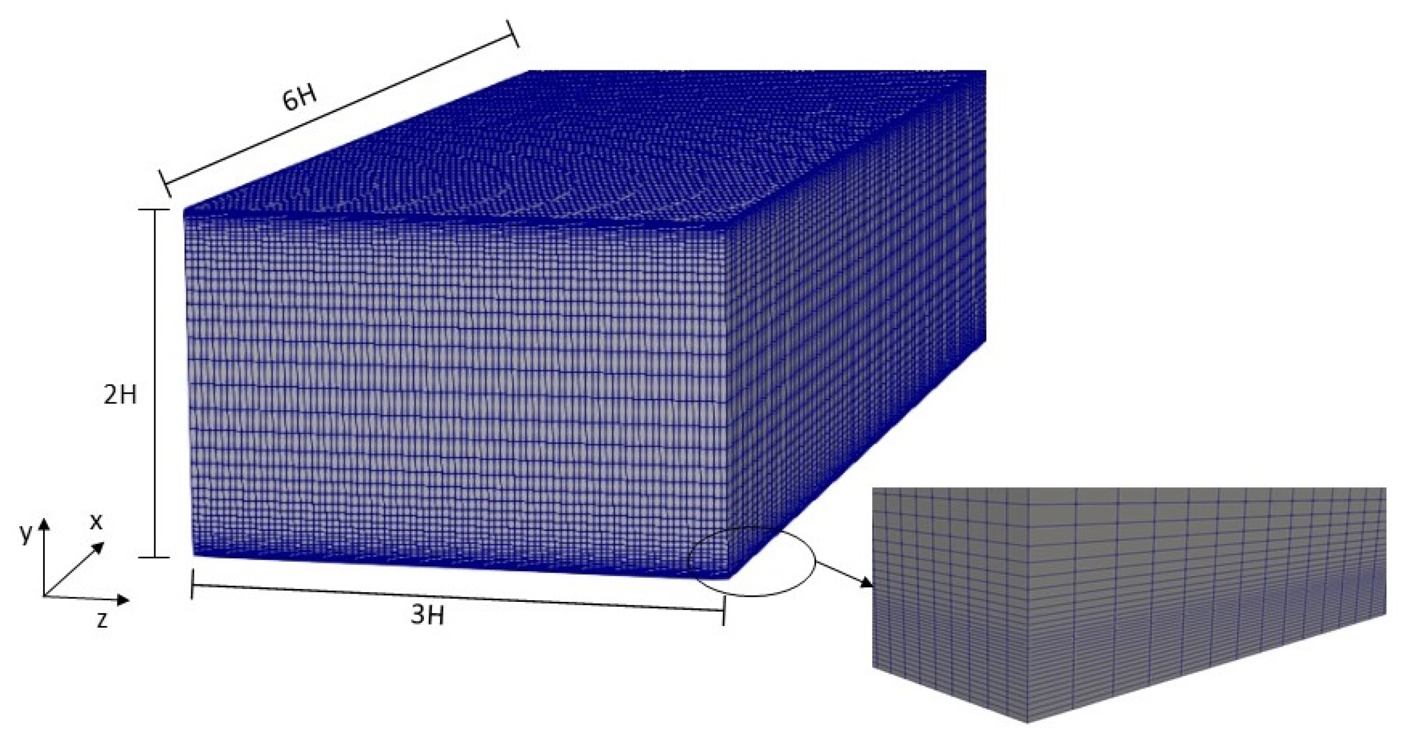
| Computational volume (x, y, z) | 6H × 2H × 3H |
| Grid number | 128 × 128 × 128 |
| Spatial resolution (∆x+,∆z+)) | 7.00, 5.0 |
| First wall-normal node height | 0.3 |
| Time-step size Um Mesh type CFL | 0.0001 15.72 Rectangular cuboid mesh 0.32 |
| Geometry | g/w | w/H | g/H | Name Case | |
|---|---|---|---|---|---|
| 180 | Smooth wall | - | - | - | C0 |
| ridge | 1.0 | 0.1875 | 0.1875 | C1 | |
| 1.6 | 0.14062 | 0.23436 | C2 | ||
| 3.0 | 0.09375 | 0.28124 | C3 | ||
| post | 3.0 | 0.09375 | 0.28124 | C4 |
| 180 | 15.72 | 18.38 | 1.17 | 5662 | 3309 | 295 | 8.11 × 10⁻³ |
| Geometry (Post) | ||||
|---|---|---|---|---|
| 180 | aligned | C4 | C5 | C6 |
| staggered | C7 | C8 | ||
| random | C9 | C10 | C11 |
| Case | C0 | C1 | C2 | C3 | C4 |
|---|---|---|---|---|---|
| DR (%) | - | 13.8 | 9.2 | 7.6 | 42.44 |
Publisher’s Note: MDPI stays neutral with regard to jurisdictional claims in published maps and institutional affiliations. |
© 2022 by the authors. Licensee MDPI, Basel, Switzerland. This article is an open access article distributed under the terms and conditions of the Creative Commons Attribution (CC BY) license (https://creativecommons.org/licenses/by/4.0/).
Share and Cite
Nguyen, H.T.; Chang, K.; Lee, S.-W.; Ryu, J.; Kim, M. Numerical Prediction of Turbulent Drag Reduction with Different Solid Fractions and Distribution Shapes over Superhydrophobic Surfaces. Energies 2022, 15, 6645. https://doi.org/10.3390/en15186645
Nguyen HT, Chang K, Lee S-W, Ryu J, Kim M. Numerical Prediction of Turbulent Drag Reduction with Different Solid Fractions and Distribution Shapes over Superhydrophobic Surfaces. Energies. 2022; 15(18):6645. https://doi.org/10.3390/en15186645
Chicago/Turabian StyleNguyen, Hoai Thanh, Kyoungsik Chang, Sang-Wook Lee, Jaiyoung Ryu, and Minjae Kim. 2022. "Numerical Prediction of Turbulent Drag Reduction with Different Solid Fractions and Distribution Shapes over Superhydrophobic Surfaces" Energies 15, no. 18: 6645. https://doi.org/10.3390/en15186645
APA StyleNguyen, H. T., Chang, K., Lee, S.-W., Ryu, J., & Kim, M. (2022). Numerical Prediction of Turbulent Drag Reduction with Different Solid Fractions and Distribution Shapes over Superhydrophobic Surfaces. Energies, 15(18), 6645. https://doi.org/10.3390/en15186645