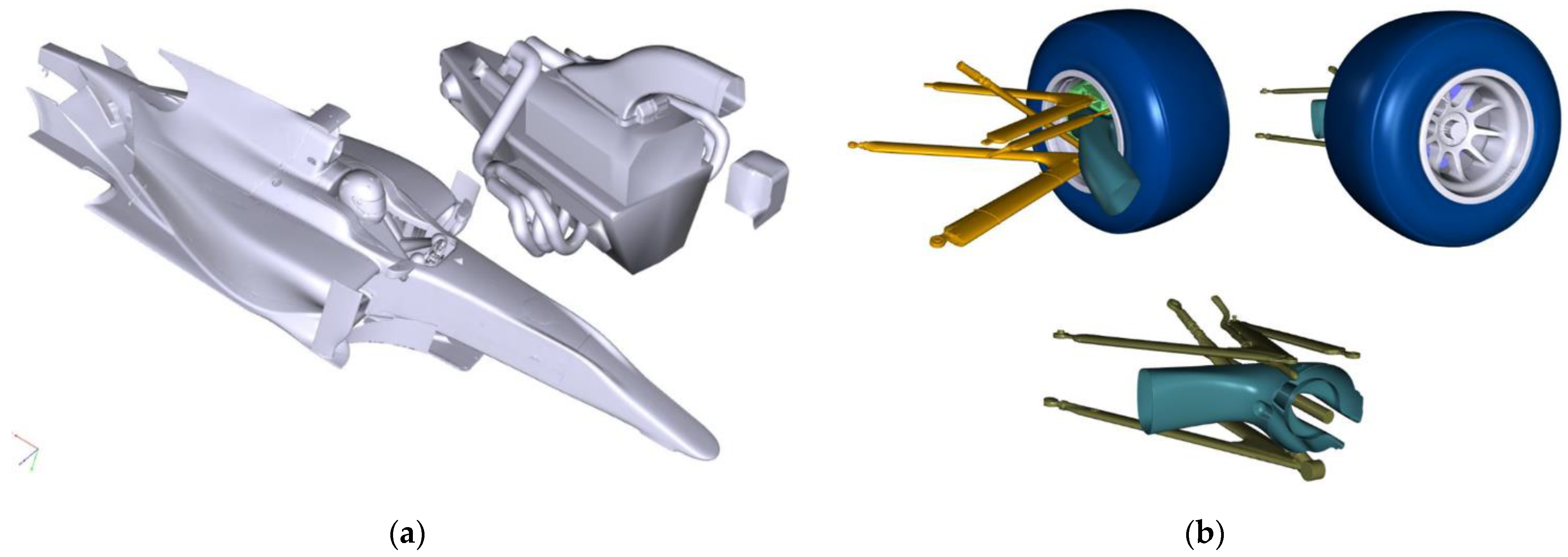
Article

Analyzing Porpoising on High Downforce Race Cars: Causes and Possible Setup Adjustments to Avoid It

Department of Mechanical and Industrial Engineering, University of Brescia, 25123 Brescia, Italy
*
Author to whom correspondence should be addressed.
Energies 2022, 15(18), 6677; https://doi.org/10.3390/en15186677
Submission received: 25 July 2022 / Revised: 12 August 2022 / Accepted: 6 September 2022 / Published: 13 September 2022

Abstract

:
The so-called porpoising is a well-known problem similar to bouncing that is affecting the dynamic behavior of basically all the field of 2022 Formula 1 racing cars. It is due to the extreme sensitivity of aerodynamic loads to ride height variations along a lap. Mid-way through the season race engineers are still struggling to cope with this phenomenon and its consequences, with regard to either physiological stress experienced by the drivers or to overall vehicle performance and stability. The paper introduces two kinds of models based on real-world chassis and aerodynamic data, where the above-mentioned downforce sensitivity has been arbitrarily recreated through the application of a decay function to aero maps. The first one is a quasi-static model, usually adopted as a trackside tool for controlling ride heights and aero balance, while the second, a fully dynamic model, recreates the interaction between oscillating aerodynamic loads and suspension dynamics resulting in a visible porpoising phenomenon. Basic setup changes have been tested, including significant static ride height variations. The paper should be seen as a proposal of guidelines in the search of a trade-off between aerodynamic stability and overall performance, without pretention of quantitative accuracy due to the highly confidential topic, which makes numerical validation impossible.

1. Introduction

The modelling of racing cars featuring high downforce levels, such as Formula 1 single-seaters and Le Mans prototypes, can offer a unique insight into the interaction between vehicle dynamics and aerodynamics. For 2022 the FIA—Fédération Internationale de l’Automobile—has modified the Formula 1 Technical Regulations completely. The change is mainly aimed at reducing downforce sensitivity to drafting (or slipstreaming) in order to make overtaking easier, thus forcing a complete changeover in terms of body shape and proportions as well as wing and underbody design. Most of the downforce is now produced by means of ground effect resulting from the presence of very large Venturi ducts built into the underbody. At the same time the peculiar shape of the 2022 front and rear wings, together with the absence of various winglets aimed at vortex generation or control, makes them less effective by far.
Start-of-season tests and the first races showed that such a one-off event is somehow a leap into the unknown: more or less all cars are suffering from severe bouncing—the so-called porpoising—along the straights. This is caused by aerodynamic instability, and can result in floor damage, driver discomfort, discontinuous tire contact patch loading, and poor high-speed performance overall. As a matter of fact, the problem was first experienced with ground-effect Formula 1 cars about 45 years ago: it is due to marked non linearities of the downforce along ride height variation induced by downforce itself. In simple words the air flow under the car stalls whenever the floor is very close to the ground, i.e., at high speed. Downforce collapses and the car bounces back to static ride heights (or even beyond), restoring downforce in turn as a consequence. Nearly half-way through the season the problem is still there, with drivers beginning to complain about potential consequences in terms of spine injuries.
Aerodynamic characteristics of Formula 1 cars are considered highly confidential and therefore they are not usually available to the vehicle dynamics community, even more so for newly designed cars of the 2022 season, where underbody aero is said to be dominated by vortex flow. Nevertheless, the porpoising phenomenon can be studied by means of a model built on the basis of a similar car with ground-effect aerodynamics, as what really counts here is ride height sensitivity.
The authors have used a lumped element model for simulating coupling between non-linear aerodynamics and suspension dynamics in [1]. The present study however describes a methodology typically aimed at performance improvements through optimization of aerodynamics and mechanical setup by means of more accurate models. This simulation approach is often used for trackside engineering [2] and for off-line lap time simulations as well [3,4,5,6,7,8,9]. Other potential applications are aimed at the design of peculiar suspension and steering systems [10,11] and advanced powertrains [12], while lap time simulation can also be addressed at the evaluation of physiological parameters when driving at the limit [13]. Lap time simulation is also used quite often for autonomous race car control [14,15] and tire performance optimization [16], and also to consider the variation of tire functional characteristics along the lap [17].
A model of a single-seater GP2/Formula 2 racing car, conceptually similar to a Formula 1, has been created for the purpose. Although featuring just four DOF and being quasi-static, the model is highly detailed. The suspension model for instance is based on suspension kinematics computation by means of a dedicated software tool described in [18,19] and provides for variable motion ratio, pressurized gas damper preload, non-linear rubber bump stops and it is coupled with a variable radius tire model taking vertical force, vehicle speed, and wheel camber angle into account. Both models are based on official information and data supplied by the vehicle and tire manufacturers respectively.
A more sophisticated approach has been adopted for numerical modelling of the aerodynamics characteristics, featuring strong non-linearities that make modern racing cars highly ride height- and pitch-sensitive. 3D scanning has been performed on a real-world GP2 racing car with the aim of recreating a complete CAD model of the car body surfaces, comprehensive of outboard wheel/tire assemblies, front and rear wings, various winglets, driver’s helmet, and underbody floor with Venturi ducts. The CAD model has been used for a comprehensive CFD study aimed at estimating the so-called aerodynamic maps (or aero maps) i.e., drag, downforce, and aero balance characteristics with reference to underfloor distance from the road surface along the front and rear axles. Discussions on aerodynamic properties of current F1 cars and on the CFD analysis itself go beyond the scope of this paper, which is focused instead on the effect of ride height sensitivity on vehicle dynamics.
After a thorough comparison with original data supplied by the vehicle manufacturer for validation, the aero maps have been applied to the four DOF model to obtain quasi-static, speed-dependent ride height variations, suspension stiffness at ground, overall downforce, and its fore/aft distribution, commonly referred to as aero balance.
In order to simulate porpoising, a modification of the aero maps has been implemented by introducing further ride height sensitivity in an attempt to replicate the aerodynamic instability of the 2022 Formula 1 cars. The same aero maps—either original or modified—have been applied to a full vehicle dynamics model built within the VI-grade environment. These simulations allow for the reproduction and analysis of the porpoising phenomenon with its peculiar dynamic characteristics that trigger aerodynamic instability by interacting with the suspension system. Some attempts have been made to reduce or remove porpoising through variation of typical setup parameters like damping, spring stiffness, bump stop gaps and stiffness, and static ride heights.
Finally complete lap time simulations were carried out in order to compare the behavior of the original model with the same car affected by porpoising and with the latter car with modified static ride heights, in an attempt to identify effective solutions to the problem in terms of overall vehicle performance.

2. Materials and Methods

Since a CAD model was not available to teams, a real-world GP2 car was 3D scanned, including driver helmet, underbody, sidepod internals (basically water radiators and exhaust), engine inlet/airbox, suspension arms, and wheel assemblies with brake ducts. The car was artificially loaded in order to scan the tires with a certain level of deflection. Scan data were then processed into a digital surface model in STEP format suitable for CFD analysis, see Figure 1 and Figure 2.
A GP2/Formula 2 single-seater is a professional racing car providing full adjustability in terms of either mechanical setup (basically several suspension and steering settings, gearbox ratios, limited-slip differential) and aerodynamics, where front and rear wings can be adapted to suit circuit geometry, weather conditions and driver style, physiology, and habits. The rear wing type (mono- or bi-plane) and settings mainly define the overall level of downforce and drag, while the front flap settings mainly define the aero balance, see Figure 2b.
Add-on devices like the so-called Gurney flaps (or nolders) can also be fitted on the trailing edge of both the front and rear flaps. On top of that, the car features large underbody Venturi ducts therefore it can be defined as a ground-effect car, whose behavior and performance are not so far away from a modern Formula 1 car. As such aerodynamic actions are extremely sensitive to ride height and pitch angle, they are defined through the distances of the underbody reference plane from the ground in correspondence of both the front and rear axles: the Front Ride Height (FRH) and Rear Ride Height (RRH) respectively.
Prior to CFD analysis some assumptions were made with regard to car settings and other details. An aerodynamic baseline setup in terms of front and rear wing configuration and static ride heights was defined on the basis of the authors’ experience as trackside engineers, namely referring to a qualifying configuration for the Sakhir international circuit in Bahrain. On top of that radiator characteristics as well as the exhaust gas flow rate were also defined.
The overall aerodynamic performance of a racing car can be identified through the set of functional parameters:
X = C D , C Z , A B ,
where CD is the drag or resistance coefficient, CZ is the coefficient of downforce generated by aerodynamic devices built into the vehicle body such as wings and undertray, and AB is the above-mentioned aero balance i.e., the fore/aft distribution of downforce expressed as percentage on the front axle.
The open-source software OpenFOAM was used to perform a CFD analysis of the whole car in co-operation with the British company TotalSim. While some preliminary runs enabled fine tuning of the mesh and identification of critical areas where flow is detached from the body surface, various runs where required to sweep through the front and rear ride height range, starting from setup values all the way down to hitting the ground with the underbody. Setup or static ride heights are defined at zero speed: FRHS and RRHS.
As stated before, an in-depth description of the meshing and CFD stages is beyond the scope of this paper, as are detailed analysis of flow dynamics, boundary layer, vortex structure, and pressure fields around the car. Nevertheless, Figure 3, Figure 4 and Figure 5 show examples of some post-processing methods made available by CFD analysis.
What is relevant here is that such a sweep enabled generation of the so-called aerodynamic maps, therefore replacing experimental testing in the wind tunnel. These 2D look-up tables describe the functional properties of the car in terms of aerodynamic performance. They feature values of the products CDS, CZS, as well as aero balance AB, as a function of the combination of dynamic front and rear ride heights, FRH and RRH respectively. S is the frontal area of the car, often assumed as a nominal value of one meter squared for a single-seater racing car.
Figure 6, Figure 7 and Figure 8 show the CDS, CZS, and AB aero maps for the aerodynamic configuration under scrutiny.
Interpolation of aerodynamic maps can be performed in many different ways: from ANN (Artificial Neural Networks) to the Kriging regression method to Akima splines [20,21,22,23,24]. A common approach based on [25] is a polynomial function of the type:
X = a 1 · F R H 3 + a 2 · R R H 3 + a 3 · F R H 2 · R R H + a 4 · F R H · R R H 2 + a 5 · F R H 2 + a 6 · R R H 2 + a 7 · F R H · R R H + a 8 · F R H + a 9 · R R H + a 10   ,
where a set of coefficients a1a10 can be computed by means of a regression technique for each of the three functional parameters CDS, CZS, and AB.
The effect of setup changes in terms of wing angle is computed as a contribution to be added to the baseline output from the look-up tables for each wing profile (mainplane and/or flaps):
Δ X = b 1 · α 2 + b 2 · α + b 3 + c ,
where a is the angle of attack, b1, b2 are the related coefficients and c is the further contribution of any add-ons. This formula is not suitable for modeling the stall phenomenon often occurring for large values of a, which should be avoided anyway.
Overall drag FD and downforce FZ can then be computed for any aerodynamic setup and for any combination of front and rear ride heights by means of the well-known expressions:
F D = 1 2 ρ C D S V 2 ,
F Z = 1 2 ρ C Z S V 2 ,
where r is the air density and V is the vehicle speed. Downforce on the front axle FZfrt and rear axle FZrr can be respectively computed as:
F Z f r t = F Z · A B ,
F Z r r = F Z · ( 1 A B )   .
While aerodynamic efficiency is computed as the ratio between downforce and drag as usual:
E f f = F Z F D   .
The peculiar shape of the efficiency map—which is obviously a function of front and rear ride heights too—is emphasized in Figure 9.
These functional characteristics have a massive impact on tire vertical loads, and hence on racecar drivability, performance, and ultimately lap time. Especially aero balance is of particular interest for the trackside engineer: even apparently small changes can affect cornering balance in terms of understeer/oversteer and vehicle stability, especially in the turn-in transient phase. According to the authors’ experience a 0.2% aero balance variation can be easily perceived, at least by a professional driver.
All the three aerodynamic parameters are therefore non-linear functions of dynamic ride heights:
X = F D , F Z , A B = f ( F R H , R R H )   ,
Dynamic ride heights are in turn a function of static ride heights, overall downforce, and aero balance, hence they are strongly dependent on vehicle speed on one side, and on parameters related to chassis settings, such as tire and suspension stiffness at ground level, on the other side.
The above Figure 6, Figure 7, Figure 8 and Figure 9 show that downforce tends to increase dramatically when the car gets closer to the ground, especially at the front end, thus moving the aero balance forward with increasing speed. It is therefore mandatory for the trackside engineer to master the interaction between aerodynamics and mechanical setup by means of proper simulation tools.

2.1. Quasi-Static and Full Vehicle Models

A comprehensive vehicle model is therefore required, where speed and static ride heights are the input variables, parameters defining aerodynamic items and chassis setup in terms of overall vertical stiffness enter the equation, and aerodynamic actions result in the computation of dynamic ride heights, contact patch forces, and aero balance as a function of speed. A typical tool for trackside vehicle management responding to the above requirements is the well-known quasi-static, four DOF vehicle model taking heave and pitch as well as front and rear tire radial deflections into account.
Suspension stiffness at ground is mainly a function of suspension kinematics and spring stiffness, the latter being either a traditional coil spring or a torsion bar, as it is the case of the GP2 front axle. Pressurized dampers—a standard in motorsport—play a role as well: the gas preload PG is set by the pressure in the floating chamber and by the geometry of the damper piston and shaft. It can be around 400–500 N or even more hence its effect is not negligible.
The spring preload PS should be taken into account as well if some form of rebound stop is present. The overall spring rate is therefore
K S p r i n g = { i f   F S p r i n g ( P S + P G ) K S p r i n g i f   F S p r i n g > ( P S + P G ) } ,
where KSpring and FSpring are the stiffness and force of the coil spring alone. A linear spring stiffness however is not suitable for the requirements of a high-downforce, ride-height-sensitive racing car with strongly non-linear aero maps. The spring-damper unit therefore is usually complemented by a “progressive” bump stop working in parallel with the spring. The force vs. deflection curve of a typical rubber bump stop can be described by means of a fourth-order polynomial going through the coordinate origin, see Figure 10. As such it is defined by a set of coefficients e1e4 and comes into play once a free gap d is covered by the spring deflection D. The overall springing force is therefore
F S p r i n g = { K S p r i n g · D i f   D d K S p r i n g · D + e 1 ( D d ) + e 2 ( D d ) 2 + e 3 ( D d ) 3 + e 4 ( D d ) 4 i f   D > d } ,
where the gap d can also be set to a negative value.
Suspension kinematics can be considered by means of the so-called Motion Ratio MR, to be defined as
M R = d W d D = f ( W )
where W is the wheel displacement and D is the corresponding spring deflection, or the equivalent linear deflection of the torsion bar. Being a function of wheel displacement, the Motion Ratio is directly related to ride height for each axle. In the case of a GP2 car however MR(W) is nearly linear, and in addition to the limited suspension travel typically used on a racecar, it can be assumed to be a constant value MR0 linearized around the setup ride height. The overall force at the wheel is therefore [26]:
F W h e e l = 1 M R 0 · F S p r i n g .
Additional items like the so-called third element can be added with their own, linear or non-linear stiffness and motion ratio. Tire radial stiffness characteristics play a major role hence they must be considered. The tires do not only act as a spring in series with the suspension: they are subjected to growth due to centrifugal force as well. Camber angle g and eventually cornering forces FY also affect tire radius. According to refs. [27,28] the tire loaded radius can be computed by means of the empirical expressions:
R = R 0 d R ,
d R = F W h e e l t 1 · I P + t 2 · V 2 + t 3 · V + t 4 + t 5 · | γ | + t 6 · F Y 2 / F W h e e l + t 7 · V 2 + t 8 · V ,
where R is the tire loaded radius under dynamic conditions, R0 is the nominal tire radius in static conditions, and dR is the radial deflection, IP is the inflation pressure, V is the vehicle speed, and finally t1…t8 are a set of coefficients describing dimensional tire properties under vertical load for a certain speed, to be determined (usually by the tire manufacturer) on a dedicated test bench. Front and rear tires feature different dimensions and a specific structure hence two sets of coefficients are required for a single-seater racing car.
The overall springing rate at contact patch level is therefore strongly non-linear and “progressive”: it is mainly a function of suspension jounce and vehicle speed among other variables. It requires careful design on both axles in order to keep pitch angle hence aero balance under control with increasing speed, while avoiding bottoming at high speed and on road surface irregularities. Most of all, it means that static ride heights and setup parameters affecting springing rates front and rear are all powerful tools for setup adjustment, car balance optimization and finally for performance improvement.
Typical output graphs are displayed in the following images (Figure 11, Figure 12 and Figure 13) and explained in the captions.
The quasi-static, four DOF model described above was thoroughly developed and validated across four years of race engineering activity at international level, via comparison with on-board data acquisition and with the help of subjective feedback from professional drivers, especially with regard to the aero balance, which is one of the key parameters for overall performance. More recently, a full vehicle model was built from scratch in the VI-grade simulation environment and compared to the four DOF model for validation, following the very same approach for modeling suspension and aerodynamics in particular. All the various non-linearities were thus taken into account, including the ride-height-sensitive aero maps. Suspension kinematics for instance was fully modelled by means of a proprietary design tool [18] and included non-linearities like variable motion ratio and progressive bump stops. An official .tir file-based tire model was used as supplied by the tire manufacturer, for loaded radius and radial stiffness properties and for in-plane lateral and longitudinal forces, governing handling, acceleration, and braking. The vehicle model was then tested in steady-state mode with increasing longitudinal speed along a straight line and around a Formula 1 circuit like Sakhir in Bahrain, in order to check for model robustness and lap time accountability, although without claiming full correspondence between the GP2 car model and a highly performant, modern Formula 1 car complying with new technical regulations for the 2022 season. This model is referred to as Setup #1 later in the text.

2.2. Triggering the Porpoising Phenomenon

Different types of arbitrary decay functions were applied to the original aero maps and tested in order to reproduce the peculiar bouncing dynamics due to extreme sensitivity of downforce to front and rear ride heights from the ground: the infamous porpoising, as Formula 1 drivers, technical staff, and journalists have named it. The following function was chosen according to the criteria listed ahead, where FZfrt_Porp for instance is the front portion of downforce modified by means of the arbitrary decay curve:
F Z f r t _ P o r p ( F R H ) = F Z f r t · ( F R H F R H S ) ( 1 d ) ,
so that in static conditions:
F Z f r t _ P o r p ( F R H S ) = F Z f r t ( F R H S ) ,
and whenever the underbody panel is in contact with the ground:
F Z f r t _ P o r p ( 0 ) = 0 ,
while similar decay function is applied to the rear downforce:
F Z r r _ P o r p ( R R H ) = F Z r r · ( R R H R R H S ) ( 1 d ) .
Parameter d was set to a value of 7 in order to represent an abrupt loss of downforce whenever the underfloor drops all the way down to the ground. Figure 14 and Figure 15 show the above decay functions for front and rear downforce and the effect on ride heights as a function of vehicle speed as computed in the four DOF model i.e., statically, as well as on aero balance and efficiency. Because of the decay function, downforce is abruptly reduced once the car underfloor gets very close to the ground at high speed, resulting in turn in higher ride heights as well as heavily modified aero balance and efficiency curves. In steady state the aero balance trend appears more consistent, while efficiency is reduced at high speed.
Once the decay functions are also applied to the full vehicle model, the effect is clearly visible and appears quite similar to porpoising, recalling what happens on current Formula 1 cars. Figure 16, Figure 17 and Figure 18 show a comparison between the baseline GP2 car model with original aero maps (Setup #1, in blue) and the model with decay functions applied to aero maps (referred to as Setup #2, in red) in terms of straight-line behavior with increasing speed. What appears a simple effect when observed in quasi-static mode turns into a complex, cyclical combination of axle jounce and body pitch, where axle jounce is in turn a combination of damped suspension jounce and underdamped oscillation on tires. Validation with a real-world case unfortunately is not possible because Formula 1 vehicle data recorded on-board are not available outside the teams themselves, nevertheless a reference for the typical porpoising frequency can be easily estimated with the help of many videos available on the web by simply counting the number of bouncing cycles in a time interval, while a reference for the amplitude of vertical acceleration oscillations is available on [29]. Both numbers are extremely similar to what was achieved with the full vehicle model; hence we can say that porpoising is reproduced in a reasonably correct way.
It can also be stated that a vertical oscillation frequency around 6 Hz (see Figure 15) falls in a range where tolerability for the human body is low [30,31]. This is basically confirmed by various F1 drivers actually complaining of extreme discomfort, fatigue, loss of driving focus, and potential neck and spine injuries.

3. Results

Availability of the full model together with its capability for approximating the porpoising phenomenon makes it possible to search for a trial solution, although within the domain of the so-called mechanical setup only, since changes in terms of aerodynamics are certainly outside the scope of this paper. Given the intrinsically dynamic nature of porpoising, the very first variable that appears as a potential improvement is damping: front and rear damper curves were therefore modified separately, just by multiplying damping force values by two. Needless to say, in the real world such a massive change would imply detrimental effects in other areas of vehicle behavior—riding on kerbs for instance—but these consequences can be neglected at this modeling stage; in any case both changes were effective to a certain extent only. For the sake of simplicity Figure 19 and Figure 20 show the results for front bumping modification only, as rear damping returns a very similar trend.
The reason is that porpoising dynamics are basically caused by underdamped tire deflection, as shown above in Figure 18. In other words, hydraulic dampers cannot provide enough damping in the system to control body oscillations.
A second, straightforward attempt was an increased rubber bump stop stiffness, meaning in turn an overall larger wheel rate once the bump stop gap has been covered by suspension jounce. This change was tried at the rear only, as porpoising seems to be triggered by the rear axle or at least it seems to start there. Figure 21, Figure 22 and Figure 23 show however that the effect is not in terms of system dynamics but only in terms of downforce-related dynamic ride heights: porpoising is basically delayed until a higher vehicle speed is reached simply because the dynamic ride heights are higher. A change in bump stop characteristics can be seen therefore as a tuning item, but not as a solution. Similar results were achieved by increasing spring stiffness or by changing the gap d.

The Effect of Static Ride Height Variations

All the above seems to suggest that a significant improvement can be achieved by increasing the static ride heights, in turn affecting dynamic ride heights as well. At first a variation was tried separately on the two axles. The front was raised by 10 mm, which is quite a change for a ground effect car. Bouncing amplitude is reduced significantly at the front, and the rear also benefits from the change (see Figure 24), although average downforce is also reduced.
The rear end was raised by 20 mm instead. In this case the effect on the rear axle is significant as bouncing is nearly removed. The front end also benefits significantly (Figure 25).
Now in order to achieve a similar aero balance in the medium speed range, at least in quasi-static conditions, a 1:2 proportion between front and rear variations in terms of ride height is required. The next step is therefore the following variation: FRHS +5 mm, RRHS +10 mm, referred to as Setup #3. This time the result is satisfactory: the onset of porpoising is delayed until 260 kph, and the average downforce is higher, see Figure 26 and Figure 27.
A second attempt with the following variation relative to the baseline setup: FRHS +10 mm, RRHS +20 mm, referred to as Setup #4, was finally successful in removing porpoising completely, although at the expense of overall downforce and efficiency. Figure 28, Figure 29 and Figure 30 compare the latter configuration with the baseline and the baseline with decay functions.

4. Discussion

Full lap time simulations were then performed in the VI-grade software environment in the search for a reasonable tradeoff between vehicle performance and aerodynamic stability, in other words for assessing the impact of static ride height variations on outright lap time. The virtual driver adopted for the simulation is based on MaxPerformance, a proprietary algorithm for vehicle control during closed-loop driving maneuvers developed by VI-grade and tuned according to the authors’ experience.
The comparison was carried out taking the Sakhir circuit in Bahrain (Figure 31) as a reference because of its nature of combined slow, medium- and high-speed corners, making it representative of a vast selection of Formula 1 circuits. Table 1 shows the configurations tested, each with the related lap time.
The standard vehicle configuration with baseline Setup #1 was tuned with real-world data. Such a process is not within the scope of this paper hence it is not dealt with here, in any case the final difference with the real car in terms of lap time is negligible (+0.8%) hence this model can be considered validated and capable of a 3rd or 4th position overall in the 2013 Qualifying session in Bahrain [32].
For the sake of clarity, it should also be stated that the other configurations were not fine-tuned after the modifications, in order to avoid the introduction of additional variables in the loop. The setup configuration with decay functions #2 is much slower than the baseline and would qualify in 22nd position. Massive porpoising appears along all the straights, see Figure 32. It is worth noting that the amplitude of oscillations at the rear axle is even larger than the “normal” amplitude of suspension jounce due to downforce, while the front end appears less prone to aerodynamic instability. The average downforce is reduced accordingly, while vertical acceleration levels at the center of gravity exceed 1.5 g, making them a severe hazard for the driver’s body (see Figure 33).
Configuration #4 with static ride height variations FRHS +10 mm, RRHS +20 mm is capable of removing porpoising completely, although at the expense of downforce. As a matter of fact, such a car would qualify in 20th position in 2013. Configuration #3 with static ride height variations FRHS +5 mm, RRHS +10 mm is finally a reasonable tradeoff: porpoising appears only at the end of the straight i.e., at top speed (see Figure 34), while the amplitude of vertical accelerations experienced by the driver is reduced to 0.8 g and just for a few seconds, resulting into an appreciable improvement in terms of comfort. On top of that lap time would be good for a 16th position in the 2013 starting grid, and this improvement is largely due to fairly consistent downforce levels (see Figure 35).
The above improvement is even clearer in Figure 36, where configurations #2 (with decay functions/porpoising) and #3 (FRHS +5 mm, RRHS +10 mm) are compared directly.

5. Conclusions

Insiders and professionals in the motorsport world know very well that the so-called porpoising, which is heavily affecting the dynamic behavior of 2022 Formula 1 racing cars, is very difficult to deal with both for the drivers (complaining about back and neck pain and increased physiological stress during grand prix races) and for the race engineers trying to maximize vehicle performance. Mid-way through the season all the teams are still struggling with this problem, caused by extreme sensitivity of aerodynamic loads to dynamic ride heights. The paper presents two kinds of models where such an aerodynamic sensitivity has been arbitrarily recreated: a quasi-static model, usually adopted as a trackside tool for controlling ride heights and aero balance, and a fully dynamic model, where the interaction between oscillating aerodynamic loads and suspension dynamics results in the porpoising phenomenon.
Basic setup changes have been tested on the second model, resulting in no or limited benefits. Only a significant increase of static ride heights proves resolutive as it can delay or remove porpoising, although at the expense of downforce levels hence performance, in accordance with typical statements often issued by Formula 1 teams. Finally lap time simulations have been carried out with the aim of assessing such a performance loss and to offer guidelines in the search of a tradeoff between aerodynamic stability and overall performance.
Future work will be about transferring the model to the real-time environment for DIL (Driver-In-the-Loop) testing on a professional driving simulation, with the aim of taking subjective aspects into account. The effect of properly tuned devices like a mass damper and an inerter on porpoising will be investigated as well, regardless of the fact that they are both forbidden by the current Technical Regulations issued by the Formula 1 governing body, the FIA.

Author Contributions

Conceptualization, M.G.; Data curation, D.C. and P.M.; Funding acquisition, D.C.; Investigation, D.C.; Methodology, M.G. and D.C.; Supervision, M.G.; Validation, P.M.; Visualization, G.S.; Writing—original draft, M.G.; Writing—review & editing, G.S. All authors have read and agreed to the published version of the manuscript.

Funding

This research received no external funding.

Institutional Review Board Statement

Not applicable.

Informed Consent Statement

Not applicable.

Data Availability Statement

Not applicable.

Acknowledgments

The authors would like to thank Dallara Automobili S.p.a.

Conflicts of Interest

The authors declare no conflict of interest.

References

  1. Marchesin, F.P.; Barbosa, R.S.; Gadola, M.; Chindamo, D. High downforce racecar vertical dynamics: Aerodynamic index. Veh. Syst. Dyn. 2018, 56, 1269–1288. [Google Scholar] [CrossRef]
  2. Marchesin, F.P.; Barbosa, R.S.; Gadola, M.; Chindamo, D. A road-holding index based on ride dynamics for high-downforce racing cars. IOP Conf. Ser. Mater. Sci. Eng. 2019, 538, 12069. [Google Scholar] [CrossRef]
  3. Dal Bianco, N.; Lot, R.; Gadola, M. Minimum time optimal control of a GP2 race car. Proc. Inst. Mech. Eng. Part D J. Automob. Eng. 2018, 232, 1180–1195. [Google Scholar] [CrossRef]
  4. Chindamo, D.; Gadola, M.; Bonera, E.; Magri, P. Sensitivity of Racing Tire Sliding Energy to Major Setup Changes: An Estimate Based on Standard Sensors. Energies 2021, 14, 5118. [Google Scholar] [CrossRef]
  5. Massaro, M.; Limebeer, D.J.N. Minimum-lap-time optimisation and simulation. Veh. Syst. Dyn. 2021, 59, 1069–1113. [Google Scholar] [CrossRef]
  6. Lovato, S.; Massaro, M. Three-dimensional fixed-trajectory approaches to the minimum-lap time of road vehicles. Veh. Syst. Dyn. 2021, 2, 69024. [Google Scholar] [CrossRef]
  7. Lovato, S.; Massaro, M.; Limebeer, D.J.N. Curved-ribbon-based track modelling for minimum lap-time optimisation. Meccanica 2021, 56, 2139–2152. [Google Scholar] [CrossRef]
  8. Lenzo, B.; Rossi, V. A simple mono-dimensional approach for lap time optimisation. Appl. Sci. 2020, 10, 1498. [Google Scholar] [CrossRef]
  9. Gabiccini, M.; Bartali, L.; Guiggiani, M. Analysis of driving styles of a GP2 car via minimum lap-time direct trajectory optimization. Multibody Syst. Dyn. 2021, 53, 85–113. [Google Scholar] [CrossRef]
  10. Marchesin, F.P.; Barbosa, R.S.; Alves, M.A.L.; Gadola, M.; Chindamo, D.; Benini, C. Upright mounted pushrod: The effects on racecar handling dynamics. In The Dynamics of Vehicles on Roads and Tracks. Proceedings of the 24th Symposium of the International Association for Vehicle System Dynamics (IAVSD 2015), Graz, Austria, 17–21 August 2015; CRC Press: Boca Raton, FL, USA; Volume 10, pp. 543–552. [CrossRef]
  11. Gritti, G.; Peverada, F.; Orlandi, S.; Gadola, M.; Uberti, S.; Chindamo, D.; Romano, M.; Olivi, A. Mechanical steering gear internal friction: Effects on the drive feel and development of an analytic experimental model for its prediction. In Proceedings of the International Joint Conference on Mechanics, Design Engineering & Advanced Manufacturing (JCM), Catania, Italy, 14–16 September 2017. [Google Scholar] [CrossRef]
  12. Chindamo, D.; Gadola, M.; Romano, M. Simulation tool for optimization and performance prediction of a generic hybrid electric series powertrain. Int. J. Automot. Technol. 2014, 15, 135–144. [Google Scholar] [CrossRef]
  13. Crema, C.; Depari, A.; Flammini, A.; Vezzoli, A.; Benini, C.; Chindamo, D.; Gadola, M.; Romano, M. Smartphone-based system for vital parameters and stress conditions monitoring for non-professional racecar drivers. IEEE Sens. 2015, 3, 7370521. [Google Scholar] [CrossRef]
  14. Herrmann, T.; Sauerbeck, F.; Bayerlein, M.; Betz, J.; Lienkamp, M. Optimization-based real-time-capable energy strategy for autonomous electric race cars. SAE Int. J. Connect. Autom. Veh. 2022, 5, 1651. [Google Scholar] [CrossRef]
  15. Herrmann, T.; Wischnewski, A.; Hermansdorfer, L.; Betz, J.; Lienkamp, M. Real-time adaptive velocity optimization for autonomous electric cars at the limits of handling. IEEE Trans. Intell. Veh. 2021, 6, 665–677. [Google Scholar] [CrossRef]
  16. West, W.J.; Limebeer, D.J.N. Optimal tyre management for a high-performance race car. Veh. Syst. Dyn. 2022, 60, 1–19. [Google Scholar] [CrossRef]
  17. Christ, F.; Wischnewski, A.; Heilmeier, A.; Lohmann, B. Time-optimal trajectory planning for a race car considering variable tyre-road friction coefficients. Veh. Syst. Dyn. 2021, 59, 588–612. [Google Scholar] [CrossRef]
  18. Bonera, E.; Gadola, M.; Chindamo, D.; Morbioli, S.G.; Magri, P. Integrated design tools for model-based development of innovative vehicle chassis and powertrain systems. Lect. Notes Mech. Eng. 2019, 2020, 118–128. [Google Scholar] [CrossRef]
  19. Gadola, M.; Chindamo, D.; Legnani, G.; Comini, M. Teaching automotive suspension design to engineering students: Bridging the gap between CAD and CAE tools through an integrated approach. Int. J. Mech. Eng. Educ. 2019, 47, 23–43. [Google Scholar] [CrossRef]
  20. Akima, H. A new method of interpolation and smooth curve fitting based on local procedures. J. ACM 1970, 17, 589–602. [Google Scholar] [CrossRef]
  21. Akima, H. A method of bivariate interpolation and smooth surface fitting based on local procedures. Commun. ACM 1974, 17, 18–20. [Google Scholar] [CrossRef]
  22. Alexandru, M.B. Optimizing at the end-points the Akima’s interpolation method of smooth curve fitting. Comput. Aided Geom. Des. 2014, 31, 245–257. [Google Scholar]
  23. Zhou, P.; Wu, J.; Zhou, H.; Liu, J.; Ma, Q. Study on Akima Curve-fitting Algorithm with Tool-path Based on Arc-length Parameters. China Mech. Eng. 2017, 28, 2925–2930. [Google Scholar]
  24. Xuli, H.; Xiao, G. Cubic Hermite interpolation with minimal derivative oscillation. J. Comput. Appl. Math. 2018, 331, 82–87. [Google Scholar]
  25. Dallara Aero Manual for GP2 2011 Formula Racing Car, Release 1.1; Dallara: Varano de’ Melegari, Italy, 2011.
  26. Gadola, M. Lecture Notes, Course on Vehicle Dynamics A.A; University of Brescia: Brescia, Italy, 2021–2022. [Google Scholar]
  27. GP2 Tire Manual; Bridgestone: Tokyo, Japan, 2010.
  28. GP2 Tire Manual; Pirelli: Milano, Italy, 2011.
  29. Available online: https://www.formula1.com/en/latest/article.tech-tuesday-why-the-gearbox-layout-could-be-key-to-solving-the-porpoising.70jyq6WLn2OpvXsoXdlwQE.html (accessed on 10 July 2022).
  30. Ente Italiano di Normazione. Mechanical Vibration and Shock. Evaluation of Human Exposure to Whole-Body Vibration UNI ISO 2631-1:2014; Ente italiano di normazione: Milano, Italy, 2014. [Google Scholar]
  31. Gillespie, T. Appendix B SAE J6a Ride and Vibration Data Manual. In Fundamentals of Vehicle Dynamics; SAE: New York, NY, USA, 1992; pp. 413–470. [Google Scholar]
  32. Available online: https://en.wikipedia.org/wiki/2013_Bahrain_GP2_Series_round (accessed on 10 July 2022).
Figure 1. Vehicle 3D scans: (a) Scan of main vehicle body and engine-gearbox unit; (b) Scan of suspension and wheel assemblies with fully detailed brake cooling ducts.
Energies 15 06677 g001
Figure 2. Final 3D model assembly: (a) Full vehicle model ready for CFD analysis; (b) Adjustable front flap and rear wing and movable suspension kinematics allowed for CFD analysis to be performed as a sweep of aerodynamic device settings and ride heights.
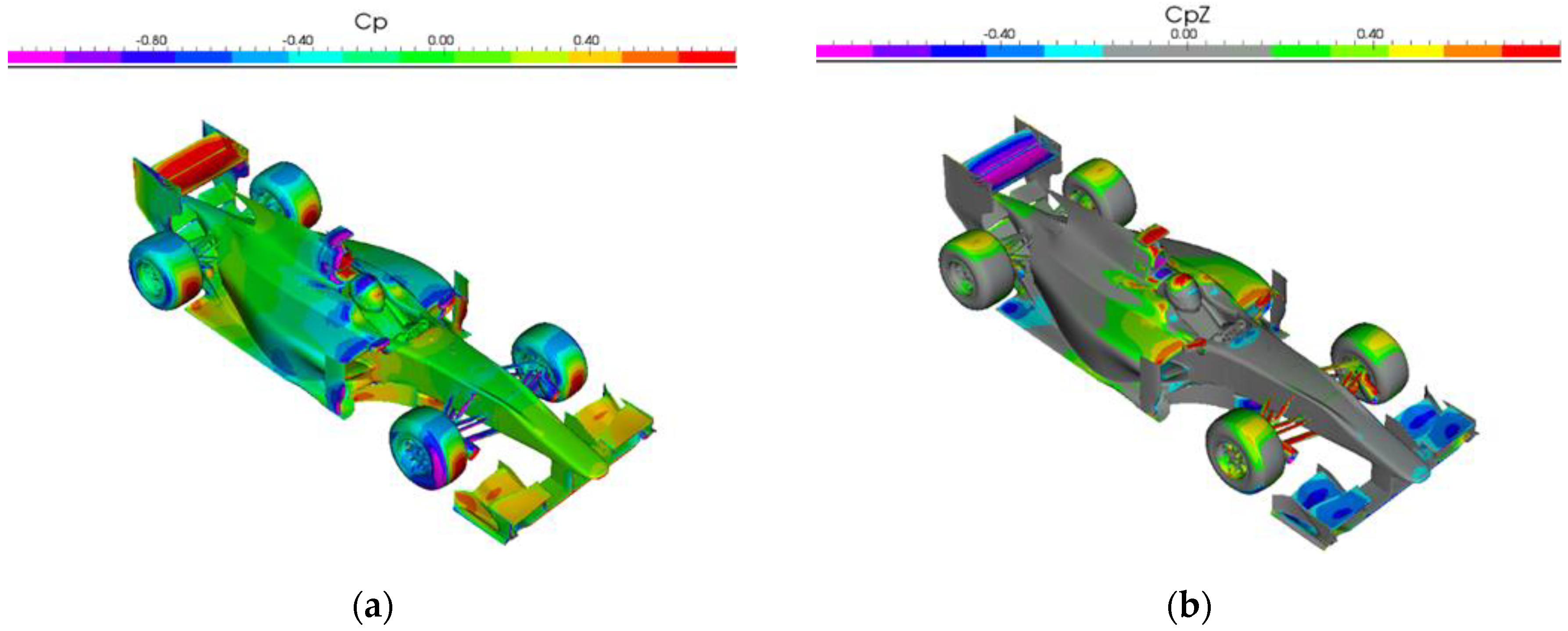
Energies 15 06677 g002
Figure 3. Plots of pressure coefficient Cp and vertical component alone CpZ: (a) pressure distribution over the entire car body; (b) downforce/lift contributions on upper surfaces.
Energies 15 06677 g003
Figure 4. Pressure coefficient Cp in front and rear view: (a) front view showing stagnation pressure areas; (b) rear view showing low pressure areas under rear wing and in underbody Venturi ducts.
Energies 15 06677 g004
Figure 5. Pressure coefficient Cp under the car, showing main downforce contributions through ground effect.
Energies 15 06677 g005
Figure 6. Drag coefficient CDS vs. Front Ride Height FRH and Rear Ride Height RRH. Actual figures are not shown for confidentiality reasons. The percentage variation is computed with reference to maximum drag. Also shown are the ride height ranges: the front one is lower on average and narrower than the rear. Cells with values in red are the areas less likely to tap into: high nose and low tail (high FRH/low RRH, bottom left) and very low nose, high tail (low FRH/high RRH, top right). Background colors highlight the CDS trend: red is the worst (highest) drag zone, while green is the lowest.
Energies 15 06677 g006
Figure 7. Downforce coefficient CZS vs. FRH and RRH. The percentage variation is computed with reference to maximum downforce, corresponding to FRH = 0 mm, RRH = 30 mm. Background colors highlight the CZS trend: in this case green is the best (highest) downforce zone, while red is the lowest.
Energies 15 06677 g007
Figure 8. Aero balance AB vs. FRH and RRH. The variation is computed with reference to the average AB within the map domain, corresponding to FRH = 15 mm, RRH = 40 mm for a pitch angle of 0.46° over a wheelbase of 3.12 m. Background colors in this case highlight the trend of the fore/aft downforce distribution or aero balance with reference to the average value: blue is forward, green is rearward.
Energies 15 06677 g008
Figure 9. Efficiency vs. FRH and RRH, 3D map.
Energies 15 06677 g009
Figure 10. Typical bump stop force vs. deflection curve with “progressive” characteristics.
Energies 15 06677 g010
Figure 11. Evolution of Front vs. Rear Ride Heights for increasing speed, starting from static RH values: (a) speed increases along yellow arrow and the area inside the yellow dotted line is the aero map domain; (b) this is the most significant graph for trackside engineering activities. Vertical red and yellow lines are references for the relevant speed range on a given circuit; yellow markers show where bump stops come into play.
Energies 15 06677 g011
Figure 12. Efficiency vs. Aero Balance and Downforce vs. Drag for the 100–300 kph speed range. Yellow arrows show increasing speed. Dotted lines on the second graph are iso-efficiency levels: (a) Efficiency vs. Aero Balance (b) Downforce vs. Drag. Yellow dots are speed references relevant to a specific circuit.
Energies 15 06677 g012
Figure 13. Aero maps plotted as: (a) Downforce vs. Rear Ride height; (b) Aero Balance vs. Rear Ride Height, for various Front Ride Heights. These graphs highlight non-linear sensitivity to both front and rear ride heights hence to heave and pitch. The evolution in the 0–300 kph range is shown in red. Yellow arrows indicate increasing speed.
Energies 15 06677 g013
Figure 14. Front and rear decay functions starting from static ride heights: (a) RH vs. RH sensitivity; (b) FRH and RRH vs. Speed. Dots and lines as in Figure 11.
Energies 15 06677 g014
Figure 15. Decay effect on ride heights as a function of vehicle speed: (a) efficiency vs. aero balance; (b) downforce vs. drag. Yellow dots are speed references relevant to a specific circuit.
Energies 15 06677 g015
Figure 16. Plots showing vehicle motion with baseline aero maps (#1, blue) and with the application of decay functions (#2, red) along a quasi-static straight-line maneuver with increasing speed. Porpoising is triggered at around 210 kph, with the rear axle coming first and dominating in terms of amplitude. Pitch oscillates with an amplitude above 1 degree and a consistent frequency around 6 Hz.
Energies 15 06677 g016
Figure 17. Comparison of aerodynamic vertical forces with baseline maps (blue) and with decay functions (red). Apart from the oscillations, the average downforce is massively reduced either at the front (top plot) and at the rear (middle plot). Vertical acceleration at the center of gravity (bottom plot) oscillates with an amplitude of +/− 0.6 g.
Energies 15 06677 g017
Figure 18. Comparing amplitudes of front and rear suspension jounce (left) and tire radial deflection (right). The latter is around an order of magnitude larger than the first one: the porpoising phenomenon appears to be dominated by underdamped bouncing on the tires.
Energies 15 06677 g018
Figure 19. Increased front damping (blue plot) results in a slightly reduced amplitude at the rear end (center plot), showing that front and rear axles are strongly coupled through body pitch oscillations (bottom plot). In addition, the modified car can reach a higher speed in the same simulation time: this is due to increased aerodynamic efficiency in terms of drag reduction.
Energies 15 06677 g019
Figure 20. Increased front damping (blue plot) also reduces the amplitude of front suspension jounce (left plots for front and rear axle), the tire deflection is however increased (right plots for front and rear axle). Both amplitudes are reduced at the rear end. Frequencies are basically unaltered.
Energies 15 06677 g020
Figure 21. A stiffer bump stop at the rear axle (blue) basically delays the onset of porpoising from 210 to 220 kph for FRH (top), RRH (center), and pitch oscillation (bottom). Aero efficiency is also affected by a higher rear ride height on average.
Energies 15 06677 g021
Figure 22. Once porpoising oscillations are triggered, average downforce levels are not affected by bump stop stiffness. In this plot front downforce (top), rear downforce (center), and vertical acceleration (bottom) are shown.
Energies 15 06677 g022
Figure 23. Rear suspension jounce amplitude (on the left for front and rear axle) and the delay in terms of speed are the only significant effects of a stiffer bump stop at the rear end (blue plot as always).
Energies 15 06677 g023
Figure 24. Front ride height +10 mm (blue): porpoising is partially mitigated mainly because bouncing is reduced at the front end in terms of amplitude. In this plot FRH (top), RRH (center) and pitch variation (bottom) are shown.
Energies 15 06677 g024
Figure 25. Rear ride height +20 mm (blue): bouncing is significantly reduced at the rear axle and at the front end as well. In this plot FRH (top), RRH (center), and pitch variation (bottom) are shown.
Energies 15 06677 g025
Figure 26. Static ride height variations FRHS +5 mm, RRHS +10 mm (#3, blue): porpoising is remarkably delayed. In this plot FRH (top), RRH (center), and pitch variation (bottom) are shown.
Energies 15 06677 g026
Figure 27. Static ride height variations FRHS +5 mm, RRHS +10 mm (#3, blue): downforce is stable until porpoising is triggered, and higher on average. Efficiency is also improved, and the final simulation speed is higher as well. In this plot front downforce (top), rear downforce (center) and vertical acceleration (bottom) are shown.
Energies 15 06677 g027
Figure 28. Vehicle body motion with static ride height variations FRHS +10 mm, RRHS +20 mm (#4, green) vs. baseline configuration plus decay functions (#2, red) and without (#1, blue). Changes to ride heights and their effects are clearly visible: porpoising is fully removed. In this plot FRH (top), RRH (center), and pitch variation (bottom) are shown.
Energies 15 06677 g028
Figure 29. With the final static ride height variations FRHS +10 mm, RRHS +20 mm (#4, green) the downforce is reduced compared to the original configuration (#1, blue) but porpoising is no longer there. In this plot front downforce (top), rear downforce (center), and vertical acceleration (bottom) are shown.
Energies 15 06677 g029
Figure 30. Porpoising is fully removed with Setup #4 (green), in terms of suspension motion (left plots for front and rear axle) and of tire deflection (right plots for front and rear axle).
Energies 15 06677 g030
Figure 31. Map of the F1 Sakhir circuit in Bahrain, with official corner numbering.
Energies 15 06677 g031
Figure 32. Baseline setup (blue, #1) vs. model with decay functions/porpoising (red, #2). Top plot is the speed profile vs. lap distance, mid and bottom plots are the front and rear ride heights.
Energies 15 06677 g032
Figure 33. Baseline setup (blue, #1) vs. model with decay functions/porpoising (red, #2). Top and mid plot are the front and rear downforce vs. lap distance, bottom plot is the vertical acceleration at the center of gravity.
Energies 15 06677 g033
Figure 34. Setup #3 (purple) vs. #4 (green). Setup #3 is a reasonable tradeoff between the reduction of porpoising (and of driver discomfort as well) and performance in terms of average downforce. Top plot is the speed profile vs. lap distance, mid and bottom plots are the front and rear ride heights.
Energies 15 06677 g034
Figure 35. With Setup #3 porpoising is triggered just at the end of the straight, the downforce level however is higher on average. Top and mid plot are the front and rear downforce vs. lap distance, bottom plot is the vertical acceleration at the center of gravity.
Energies 15 06677 g035
Figure 36. Setup #2 (baseline with porpoising induced by means of the decay functions, red) vs. Setup #3 (FRHS +5 mm, RRHS +10 mm, purple). By raising the ride heights in the correct proportion front to rear porpoising can be reduced without damaging performance too much. Top plot is the speed profile vs. lap distance, mid and bottom plots are the front and rear ride heights.
Energies 15 06677 g036
Table 1. Configurations tested with related lap time. Faster lap time gaps in green, slower in red.
Car Setups and ConfigurationLap TimeGap from (#1) BaselineGap from (#2) Porpoising
(#0) Real-world GP2 car, 4th position in 2013 Qualifying session (Bahrain circuit)1:40.58+0.8%
(#1) Full model, Baseline setup1:39.79=−1.03
(#2) Baseline with porpoising1:40.82+1.03=
(#3) FRHS +5 mm/RRHS +10 mm1:40.32+0.53−0.50
(#4) FRHS +10 mm/RRHS +20 mm1:40.71+0.92−0.11
Publisher’s Note: MDPI stays neutral with regard to jurisdictional claims in published maps and institutional affiliations.

