Bio-Inspired Optimization Algorithms Applied to the GAPID Control of a Buck Converter

Abstract

Although the proportional integral derivative (PID) is a well-known control technique applied to many applications, it has performance limitations compared to nonlinear controllers. GAPID (Gaussian Adaptive PID) is a non-linear adaptive control technique that achieves considerably better performance by using optimization techniques to determine its nine parameters instead of deterministic methods. GAPID represents a multimodal problem, which opens up the possibility of having several distinct near-optimal solutions, which is a complex task to solve. The objective of this article is to examine the behavior of many optimization algorithms in solving this problem. Then, 10 variations of bio-inspired metaheuristic strategies based on Genetic Algorithms (GA), Differential Evolution (DE), and Particle Swarm Optimization (PSO) are selected to optimize the GAPID control of a Buck DC–DC converter. The computational results reveal that, in general, the variants implemented for PSO and DE presented the highest fitness, ranging from 0.9936 to 0.9947 on average, according to statistical analysis provided by Shapiro–Wilks, Kruskall–Wallis and Dunn–Sidak post-hoc tests, considering 95% of confidence level.

1. Introduction

Modern control systems rely on linear mechanisms, as most industries rely on PID (proportional integral derivative) controllers [1]. However, those are constrained by their intrinsic linearity. As a good rule of thumb, higher gain values in a linear PID can lead to faster response times but can cause increased overshoot and the tendency to increase oscillations. In addition, changes in the controlled plant may cause instability in the system [2].

Nonlinear controllers can overcome these limitations but are more complex to design. Adaptive control represents a particular class of nonlinear controllers that share several aspects with linear control, often employed in the industry [3]. Several works deal with adaptive control techniques improving the reference tracking performance while guaranteeing robust behavior under parameter uncertainties [4,5,6,7]. Many of these strategies employ analysis with $H_2$/$H_{\infty }$ norm [8,9] and parameter estimation with Lyapunov theory [10] to ensure convergence and strong capabilities. Such techniques address robust features using adaptive controllers but are not capable of finding the best control parameters. Furthermore, they are not simple and usually require massive calculations.

Adaptive PID is a kind of adaptive control that uses the structure of the PID controller with an adaptive rule for the controller gains [11,12,13]. It is often simpler to implement and presents itself as a good solution for the industry, where PID is already deployed in many facilities. In this case, the design schemes rely on deterministic methods or linear optimizations to achieve reasonable solutions [14,15].

GAPID (Gaussian Adaptive PID) is an adaptive control system that can generate fast and robust control systems with no loss in response quality, such as instability over plant changes or high overshoot levels. Its structure is relatively simple [16]. However, most systems cannot have their parameters determined utilizing deterministic methods. In this sense, bio-inspired optimization algorithms are some of the best mechanisms for dealing with such tasks [17,18,19].

Bio-inspired metaheuristics are inspired by the fundamental relationships among groups of living beings, such as bee colonies or flocks of birds, or even in the genetic mechanisms first stated by Charles Darwin [20,21,22,23]. They have recently gained attention for reasonable solutions for multimodal functions without prior knowledge [24,25]. This behavior is crucial since most real-world problems are challenging because they present multimodality, non-linearity, non-differentiability, and others [26,27].

However, these algorithms present different characteristics (relation between agents, fitness function choices, iterations evolution alternatives, etc.), which can lead to different results and performances for the same problem [25,28].

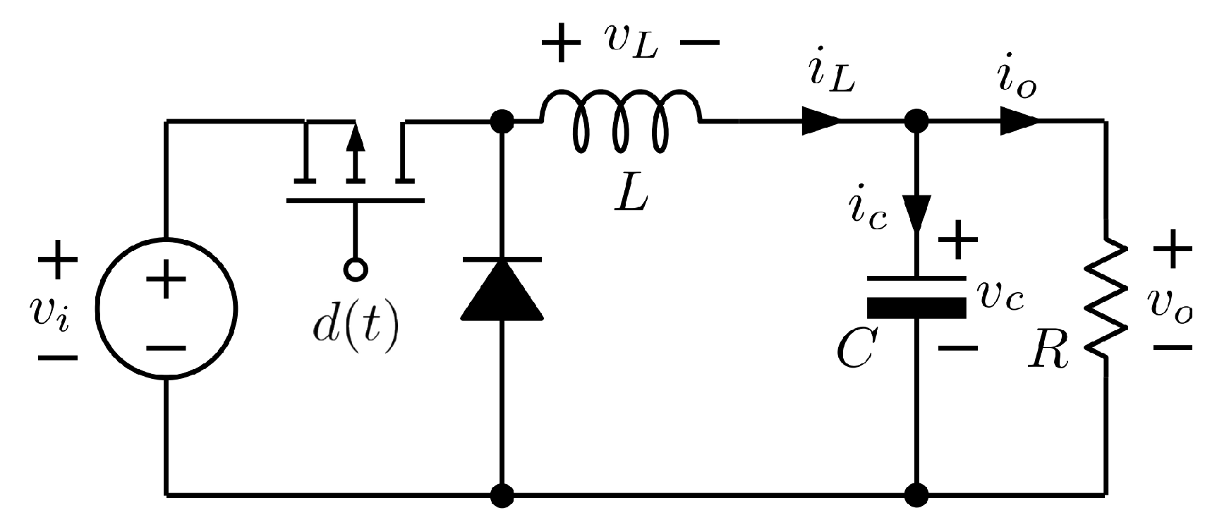
Power converters in the Buck topology are typical step-down converters found in millions of power supplies, mainly for electronic equipment. It operates in a closed loop to stabilize the output voltage supply, demanding a robust controller to guarantee such stabilization. Its mathematical model consists of a second-order plant that can exhibit an underdamped output depending on the operating conditions. A suitable controller is essential to compensate efficiently for this underdamping and other disturbances and provide a good quality power supply. These characteristics justify the purpose of studying optimization methods of adaptive PID for velocity control in this plant.

In this regard, this investigation analyzes and compares the performance of 30 bio-inspired optimization variations, divided equally between versions of Genetic Algorithms (GA), Differential Evolution (DE), Particle Swarm Optimization (PSO) [29], all applied to a GAPID system controlling a Buck converter.

This exhaustive comparison is unprecedented, fills a gap in the literature, and represents this work’s significant contribution. Despite these being the most used algorithms to deal with optimization problems, it must be highlighted that there is still room for an extensive investigation of their application in GAPID [30,31].

In summary, the contributions of this investigation are as follows:

• The insertion of a new metaheuristic method to this analysis (DE);
• The utilization of a varied set of metaheuristics, searching to find better performance when dynamic alterations occur in the plant;
• The application of metaheuristics and their variations in a GAPID controller and implemented in the Buck converter shows that this controller is able to provide optimal performance.

The rest of the paper is organized as follows: Section 2 presents the current state of the art of adaptive control techniques; Section 3 shows the theoretical framework of the GAPID controller; Section 4 discuss the bio-inspired optimization models addressed to tune the GAPID; Section 5 approaches the simulation development with the optimization strategies analysis, performance assessment, and statistical tests; Section 6 presents the results achieved by the optimization methods as well as a critical analysis of such results; Section 7 presents the main conclusions and future works.

2. State of the Art of Adaptive Control Techniques

In [32], the authors proposed an online adaptive fuzzy gain scheduling PID (FGPID) controller for the load frequency control (LFC) of a three-area inter-connected modern power system. The performance was investigated by comparing it with a fixed structure controller. The adaptive terms of the proposed controller were derived from an appropriate Lyapunov function and are not dependent on the controlled system parameters. The results indicated that the proposed FGPID controller performs better than the other fixed structure controllers.

In [33], the authors proposed a controller based on Fuzzy PID using an improved PSO algorithm to perform an adaptive fuzzy PID contour error cross-coupled control method. Compared with the traditional fuzzy PID cross-coupled control method, the fuzzy PID cross-coupled control based on the improved PSO algorithm can reduce the maximum contour error by 53.64%, which has a better control effect.

A comparison of three hybrid approaches (PID-PSO, Fuzzy-PSO, and GA-PSO) for the direct torque control (DTC) and velocity of the dual star induction motor (DSIM) drive was given in [34]. The results showed that the performance of Fuzzy-PSO was better, reducing high torque ripples, improving rise time, and avoiding disturbances affecting the drive performance.

In [35], the authors presented a PID controller based on the BP neural network, a self-tuning PID controller based on an improved BP neural network, with an improved Fletcher–Reeves conjugate gradient method. The presented results showed that the presented method reduced the overshoot of the PID control-based BP neural network, improved the speed of the BP neural network, and reduced the regulating time of PID control.

In [36], a closed-loop motion control system based on a back propagation neural network PID controller by using a Xilinx field programmable gate array (FPGA) solution was proposed. The authors stated that the proposed system could realize the self-tuning of PID control parameters. The results indicated reliable performance, high real-time performance, and strong anti-interference. When compared to traditional MCU-based control methods, the speed convergence of the FPGA-based adaptive control method is much faster than three orders of magnitude, proving its superiority over traditional methods.

In [37], the authors presented another self-adjusting PID controller based on a backpropagation artificial neural network, with GA for offline training, to control the speed of a DC motor. The difference reported was in using the error for network training, the maximum desired values of overshoots, settling times, and stationary errors as input data for the network. As a disadvantage, the authors report that the network’s performance is linked to the operating range of the systems, which implies that the accuracy is not constant and that, therefore, performance may decrease at the limits of system operation.

A time domain performance criterion based on the multi-objective Pareto front solutions was proposed in [38]. The objective function tested was an automatic voltage regulator system (AVR) application using the PSO algorithm. The authors report that the simulation results showed a performance boost compared to traditional objective functions.

The use of PSO and GA methods for tuning the PID controller parameters was presented in [39]. The authors reported that the proposed PSO method could avoid the shortcoming of premature convergence of the GA method, increasing the system performance with more robust stability and efficiency.

In [40], a modified form of the gray wolf optimizer algorithm (GWO) with a novel fitness function has been presented to tune the controller parameters of an FOPID controller to control the terminal voltage of the AVR system, using a modified version of the GWO and a new fitness function. The authors stated robustness in the obtained results compared to other state-of-the-art techniques.

Ouyang and Pano, in [41,42], presented a position domain PID controller for a robotic manipulator that was tuned using three different metaheuristic optimization algorithms. In these works, DE, GA and PSO were used to optimize the gains of the controller alongside three distinct fitness functions for tuning a position domain PID controller (PDC-PID). The authors reported that the PSO and DE algorithms generally performed better than GA, which was always the first to converge.

Studies about the use of bio-inspired optimization algorithms in the design of this controller are being conducted up to the present. This control strategy is challenging to design as it does not have an algebraic solution for the adaptive parameters of the controller.

In this sense, in [43], the authors presented six variations of genetic algorithms for tuning the GAPID and showed good enhancement of GAPID over traditional PID. The authors in [44] did the same six variations but with PSO, which also demonstrated good enhancements of GAPID over PID. These two optimization algorithms also were employed in [17], which were used in a plant based on a step-down DC–DC converter, and compared, demonstrating promising results and a slight advantage for PSO. The latter also presented faster convergence and lower computational cost; however, on the other hand, the agent positions on the last iterations were very concentrated, representing a low search capacity, and possibly converging to a sub-optimal solution instead of the global one.

As for the work in [45], PSO, the Artificial Bee Colony (ABC) algorithm, and the WOA were compared to tuning the Gaussian Adaptive PID controller, considering the Buck converter with a resistive and a nonlinear load as a case study. The authors reported that PSO achieved the best results.

Finally, in [46], the authors analyzed two metaheuristics optimization techniques, GA and PSO, with six variations each and compared them regarding their convergence, quality, and dispersion of solutions. The novelty is that the analysis included plant load variation, thus demanding a modification to the optimization strategy, and, as a result, the controller achieved a more robust behavior. It was reported that the obtained results proved that the GAPID presented fast responses with very low overshoot and good robustness to load changes, with minimal variations, which was impossible to achieve when using the traditional PID.

According to the last cited works, GA and PSO optimization techniques were used to tune the GAPID, and the latter produces better performance when comparing GA with PSO, while the DE was not addressed in these works. In this way, in the present study, a third optimization technique is inserted in order for it to be investigated around its possible variations and finally be compared with the results obtained from GA and PSO.

3. Control Strategy

3.1. Buck Converter

The Buck converter is a DC/DC step-down converter, ubiquitous with DC power supplies for electronic equipment. A pulsed input voltage passes through a low-pass filter to generate the output voltage, which is controlled by a PWM signal that switches the MOSFET [47]. When in steady-state, the input-to-output ratio is given by Equation (1):

$$v_o=v_i·D$$

(1)

where $v_i$ is the input voltage, $v_o$ is the output voltage, and D is the PWM duty cycle that switches the MOSFET. A simple diagram of a Buck converter can be observed in Figure 1.

The state-space equations can describe the dynamics of this converter in Equations (2) and (3).

$$\begin{array}{cc}\hfill \frac{d{i}_L\left(t\right)}{dt}=& \frac{1}{L}\left[-v_o\left(t\right)+V_{i}d\left(t\right)\right]\hfill \end{array}$$

(2)

$$\begin{array}{cc}\hfill \frac{d{v}_o\left(t\right)}{dt}=& \frac{1}{C}\left[i_L\left(t\right)-\frac{1}{R}{v}_o\left(t\right)\right].\hfill \end{array}$$

(3)

In this work, the parameters employed refer to typical power supplies found on some medical equipment. The converter parameters are summarized in

Table 1. Converter parameters.

Parameter	Value
Input voltage	48 V
Output voltage	30 V
Inductor	1.5 mH
Capacitor	10 μF
Load	20 Ω
Switching frequency	30 kHz

.

3.2. GAPID Controller

An adaptive controller is a controller with adjustable parameters and a mechanism for adjusting them [48] and can be thought of as having two feedback loops, one for the process and one for the parameters, as in Figure 2.

The PID is a feedback-based control strategy that uses the error between the plant output and a given set-point to perform the control action based on three gains: proportional ($k_p$), integrative ($k_i$), and derivative ($k_d$) of the error. There is a vast bibliography about PID control systems, and there are many available solving methods for those gains.

The GAPID control, proposed by [43], also explored by Borges et al. [44] and later by Puchta et al. [45], is an Adaptive PID system where each one of the three PID gains ($g_p$, $g_i$, and $g_d$) changes depending on three distinct Gaussian curves and the current error, as shown in Figure 3.

The Gaussian curves are given by Equations (4)–(6), and Figure 4 shows how each parameter affects those curves.

$$\begin{array}{cc}\hfill g_p\left(\sigma \right)& =h_{1p}-(h_{1p}-h_{0p})e^{-q_p{\sigma }^2}\hfill \end{array}$$

(4)

$$\begin{array}{cc}\hfill g_i\left(\sigma \right)& =h_{1i}-(h_{1i}-h_{0i})e^{-q_i{\sigma }^2} \hfill \end{array}$$

(5)

$$\begin{array}{cc}\hfill g_d\left(\sigma \right)& =h_{1d}(1-e^{-q_d{\sigma }^2}) \hfill \end{array}$$

(6)

where:

$\sigma$ is the error signal;

$g_p$, $g_i$ and $g_d$ are adaptive PID gains;

$h_{1p}$, $h_{1i}$ and $h_{1d}$ are the bounds of the Gaussians when error $\to \infty$;

$h_{0p}$ and $h_{0i}$ are the bounds of the Gaussians when error $\to 0$;

$q_p$, $q_i$ and $q_d$ define the degree of concavity of the Gaussians.

The parameter $k_{d0}$ has been set to zero to avoid noise amplification issues when the set-point is reached, and the system operates in steady-state [17], thus leaving the GAPID with eight parameters to be designed: $[h_{0p},h_{1p},h_{0i},$ $h_{1i},h_{1d},q_p,q_i,q_d]$.

One key idea that facilitates its adoption in the industry, where many PID controllers are already deployed, is to link the Gaussian parameters to the PID gains, referred to as linked parameters [17]. It also facilitates the optimization process and increases its reliability. In this technique, the h parameter variables are not free to be assigned any value. The upper and lower bounds of each Gaussian are determined based on their relation to previously designed PID control gains for the same plant.

Those variables are related as can be observed in Equations (7) and (8),

$$\begin{array}{ccc}{h}_{1p}=x{k}_p \hfill & h_{1i}=y{k}_i\hfill & h_{1d}=z{k}_d\hfill \end{array}$$

(7)

$$\begin{array}{ccc}{h}_{0p}=\frac{1}{x}{k}_p \hfill & h_{0i}=\frac{1}{y}{k}_i \hfill & \end{array}$$

(8)

where $k_p$, $k_i$, and $k_d$ are the gains of the previously designed PID, and x, y, and z are new optimization parameters. Meanwhile, $q_p$, $q_i$, and $q_d$ are free parameters, meaning they can take any value in a predetermined range.

The optimization parameters used now are $[x,y,z,q_p,q_i,q_d]$. These will be the vectors of parameters utilized on each optimization strategy and may be referred to by different names: genes, particles, or vectors. These are the characteristics of each solution candidate that create a precise control result.

4. Optimization Strategies

The optimization strategies used in this paper are bio-inspired metaheuristics, which means they are algorithms that utilize natural phenomena as inspiration, such as the evolution by natural selection, in the case of Genetic Algorithms and Differential Evolution, or how groups of animals move through the environment, as in the PSO. The named agent is generically used to define a candidate solution, but each algorithm presents a particular name for them. Below, we describe in detail the GA, DE, and PSO.

4.1. Genetic Algorithm (GA)

A genetic algorithm is an optimization strategy based on the principle of evolution through natural selection [49]. The best-adapted agents (candidate solutions) are more likely to breed and pass their genes (set of parameters) to the next generation, creating a better-optimized population over time [22,50].

The optimization process begins with a randomly generated population of parents (individuals, chromosomes, or agents) that go through selection, crossover, and mutation to create a new generation (offspring) that becomes the parents for the next generation. This process is repeated until a stopping condition is met [49].

4.1.1. Selection

The selection process chooses individuals to participate in the crossover with a bias towards the most well-adapted ones [51,52]. The types of selection addressed in this investigation are as follows:

• Roulette wheel: Each individual is randomly selected from a biased roulette of individuals where the total area that each one occupies is proportional to its fitness value;
• Stochastic Universal Sampling: The selection starts on a random spot on the roulette, and from there, all other individuals are equidistantly chosen on the length of the roulette;
• Binary tournament: Two individuals are picked randomly and compared, and the one with the highest fitness is selected;
• Death tournament: After an individual goes through the tournament process once, it cannot go through it again. Therefore, the loser is suppressed from the population;
• Survival selection: In this case, all individuals participate once in the crossover, generating a population double the original size. After the mutation, a new selection is made from the population of parents and offspring.

4.1.2. Crossover

The crossover process is equivalent to breeding, where a new offspring is created utilizing genes from both parents [25]. The variations of crossover used in this paper are as follows [53]:

• Single-point crossover: The genes of each parent are “cut” in a random place, and the offspring is made from parts of each parent;
• Arithmetic crossover: Each offspring is created by a weighted mean of each parent;
• SBX crossover or simulated binary crossover: Each offspring is created by simulating the characteristics of a binary crossover, such that the parents’ average is equal to the average of the offspring.

4.1.3. Mutation

The mutation process is where new information is added to the current gene pool. The two types of mutation used are as follows [51]:

• Fixed mutation, where each offspring’s gene has a fixed chance of mutating to a new random value;
• Dynamic mutation, where the chance of each gene to mutate is directly proportional to the population’s average fitness.

4.2. Differential Evolution (DE)

Differential Evolution or DE is an evolutionary optimization algorithm that utilizes similar concepts of selection, crossover, and mutation. However, these operators are not the same as in GA and are not used in the same order [54,55].

The optimization process starts by creating a randomly generated population of agents named vectors. Initially, an agent, named target vector ${\mathbf{x}}_i$, is randomly selected among the whole population. The first operation is the mutation, where the target vector is not used [56].

4.2.1. Mutation

The mutation starts generating a weighted difference between randomly selected vectors ${\mathbf{x}}_{r2}$ and ${\mathbf{x}}_{r3}$, which are added to another vector ${\mathbf{x}}_{r1}$, creating the Donor Vector ${\mathbf{v}}_i$, as in Equation (9):

$${\mathbf{v}}_i={\mathbf{x}}_{r1}+F({\mathbf{x}}_{r1}-{\mathbf{x}}_{r2})$$

(9)

where $F\in [0,2]$ is the differential weight, a real constant that determines the step size to be taken to the direction defined by the difference vector.

However, the literature presents some other possibilities for performing the mutation. In this investigation, we also selected the Best mutation (Equation (10)) and Target-to-Best mutation (Equation (11)) [56]:

$$\begin{array}{c}\hfill {\mathbf{v}}_i=\mathbf{xbest}+F({\mathbf{x}}_{r1}-{\mathbf{x}}_{r2})\end{array}$$

(10)

$$\begin{array}{c}\hfill {\mathbf{v}}_i={\mathbf{x}}_{r1}+F(\mathbf{xbest}-{\mathbf{x}}_{r2})\end{array}$$

(11)

with $\mathbf{xbest}$ being the best-positioned candidate solution (higher fitness).

It is also possible to have two weighted vector differences added to the third vector on the mutation, such as in Equation (12):

$${\mathbf{v}}_i={\mathbf{x}}_{r1}+F({\mathbf{x}}_{r2}-{\mathbf{x}}_{r3})+F({\mathbf{x}}_{r4}-{\mathbf{x}}_{r5})$$

(12)

where ${\mathbf{x}}_{r4}$ to ${\mathbf{x}}_{r5}$ are random selected vectors.

4.2.2. Crossover

After mutation, the crossover is applied, and the target vector is used. The procedure creates the trial vector ${\mathbf{u}}_i$. We explored two variants of the crossover operator [31]:

• Binary crossover (bin): For each target vector, a number between 0 and 1 named crossover factor r is randomly generated. If this number is higher than the crossover rate $CR$, previously defined by the user, the current gene (variable value) is picked from the donor vector; otherwise, it is taken from the target vector. At the end of the process, the trial vector will present genes from both donor and target vectors.
• Exponential crossover (exp): The exponential crossover presents similarities with the previous case. The main difference is that the trial vector takes all genes from the target vector until a randomly generated position. After that, the procedure follows the binary one. Therefore, the chance of the new vector being filled with the donor vector drops exponentially.

4.2.3. Selection

The selection on DE is quite simple and works by comparing the fitness of the target vector and trial vector: the one with the highest fitness value is selected, in a greedy procedure.

4.2.4. Nomenclature

Differential Evolution variations receive a notation to ease their description as DE/x/y/z:

• x: type of mutations (rand: Equation (9), best: Equation (10), rand-to-best: Equation (11));
• y: number of weighted differences on the mutation (1 or 2);
• z: type of crossover (bin, exp).

4.3. Particle Swarm Optimization (PSO)

Inspired by the social interactions between groups of animals such as flocks of birds or schools of fish, Particle Swarm Optimization is an optimization method. The particles (candidate solutions or agents) change their current position in the search space based on their own best position achieved so far and the position of the highest fitness considering their neighborhood [57,58]. Equations (13) and (14) show the formulas to obtain the speed and position of each particle at each iteration [59]:

$$\begin{array}{cc}\hfill {\mathbf{v}}_i(t+1)& =\omega {\mathbf{v}}_i\left(t\right)+r_1{c}_1[{\mathbf{pbest}}_i\left(t\right)-{\mathbf{x}}_i\left(t\right)]+r_2{c}_2[\mathbf{gbest}\left(t\right)-{\mathbf{x}}_i\left(t\right)]\hfill \end{array}$$

(13)

$$\begin{array}{cc}\hfill {\mathbf{x}}_i(t+1)& ={\mathbf{x}}_i\left(t\right)+{\mathbf{v}}_i(t+1) \hfill \end{array}$$

(14)

where

i is the index of the current particle;

${\mathbf{x}}_i(t+1)$ is the position of the particle at instant t;

${\mathbf{v}}_i$ is the velocity function of the particle i;

$\omega$ is the inertial factor;

$r_1$ and $r_2$ are random numbers between 0 and 1;

$c_1$ is the personal acceleration factor;

$c_2$ is the social acceleration factor;

$\mathbf{pbest}$ is the best position the particle has seen;

$\mathbf{gbest}$ is the best-known position in the neighborhood.

Each particle can not only memorize its best position ($\mathbf{pbest}$) but can also communicate with other particles and learn their best positions ($\mathbf{gbest}$). The topology of the PSO indicates which particles it can communicate with [60].

The different PSO variations that were explored in this paper are as follows [25]:

• Global topology, where all particles can communicate to all others;
• Ring topology, where the agents can communicate only with two neighbors that are topologically defined;
• Absence initial inertia, where all particles start with a initial velocity ${\mathbf{v}}_{i\left(0\right)}=0$;
• Presence of initial inertia, where all particles start with randomly generated initial velocity ${\mathbf{v}}_{i\left(0\right)}$;
• Decreasing inertial weight $\omega$, where it decreases over time;
• Use of a mutation, very similar to the GA case, where the coordinates of a particle can change randomly;
• Generation of a new population after most of the particles have settled. In this case, all particles are subjected to a random velocity increase.

5. Methodology

In this work, an adaptive controller based on a Gaussian adaptive rule (GAPID) is addressed, which must be properly designed to satisfy the system’s needs with optimal performance. It is a very flexible controller due to the possibility of defining the Gaussian parameters for each adaptive PID gain. However, this also presents a problem: such a definition is not trivial, and no algebraic method exists to determine these parameters. Bio-inspired metaheuristics algorithms are used to accomplish this task. They must deal with a complex challenge because GAPID optimization is a multimodal problem. The main idea is to examine how different algorithms deal with such problems, analyzing their behavior during the optimization iterations and their results regarding the performance, convergence, dispersion, and correlations of the solutions.

Algorithm variations are addressed in approaches to changes in the selection, crossover, and mutation phases—for GA and similarly for DE—although there are other operators to be varied. As for the PSO, the variations are in the initial inertia variation and concerning the topology (ring or global). These algorithm’s variations are presented in Section 4.

All the variations were implemented in MATLAB and SIMULINK, and the performance of the different optimization strategies was analyzed only in the simulation environment.

Graphics about the performance metric parameters (Section 5.2) and statistical methods (Section 5.3) are employed to provide scientific support to present the results (Section 6) and conclusions.

5.1. Optimization Strategies Analysis

In this perspective, three basic algorithms were considered: GA, PSO, and DE metaheuristics [25,31,56,57]. For each optimization strategy, 10 different combinations were developed, totaling 30 distinct variations, which make up a relatively wide universe of analysis and comparison, which are listed and detailed below.

• GA Variations:

• Roulette with a 70% crossover rate, single-point crossover, fixed mutation rate;
• Roulette, single-point crossover, and fixed mutation rate;
• Roulette with survival selection, single-point crossover, fixed mutation rate;
• Tournament, single-point crossover, fixed mutation rate;
• Tournament with survival selection, single-point crossover, fixed mutation rate;
• Death tournament, single-point crossover, fixed mutation rate;
• Stochastic sampling, single-point crossover, fixed mutation rate;
• Tournament, arithmetic crossover, fixed mutation rate;
• Tournament, single-point crossover, dynamic mutation rate;
• Tournament, SBX crossover, fixed mutation rate.

• PSO Variations:

• No initial inertia ${\mathbf{v}}_{i\left(0\right)}=0$, global topology;
• Initial Inertia ${\mathbf{v}}_{i\left(0\right)}$, global topology;
• Decreasing Inertial weight $\omega$, global topology;
• No initial inertia with mutation, global topology;
• No initial inertia with a random velocity increase, global topology;
• No initial inertia, ring topology;
• Initial inertia, ring topology;
• Decreasing inertial weight $\omega$, ring topology;
• No initial inertia with mutation, ring topology;
• No initial inertia with a random velocity increase, ring topology.

• DE Variations:

• Rand/1/Bin;
• Best/1/Bin;
• Rand/2/Bin;
• Target-to-Best/2/Bin;
• Best/2/Bin;
• Rand/1/Exp;
• Best/1/Exp;
• Rand/2/Exp;
• Target-to-Best/2/Exp;
• Best/2/Exp.

It is important to remark that all algorithms must share the same fundamental parameters, such as the size of the population and number of optimization repetitions, leaving only the particular variations parameters mutable, to enable a fair comparison between them. Besides that, knowing that some algorithms follow different concepts of evolution (AG and DE are evolutionary while PSO is swarm movement), special statistical tests such as the Shapiro–Wilks, Kruskall–Wallis, and Dunn–Sidak post-hoc tests were employed to determine the degree of correlation between the solutions of distinct algorithms.

Thus, for each optimization strategy (PSO, GA and DE), 50 agents were considered with a maximum of 100 iterations (stopping criteria) and 30 independent simulations with random uniform initialization.

5.2. Performance Assessment

A performance measurement method addressed to compare different results for the optimizations is used to evaluate the effectiveness of a set of adjusted parameters. The chosen method was the IAE (Integral of Absolute Error), where the modulus of the error between the set-point and the output is integrated. The mathematical expression for the IAE is presented in Equation (15).

$$IAE={\int }_0^{\infty }\left|\sigma \right|dt$$

(15)

The IAE value is then used to create a normalized fitness value between 0 and 1 that determines the quality of each set of parameters [45]. The closer this value is to unity, the better. Equation (16) is used to do so.

$$Fitness=\frac{1}{1+IAE}$$

(16)

5.3. Statistical Tests

It is necessary to apply statistical tests to compare the outputs to fair analyze the results of metaheuristics. Before the analysis, the results must be categorized regarding the parameterization. The Shapiro–Wilk test is a test of normality used in statistics that can determine if a sample of numbers came from a normal distribution [61]. Its null hypothesis is that the samples are normal with unspecified mean and variance. The formula for the Shapiro–Wilk test can be observed in Equation (17):

$$W=\frac{{({\sum }_{i=1}^n{a}_i·x_{\left(i\right)})}^2}{{\sum }_{i=1}^n{(x_i-\overline{x})}^2}$$

(17)

where:

$$\begin{array}{ccc}\hfill (a_1,\cdots ,a_n)=\frac{{\mathbf{m}}^{\mathrm{T}}·{\mathbf{V}}^{-1}}{C}& \hfill & \hfill C=∥{\mathbf{V}}^{-1}·\mathbf{m}∥={({\mathbf{m}}^{\mathrm{T}}·{\mathbf{V}}^{-1}·{\mathbf{V}}^{-1}·\mathbf{m})}^{1/2}\end{array}$$

Vector $\mathbf{m}={(m_1,\cdots ,m_n)}^{\mathrm{T}}$ is created from the expected values of the order statistics of independent and identical distributed random variables sampled from a standard normal distribution, $\mathbf{V}$ is the covariance matrix of those normal order statistics, and $\overline{x}$ is the sample mean.

Based on this normality test, it is usual to observe that part of the results is non-parametric. If this is the case, the following analysis shall apply the Kruskal–Wallis test. If the samples are normally distributed, then ANOVA could be used instead.

Kruskal–Wallis test is a non-parametric method based on ranking for testing whether samples originate from the same distribution [62]. This analysis shows whether the various changes within each strategy changed the outcome of each optimization. The formula for the Kruskal–Wallis test can be observed in Equation (18):

$$H=(N-1)·\frac{{\sum }_{i=1}^g{n}_i{({\overline{r}}_i-\overline{r})}^{{}^2}}{{\sum }_{i=1}^g{\sum }_{j=1}^{n_i}{(r_{ij}-\overline{r})}^2}$$

(18)

where

$n_i$ is the number of observations in group i;

$r_{ij}$ is the rank (among all observations) of observation j from group i;

N is the total number of observations across all groups;

${\overline{r}}_i=\frac{{\sum }_{j=1}^{n_i}{r}_{ij}}{n_i}$;

and $\overline{r}=\frac{1}{2}·(N+1)$ is the average rank of all observations on group i.

The third statistical test addressed is the Dunn–Sidak correction as a Post-Hoc analysis. This family-wise error test corrects for multiple comparisons through Equation (19), comparing each pair of fitness results samples.

$${\alpha }^{*}=1-{(1-\alpha )}^{\frac{1}{k}}$$

(19)

where k is a different null hypothesis of $\alpha$ significance level. Each null hypothesis that has a p-value under ${\alpha }^{*}$ is rejected.

The null hypothesis of this test is as follows: for each paired comparison, the probability of a randomly selected value from one group is more extensive than a randomly selected value from the second group equals one-half, which can be understood as a median comparison test. When rejecting the null hypothesis, this test stipulates a significant difference between those two results.

To determine the validity of the results, Shapiro–Wilks p-test values are calculated for these cases. For that, 30 simulations of each variation were considered.

6. Experiments and Results

This section reports the results from the 30 addressed algorithm variations applied to the GAPID control of a buck converter. The experiments were performed using MATLAB and Simulink.

The Simulink model used in the simulations is depicted in Figure 5, and the structure of the GAPID is presented in Figure 6. The parameters of the Gaussian functions are continuously updated during the optimization process in the block “Gaussian”. The results are captured in the scopes as data vectors, to be processed and to have their IAE value calculated.

Table 2. Fitness values for different variations of GA, DE, and PSO.

Optimizer	Highest Fit.	Mean Fit.	Standard Deviation
GA 1	0.9934	0.9904	0.0021
GA 2	0.9927	0.9909	0.0017
GA 3	0.9927	0.9935	0.0029
GA 4	0.9935	0.9917	0.0024
GA 5	0.9930	0.9880	0.0031
GA 6	0.9933	0.9917	0.0015
GA 7	0.9933	0.9904	0.0020
GA 8	0.9915	0.9896	0.0015
GA 9	0.9929	0.9906	0.0022
GA 10	0.9940	0.9915	0.0012
DE 1	0.9943	0.9920	0.0009
DE 2	0.9965	0.9947	0.0009
DE 3	0.9947	0.9935	0.0007
DE 4	0.9962	0.9935	0.0016
DE 5	0.9962	0.9934	0.0012
DE 6	0.9933	0.9915	0.0010
DE 7	0.9956	0.9939	0.0007
DE 8	0.9934	0.9921	0.0010
DE 9	0.9947	0.9919	0.0012
DE 10	0.9954	0.9926	0.0013
PSO 1	0.9946	0.9935	0.0021
PSO 2	0.9951	0.9934	0.0012
PSO 3	0.9951	0.9932	0.0012
PSO 4	0.9946	0.9936	0.0006
PSO 5	0.9947	0.9930	0.0013
PSO 6	0.9937	0.9925	0.0012
PSO 7	0.9943	0.9921	0.0013
PSO 8	0.9947	0.9922	0.0013
PSO 9	0.9941	0.9926	0.0007
PSO 10	0.9940	0.9918	0.0011

Note: the best fitness value for each optimizer is highlighted.

shows the best values of fitness found for each optimization strategy alongside their mean and standard deviation values considering the 30 executions. The numbers in bold represent the highest fitness, highest mean fitness, and slightest standard deviation presented by each strategy (GA, DE, and PSO).

Based on these results, Figure 7 presents a boxplot considering each algorithm’s fitness of the 30 runs. Note that GA variations are in green, PSO variations in blue, and DE variations in red.

During the execution of the algorithms, it was observed that the DE tends to use a greater number of iterations until convergence due to the crossover rate $CR$ of 0.3, since it is possible to generate a greater number of iterations with the same computational power than other strategies.

Table 2 and boxplot in Figure 7 reveal that GA showed variations with higher dispersion, with some of them being poor optimizers. One can observe that GA3 and GA5, which present the survival selection, single-point crossover, and fixed mutation rate, were the worst candidates. The PSO variations presented a more uniform behavior, especially the first four variations. In addition, it can be noted that the peaks in the boxplot were achieved by the DE variations, which also presented the highest mean fitness.

In the first view, one can observe that GA 10, DE 2, and PSO 2 achieved the best overall performance for each algorithm (highest fitness) regarding the 30 executions, highlighting DE 2. Regarding average fitness, GA 6, DE 2, and PSO 4 stood out considering the same algorithm.

It is important to observe that the GAPID parameters are linked to the PID gains, which means that GAPID represents a real improvement over the PID as they share the same design requirements, as can be seen in the IAE values shown in

Table 3. IAE values of PID and GAPID.

Control	PID	GAPID (GA 10)	GAPID (PSO 2)	GAPID (DE 2)
IAE	0.0125	0.0060	0.0049	0.0035

, where the lower the value, the better.

Figure 8 shows the best, worst, and average fitness for each generation along the evolutionary process for the best run of DE 2. One can see from the blue curve that the algorithm presents a fast convergence, reaching, in this case, a result close to the maximum fitness achievable ($fit=1$).

As a complex multimodal problem, one of the difficulties in finding the optimum point is that different input values are likely to result in similar fitness values. The best parameters found in each strategy are recorded in

Table 4. Best set of parameters considering the highest fitness found by each algorithm.

	x	y	z	${\mathit{q}}_{\mathit{p}}$	${\mathit{q}}_{\mathit{i}}$	${\mathit{q}}_{\mathit{d}}$	Fitness
GA 10	15.988	0.631	17.356	0.005	0.003	0.0040	0.9940
DE 2	17.506	0.373	7.843	0.044	0.001	0.0802	0.9965
PSO 2	18.295	0.394	10.260	0.005	0.003	0.0090	0.9951

to present how different simulations found different local optima points.

Considering these findings, we present in Figure 9 the response to the input step of 30 V considering the best set of parameters found by the GA 10, DE 2, PSO 2 for GAPID and the original PID control. It’s important to note that to make the waveforms easier to see, the PWM block has been contoured to hide the switching effects on the waveforms. The figure shows how the adaptive nature of the GAPID can lead to faster transient responses without destabilization. In Figure 10 and Figure 11, the outputs of the PID and GAPID are presented, but in this case, the PWM is considered, switching at 30 kHz.

By analyzing the waveforms, only GAPID optimized by DE 2 presented an overshoot, which was 1.04%, which means the DE resulted in slightly higher gains for GAPID, with a shorter rise time when compared to PSO and GA. In the case of the Buck converter, where the main objective is to generate a regulated output voltage, it does not pose a problem, but depending on the target application, this can be undesirable behavior. The responses of GAPID optimized by PSO and GA are fast and smooth, without overshoot, with a slight advantage over PSO, which can be seen as the best candidate solution to GAPID if overshoot is not allowable. GAPID optimized by PSO and GA perform quite similarly, but GAPID-DE is considerably distinct. That evidences the multimodal characteristic of the GAPID problem where all these solutions have a similar highest level of fitness.

6.1. Statistical Tests Application

To fairly compare the results from the different variations of the GA, DE, and PSO strategies, we applied Shapiro–Wilks, Kruskall–Wallis, and Dunn–Sidak tests, all with a significance level of $\alpha =0.05$.

As a way to determine the validity of the results, the p-values of the Shapiro–Wilks test are presented, considering the 30 simulations of each variation in

Table 5. Shapiro–Wilks test results for GA, PSO, and DE.

GA	p-Value	N-h.	PSO	p-Value	N-h.	DE	p-Value	N-h.
GA 1 *	0.3124	0	DE 1	0.0000	1	PSO 1 *	0.5330	0
GA 2	0.0341	1	DE 2	0.0001	1	PSO 2	0.0357	1
GA 3	0.0100	1	DE 3 *	0.0754	0	PSO 3 *	0.1113	0
GA 4	0.0003	1	DE 4 *	0.4394	0	PSO 4 *	0.6388	0
GA 5 *	0.1056	0	DE 5	0.0008	1	PSO 5 *	0.0838	0
GA 6	0.0022	1	DE 6	0.0070	1	PSO 6 *	0.7055	0
GA 7 *	0.2515	0	DE 7 *	0.4101	0	PSO 7 *	0.3818	0
GA 8	0.0001	1	DE 8 *	0.4819	0	PSO 8 *	0.0729	0
GA 9 *	0.0577	0	DE 9 *	0.1726	0	PSO 9 *	0.4756	0
GA 10*	0.9962	0	DE 10 *	0.3508	0	PSO 10 *	0.3828	0

Note 1: “N-h.” is the “null-hypothesis” of the statistical test. Note 2: The * indicates which strategies have null-hypothesis “0”.

, in order to evaluate the normality of the outputs (the values in bold with an asterisk are those that rejected the null hypothesis).

Table 5 reveals that after applying the Shapiro–Wilks test, most of the results were non-parametric (the errors are not from a normal distribution): GA 2, GA 3, GA 4, GA 6, GA 8, PSO 2, DE 1, DE 2, DE 4, and DE 6. In this sense, we considered non-parametric tests for the obtained results.

Then, the Kruskal–Wallis test was applied to each of the three main optimization strategies’ results. The p-values found were $9.566\times {10}^{-11}$ for GA, $3.0844\times {10}^{-28}$ for DE and $1.379\times {10}^{-11}$ for PSO. Since all three p-values were lower than the standard $\alpha =0.05$ limit, it can be considered that all variations led to a differential factor for the GAPID control performance.

Finally, the Dunn–Sidak correction post-hoc analysis was applied.

Table 6. Dunn–Sidak test results for GA 10, DE 2, and PSO 2.

GA 10	GA 1	GA 2	GA 3	GA 4	GA 5	GA 6	GA 7	GA 8	GA 9
DE 2	DE 1	DE 3	DE 4	DE 5	DE 6	DE 7	DE 8	DE 9	DE 10
PSO 2	PSO 1	PSO 3	PSO 4	PSO 5	PSO 6	PSO 7	PSO 8	PSO 9	PSO 10

Note: In this table, the highlighted cells indicate when there is a statistically significant difference between the two variations, considering light green for GA, light red for DE, and light blue for PSO.

presents the results comparing the variations that achieved the highest fitness (GA 10, DE 2, and PSO 2) with the other nine variations of the same algorithm on each row. When there is a significant statistical difference between the two variations, the corresponding cell is highlighted with light green for GA, light red for DE, and light blue for PSO.

As observed, the application of the test in the best genetic algorithm variation (GA 10—tournament, SBX crossover, 100% crossover rate, fixed mutation rate) did not reject the null hypothesis on the cases for GA 1 (roulette with a 70% crossover rate, single-point crossover, fixed mutation rate), GA 2 (roulette, single-point crossover, fixed mutation rate), GA 4 (tournament, single-point crossover, fixed mutation rate), GA 6 (death tournament, single-point crossover, fixed mutation rate), GA 7 (stochastic sampling, single-point crossover, fixed mutation rate), and GA 9 (tournament, single-point crossover, dynamic mutation rate), meaning that they are statistically equivalent.

For the Particle Swarm Optimization, the variations PSO 1 (no initial inertia, global topology), PSO 3 (decreasing inertia, global topology), PSO 4 (no initial inertia with mutation, global topology), PSO 5 (no initial inertia with a bomb, global topology), and PSO 6 (no initial inertia, ring topology) variations were considered to be statistically similar to the best candidate PSO 2 (initial inertia, global topology).

For DE with the best overall response, DE 2 (Best/1/Bin), the null hypothesis was accepted for DE 3 (Rand/2/Bin), DE 5 (Best/2/Bin), and DE 7 (Best/1/Exp).

Beyond the pairwise comparison for each GA variation with GA 10, each DE variation with DE 2, and each PSO variation with PSO 2 presented in Table 6, we compared the DE 2 to the variations of other strategies. From these comparisons, the variations PSO 1, PSO2, PSO 3, and PSO 4 presented statistical similarity, while no GA variation was able to match that fitness value.

In summary, the overall best strategies variations were PSO 1, PSO 2, PSO 3, PSO 4, DE 3, DE 4, DE 5, and DE 7, while DE 2 presented the highest fitness. According to the Dunn–Sidak correction, these strategies have no statistical difference.

6.2. General Analysis: Algorithms Application

Analyzing the boxplots, Shapiro–Wilks, Kruskal–Wallis, and Dunn–Sidak test results, and the response to a step signal, it is possible to come up with some general observations:

For GAs:

• Roulette-based strategies (GA 1 and 2) have an overall worse performance when compared to the tournament strategy (GA 4);
• The stochastic sampling selection (GA 7) had lower fitness values when compared to the roulette (GA 2) and tournament (GA 4) strategies;
• The survival selection (GA 3 and 5) was not beneficial for this optimization problem;
• The death tournament (GA 6) resulted in a lower standard variation when compared to the regular tournament (GA 4);
• The arithmetic crossover (GA 8) was not able to find high-quality parameters;
• The dynamic mutation (GA 9) had an increased spread but with no real performance gain;
• The SBX crossover (GA 10) obtained the best results for the tested GA variations. However, analyzing the Dunn–Sidak results, this strategy is statistically similar to the strategies GA 1, GA 4, GA 6, and GA 7.

For PSO:

• Global topology (PSO 1 through 5) performed better than their ring topology counterparts (PSO 6 through 10);
• Both decreasing inertia strategies (PSO 3 and PSO 7) offered the second and third lowest PSO errors, respectively;
• The mutation variation (PSO 4 and 9) lowered the results spread and its optimizations were, on average, better than the other variations;
• The random velocity increase (PSO 5 and 10) did not appear to have improved the performance of optimization;
• The initial inertia variation with global topology (PSO 2) offered the highest fitness values for PSO strategies, but analyzing the Dunn–Sidak correction, this variation can be considered tied in efficiency to PSO 5 and PSO 7.

For DEs:

• In general, Differential Evolution strategies achieved lower error values than both GAs and PSO strategies;
• The binary crossover (DE 1 to 5) generally achieved better agents when compared to the exponential crossover (DE 6 to 10);
• Rand/1 type strategies (DE 1 and 6) showed lower performance compared to other DEs;
• Best/1 variations (DE 2 and 7) was the best mutation variation found on DE high-quality results;
• Rand/2, Target-to-best, and Best/2 variations produced, in general, low fitness individuals compared to the best strategies,

In summary, the results showed that some variations of the algorithms could reach similar performances, despite the real response in the GAPID be not the same (see Figure 9). However, analyzing the best performance achievable (Table 2), the average performance (Figure 7), and the smaller dispersion (Figure 7), there is a strong indication that DE 2 is the most reasonable choice, even if it presents statistical similarity with other proposals.

7. Conclusions and Recommendation

In this work, we analyzed several variants of metaheuristic techniques to find the parameters of the GAPID control of a Buck converter. As far as we know, there is no broad comparative study related to metaheuristics applied to optimize the GAPID controller parameters.

We discuss the most relevant works on Buck converters, linear and adaptive control, and metaheuristic optimization, especially GA, DE, and PSO. A GAPID-controlled Buck converter was implemented using the MATLAB/Simulink platform, and experiments were carried out with 10 different variants of each of the GA, DE, and PSO algorithms.

The results obtained from each variant were compared using the Shapiro–Wilk normality test and then the Kruskall–Wallis and Dunn–Sidak statistical tests for non-parametric data. We found that the fitness values from some DE and PSO variants present a better performance than GA strategy, especially when PSO considers global topology and DE considers binary crossover. However, the highest fitness was achieved by the DE 2 (Best/1/Bin).

In future work, further analysis can be done by applying the DE and PSO variants to tune different PID controllers and also studying the behavior of these metaheuristics using an automatic hyperparameter tuning approach on-the-fly. We highlight that the use of multi-objective approaches in such a problem is still an open question.

References

1. Ogata, K. Modern Control Engineering, 4th ed.; Prentice Hall PTR: Hoboken, NJ, USA, 2001. [Google Scholar]
2. Filho, A.C.B.B. Principles of Instability and Stability in Digital PID Control Strategies and Analysis for a Continuous Alcoholic Fermentation Tank Process Start-up. Preprints 2018. [Google Scholar] [CrossRef]
3. Narendra, K. Applications of Adaptive Control; Elsevier Science: Amsterdam, The Netherlands, 2012. [Google Scholar]
4. Krstić, M.; Kokotović, P.V.; Kanellakopoulos, I. Transient-performance improvement with a new class of adaptive controllers. Syst. Control Lett. 1993, 21, 451–461. [Google Scholar] [CrossRef]
5. Hsia, T. Adaptive control of robot manipulators—A review. In Proceedings of the 1986 IEEE International Conference on Robotics and Automation, San Francisco, CA, USA, 7–10 April 1986; Volume 3, pp. 183–189. [Google Scholar] [CrossRef]
6. Zhang, Y.; Ioannou, P.; Chien, C.C. Parameter convergence of a new class of adaptive controllers. IEEE Trans. Autom. Control 1996, 41, 1489–1493. [Google Scholar] [CrossRef]
7. Wen, J.T.; Bayard, D.S. Simple robust control laws for robot manipulators: Part 1: Non-adaptive case. In Proceedings of the Workshop on Space Telerobotics, Pasadena, CA, USA, 20–22 January 1987; Volume 3. [Google Scholar]
8. Kyu Park, S.; Kyun Ahn, H. A Design of the H2/H Robust Controller for Adaptive Control Systems-Polynomial Approach. In Proceedings of the IFAC Symposium on System Identification (SYSID’97), Kitakyushu, Fukuoka, Japan, 8–11 July 1997; Volume 30, pp. 1423–1426. [Google Scholar] [CrossRef]
9. Sedhom, B.E.; Hatata, A.Y.; El-Saadawi, M.M.; Abd-Raboh, E.H.E. Robust adaptive H-infinity based controller for islanded microgrid supplying non-linear and unbalanced loads. IET Smart Grid 2019, 2, 420–435. [Google Scholar] [CrossRef]
10. Na, J.; Huang, Y.; Liu, T.; Zhu, Q. Reinforced adaptive parameter estimation with prescribed transient convergence performance. Syst. Control Lett. 2021, 149, 104880. [Google Scholar] [CrossRef]
11. Fahmy, R.A.; Badr, R.I.; Rahman, F.A. Adaptive PID Controller Using RLS for SISO Stable and Unstable Systems. Adv. Power Electron. 2014, 2014, 507142. [Google Scholar] [CrossRef]
12. Anderson, K.; Blankenship, G.; Lebow, L. A rule-based adaptive PID controller. In Proceedings of the 27th IEEE Conference on Decision and Control, Austin, TX, USA, 7–9 December 1988; Volume 1, pp. 564–569. [Google Scholar] [CrossRef]
13. Radke, F.; Isermann, R. A parameter-adaptive PID-controller with stepwise parameter optimization. Automatica 1987, 23, 449–457. [Google Scholar] [CrossRef]
14. Jung, J.W.; Leu, V.Q.; Do, T.D.; Kim, E.K.; Choi, H.H. Adaptive PID Speed Control Design for Permanent Magnet Synchronous Motor Drives. IEEE Trans. Power Electron. 2015, 30, 900–908. [Google Scholar] [CrossRef]
15. Kong, Y.; Jiang, Y.; Zhou, J.; Wu, H. A time controlling neural network for time-varying QP solving with application to kinematics of mobile manipulators. Int. J. Intell. Syst. 2021, 36, 403–420. [Google Scholar] [CrossRef]
16. Puchta, E.D.; Lucas, R.; Ferreira, F.R.; Siqueira, H.V.; Kaster, M.S. Gaussian adaptive PID control optimized via genetic algorithm applied to a step-down DC-DC converter. In Proceedings of the 2016 12th IEEE International Conference on Industry Applications (INDUSCON), Curitiba, Brazil, 20–23 November 2016; pp. 1–6. [Google Scholar]
17. Puchta, E.D.; Siqueira, H.V.; Kaster, M.d.S. Optimization Tools Based on Metaheuristics for Performance Enhancement in a Gaussian Adaptive PID Controller. IEEE Trans. Cybern. 2020, 50, 1185–1194. [Google Scholar] [CrossRef]
18. Khanesar, M.A.; Lu, J.; Smith, T.; Branson, D. Electrical load prediction using interval type-2 Atanassov intuitionist fuzzy system: Gravitational search algorithm tuning approach. Energies 2021, 14, 3591. [Google Scholar] [CrossRef]
19. Elsisi, M. Optimal design of nonlinear model predictive controller based on new modified multitracker optimization algorithm. Int. J. Intell. Syst. 2020, 35, 1857–1878. [Google Scholar] [CrossRef]
20. Santos, P.; Macedo, M.; Figueiredo, E.; Santana, C.J.; Soares, F.; Siqueira, H.; Maciel, A.; Gokhale, A.; Bastos-Filho, C.J. Application of PSO-based clustering algorithms on educational databases. In Proceedings of the 2017 IEEE Latin American Conference on Computational Intelligence (LA-CCI), Arequipa, Peru, 8–10 November 2017; pp. 1–6. [Google Scholar]
21. Belotti, J.T.; Castanho, D.S.; Araujo, L.N.; da Silva, L.V.; Alves, T.A.; Tadano, Y.S.; Stevan, S.L., Jr.; Correa, F.C.; Siqueira, H.V. Air pollution epidemiology: A simplified Generalized Linear Model approach optimized by bio-inspired metaheuristics. Environ. Res. 2020, 191, 110106. [Google Scholar] [CrossRef] [PubMed]
22. Siqueira, H.; Macedo, M.; Tadano, Y.d.S.; Alves, T.A.; Stevan, S.L.; Oliveira, D.S.; Marinho, M.H.; Neto, P.S.; de Oliveira, J.F.; Luna, I.; et al. Selection of temporal lags for predicting riverflow series from hydroelectric plants using variable selection methods. Energies 2020, 13, 4236. [Google Scholar] [CrossRef]
23. Junior, J.J.A.M.; Freitas, M.L.; Siqueira, H.V.; Lazzaretti, A.E.; Pichorim, S.F.; Stevan, S.L., Jr. Feature selection and dimensionality reduction: An extensive comparison in hand gesture classification by sEMG in eight channels armband approach. Biomed. Signal Process. Control 2020, 59, 101920. [Google Scholar] [CrossRef]
24. Eberhart, R.C.; Shi, Y.; Kennedy, J. Swarm Intelligence; Elsevier: Amsterdam, The Netherlands, 2001. [Google Scholar]
25. De Castro, L.N. Fundamentals of Natural Computing: Basic Concepts, Algorithms, and Applications; CRC Press: Boca Raton, FL, USA, 2006. [Google Scholar]
26. de Souza Tadano, Y.; Siqueira, H.V.; Alves, T.A. Unorganized machines to predict hospital admissions for respiratory diseases. In Proceedings of the 2016 IEEE Latin American Conference on Computational Intelligence (LA-CCI), Cartagena, CA, USA, 2–4 November 2016; pp. 1–6. [Google Scholar]
27. Ribeiro, V.H.A.; Reynoso-Meza, G.; Siqueira, H.V. Multi-objective ensembles of echo state networks and extreme learning machines for streamflow series forecasting. Eng. Appl. Artif. Intell. 2020, 95, 103910. [Google Scholar] [CrossRef]
28. Siqueira, H.; Santana, C.; Macedo, M.; Figueiredo, E.; Gokhale, A.; Bastos-Filho, C. Simplified binary cat swarm optimization. Integr. Comput.-Aided Eng. 2021, 28, 35–50. [Google Scholar] [CrossRef]
29. Niccolai, A.; Bettini, L.; Zich, R. Optimization of electric vehicles charging station deployment by means of evolutionary algorithms. Int. J. Intell. Syst. 2021. [Google Scholar] [CrossRef]
30. Eiben, A.E.; Smith, J.E. (Eds.) Introduction to Evolutionary Computing; Springer: Berlin, Germany, 2016. [Google Scholar]
31. Price, K.; Storn, R.M.; Lampinen, J.A. Differential Evolution: A Practical Approach to Global Optimization; Springer Science & Business Media: Berlin, Germany, 2006. [Google Scholar]
32. Razmi, P.; Rahimi, T.; Sabahi, K.; Gheisarnejad, M.; Khooban, M.H. Adaptive fuzzy gain scheduling PID controller for frequency regulation in modern power system. IET Renew. Power Gener. 2022. [Google Scholar] [CrossRef]
33. Ji, W.; Cui, X.; Xu, B.; Ding, S.; Ding, Y.; Peng, J. Cross-coupled control for contour tracking error of free-form curve based on fuzzy PID optimized by improved PSO algorithm. Meas. Control 2009, 25, 323–333. [Google Scholar] [CrossRef]
34. Boukhalfa, G.; Belkacem, S.; Chikhi, A.; Benaggoune, S. Genetic algorithm and particle swarm optimization tuned fuzzy PID controller on direct torque control of dual star induction motor. J. Cent. South Univ. 2019, 26, 1886–1896. [Google Scholar] [CrossRef]
35. Jiangming, K.; Jinhao, L. Self-Tuning PID controller based on improved BP neural network. In Proceedings of the 2009 Second International Conference on Intelligent Computation Technology and Automation, Changsha, China, 10–11 October 2009; Volume 1, pp. 95–98. [Google Scholar]
36. Wang, J.; Li, M.; Jiang, W.; Huang, Y.; Lin, R. A Design of FPGA-Based Neural Network PID Controller for Motion Control System. Sensors 2022, 22, 889. [Google Scholar] [CrossRef] [PubMed]
37. Rodríguez-Abreo, O.; Rodríguez-Reséndiz, J.; Fuentes-Silva, C.; Hernández-Alvarado, R.; Falcón, M.D.C.P.T. Self-tuning neural network PID with dynamic response control. IEEE Access 2021, 9, 65206–65215. [Google Scholar] [CrossRef]
38. Sahib, M.A.; Ahmed, B.S. A new multiobjective performance criterion used in PID tuning optimization algorithms. J. Adv. Res. 2016, 7, 125–134. [Google Scholar] [CrossRef] [PubMed]
39. Ou, C.; Lin, W. Comparison between PSO and GA for parameters optimization of PID controller. In Proceedings of the 2006 International Conference on Mechatronics and Automation, Luoyang, China, 25–28 June 2006; pp. 2471–2475. [Google Scholar]
40. Nasir, M.; Khadraoui, S. Fractional-order PID Controller Design Using PSO and GA. In Proceedings of the 2021 14th International Conference on Developments in eSystems Engineering (DeSE), Sharjah, United Arab Emirates, 7–10 December 2021; pp. 192–197. [Google Scholar]
41. Pano, V.; Ouyang, P.R. Comparative study of ga, pso, and de for tuning position domain pid controller. In Proceedings of the 2014 IEEE International Conference on Robotics and Biomimetics (ROBIO 2014), Bali, Indonesia, 5–10 December 2014; pp. 1254–1259. [Google Scholar]
42. Ouyang, P.; Pano, V. Comparative study of DE, PSO and GA for position domain PID controller tuning. Algorithms 2015, 8, 697–711. [Google Scholar] [CrossRef]
43. Kaster, M.; Borges, F.; Filho, M.; Siqueira, H.; Correa, F. Comparison of Several Genetic Algorithm Strategies on a nonlinear GAPID Controller Optimization Applied to a Buck Converter. In Proceedings of the Congresso Brasileiro de Automatica (CBA), João Pessoa, Brazil, 9–12 September 2018. [Google Scholar]
44. Borges, F.; Monteiro, L.; Martins, S.; Correia, F.; Siqueira, H.; Kaster, M. Performance Comparison of Particle Swarm optimization Strategies to Adjust a Nonlinear GAPID Controller. In Proceedings of the IEEE/IAS International Conference on Industry Applications, Portland, OR, USA, 23–27 September 2018; pp. 685–691. [Google Scholar]
45. Puchta, E.D.P.; Bassetto, P.; Biuk, L.H.; Itaborahy Filho, M.A.; Converti, A.; Kaster, M.D.S.; Siqueira, H.V. Swarm-Inspired Algorithms to Optimize a Nonlinear Gaussian Adaptive PID Controller. Energies 2021, 14, 3385. [Google Scholar] [CrossRef]
46. Borges, F.G.; Guerreiro, M.; Sampaio Monteiro, P.E.; Janzen, F.C.; Corrêa, F.C.; Stevan, S.L.; Siqueira, H.V.; Kaster, M.D.S. Metaheuristics-Based Optimization of a Robust GAPID Adaptive Control Applied to a DC Motor-Driven Rotating Beam with Variable Load. Sensors 2022, 22, 6094. [Google Scholar] [CrossRef]
47. Wu, K.C. (Ed.) Chapter 1—Isolated Step-Down (Buck) Converter. In Switch-Mode Power Converters; Academic Press: Cambridge, MA, USA, 2006; pp. 1–48. [Google Scholar]
48. Astrom, K.J.; Wittenmark, D.B. Adaptive Control, 2nd ed.; Dover Publications, Inc.: New York, NY, USA, 2008. [Google Scholar]
49. Holland, J. Adaptation in Natural and Artificial Systems: An Introductory Analysis with Applications to Biology, Control, and Artificial Intelligence; University of Michigan Press: Ann Arbor, MI, USA, 1975. [Google Scholar]
50. Guerreiro, M.T.; Guerreiro, E.M.A.; Barchi, T.M.; Biluca, J.; Alves, T.A.; de Souza Tadano, Y.; Trojan, F.; Siqueira, H.V. Anomaly Detection in Automotive Industry Using Clustering Methods—A Case Study. Appl. Sci. 2021, 11, 9868. [Google Scholar] [CrossRef]
51. Bäck, T.; Fogel, D.B.; Michalewicz, Z. Evolutionary Computation 1: Basic Algorithms and Operators; CRC Press: Boca Raton, FL, USA, 2018. [Google Scholar]
52. Pencheva, T.; Atanassov, K.; Shannon, A. Modelling of a stochastic universal sampling selection operator in genetic algorithms using generalized nets. In Proceedings of the Tenth International Workshop on Generalized Nets, Sofia, Bulgaria, 5 December 2009; pp. 1–7. [Google Scholar]
53. Deb, K.; Sindhya, K.; Okabe, T. Self-adaptive simulated binary crossover for real-parameter optimization. In Proceedings of the 9th Annual Conference on Genetic and Evolutionary Computation, London, UK, 7–11 July 2007; pp. 1187–1194. [Google Scholar]
54. Storn, R.; Price, K. Differential Evolution—A Simple and Efficient Heuristic for global Optimization over Continuous Spaces. J. Glob. Optim. 1997, 11, 341–359. [Google Scholar] [CrossRef]
55. Abdi, H.; Moradi, M.; Lumbreras, S. Metaheuristics and Transmission Expansion Planning: A Comparative Case Study. Energies 2021, 14, 3618. [Google Scholar] [CrossRef]
56. Siqueira, H.; Belotti, J.T.; Boccato, L.; Luna, I.; Attux, R.; Lyra, C. Recursive linear models optimized by bioinspired metaheuristics to streamflow time series prediction. Int. Trans. Oper. Res. 2021. [Google Scholar] [CrossRef]
57. Kennedy, J.; Eberhart, R.C.; Shi, Y. (Eds.) Chapter seven—The Particle Swarm. In Swarm Intelligence; The Morgan Kaufmann Series in Artificial Intelligence; Morgan Kaufmann: San Francisco, CA, USA, 2001; pp. 287–325. [Google Scholar]
58. Kumar, G.; Singh, U.P.; Jain, S. Hybrid evolutionary intelligent system and hybrid time series econometric model for stock price forecasting. Int. J. Intell. Syst. 2021. [Google Scholar] [CrossRef]
59. Ben Ammar, H.; Ben Yahia, W.; Ayadi, O.; Masmoudi, F. Design of efficient multiobjective binary PSO algorithms for solving multi-item capacitated lot-sizing problem. Int. J. Intell. Syst. 2021. [Google Scholar] [CrossRef]
60. Siqueira, H.; Figueiredo, E.; Macedo, M.; Santana, C.J.; Santos, P.; Bastos-Filho, C.J.; Gokhale, A.A. Double-swarm binary particle swarm optimization. In Proceedings of the 2018 IEEE Congress on Evolutionary Computation (CEC), Rio de Janeiro, Brazil, 8–13 July 2018; pp. 1–8. [Google Scholar]
61. Shapiro, S.S.; Wilk, M.B. An analysis of variance test for normality (complete samples). Biometrika 1965, 52, 591–611. [Google Scholar] [CrossRef]
62. Kruskal, W.H.; Wallis, W.A. Use of Ranks in One-Criterion Variance Analysis. J. Am. Stat. Assoc. 1952, 47, 583–621. [Google Scholar] [CrossRef]
Figure 1. Diagram of the Buck Converter.
Energies 15 06788 g001
Figure 2. Block diagram of an adaptive control system.
Energies 15 06788 g002
Figure 3. GAPID structure.
Energies 15 06788 g003
Figure 4. Examples of variations of different parameters of a Gaussian curve.
Energies 15 06788 g004
Figure 5. Simulink model of the converter and the control system.
Energies 15 06788 g005
Figure 6. Simulink model of the GAPID control.
Energies 15 06788 g006
Figure 7. Boxplot graphic for the fitness considering each the 10 variations of control’s strategy—GA (green), DE (red) and PSO (blue)—described in Section 4. The median is indicated by the horizontal line that runs in red at the center of the box. The two vertical dashed lines in black, called whiskers, extend from the bottom and top of the box to report the smallest and largest non-outlier in the data set, respectively, while the outliers are plotted separately as a cross on the chart.
Energies 15 06788 g007
Figure 8. Evolution of the best, worst, and average fitness for DE 2.
Energies 15 06788 g008
Figure 9. Response of the best GAPID control for each strategy.
Energies 15 06788 g009
Figure 10. Inductor current i L and output voltage V c under PID control.
Energies 15 06788 g010
Figure 11. Inductor current i L and output voltage V c under GAPID control with DE2 best parameters.
Energies 15 06788 g011