LQG Control of an Open Circuit Axial Piston Pump

Abstract

In recent years, the development of hydraulic variable displacement axial piston machines has been focused in two main directions: improvement of their construction and improvement of their displacement control methods. The goal of both directions is to increase the efficiency of the machines. Increasing their efficiency is key to improving the efficiency of the entire hydraulic system, whether they are used as pumps or hydraulic motors. This motivates the present work, which essentially contains a developed embedded control system designed for a known type of open circuit axial piston pump. The developed solution is implemented on a laboratory test rig. A detailed description of the hydraulic system in the context of pump displacement control is presented, as well as the developed system architecture for its control. The control system is based on a linear-quadratic Gaussian (LQG) controller. The controller is synthesized on the basis of a model obtained by means of identification based on experimental data. The designed controller is validated through experimental studies, enabling the analysis of its performance.

1. Introduction

Axial piston displacement machines are widely used in hydraulic drive systems [1]. The reason for this is a number of advantages compared to other types of hydraulic displacement machines. These advantages are mainly expressed in the following aspects: high density of transmitted power per unit of weight with relatively compact overall dimensions, low level of flow rate fluctuations, workability with relatively higher pressure, the possibility of variable displacement control according to different control laws, possibility to work in both open and closed-loop circulation, etc. The last of the listed advantages proves their applicability for both mobile and industrial applications [2]. Of course, their relatively high cost is often pointed out as a significant drawback, which is justified by the need for greater power of the hydraulic drive.

These advantages, in addition to expanding the range of applicability of axial piston machines, have motivated scientific research in the last few decades [3,4,5,6]. This makes variable displacement axial piston machines an object not only of application but also of scientific interest.

It is pertinent to note that the development of software products for performing simulations in various types of hydraulic elements, devices and machines facilitates scientific research for the purpose of constructive improvements [3]. A number of scientists from various institutes and development units, scientific–educational, have determined constructive qualitative improvements on the basis of in-depth simulation studies, making a connection between the structural parameters and the flow parameters in axial piston machines [1,7,8,9]. Less research exists on the aspect of improving the regulation of the displacement volume, especially in pumps of this type [10]. In retrospect, a significant impetus was first provided by the development of high response proportional electro-hydraulic spool valves, which replaced conventional hydraulic controllers [11,12]. Then, along with the development of proportional hydraulic technology, so-called secondary control systems were also developed [13,14]. As is known, axial piston machines are mainly used in these systems, and their efficiency depends on the strategy by which they are controlled [15]. In the last two decades, there has been a growing number of applications of non-conventional controllers for axial piston pump control [16,17,18].

Looking at the development of control systems applied in various fields of technology, it can be seen that research is mainly focused on embedded systems and the implementation of complex control laws through programmable platforms [19,20]. The authors have accumulated experience in the implementation of this type of control systems for plants of different natures, particularly hydraulic drive systems.

This motivates the present work, which essentially contains a developed embedded control system designed for a known type of open circuit axial piston pump. The developed solution is implemented on a laboratory test rig. A detailed description of the hydraulic system in the context of pump displacement control is presented, as well as the developed system architecture for its control. The main goal is to design a linear-quadratic Gaussian (LQG) controller. The controller is synthesized on the basis of a model obtained by the “black box” system identification approach based on experimental data. The designed controller is validated through experimental studies enabling the analysis of its performance.

2. System Description

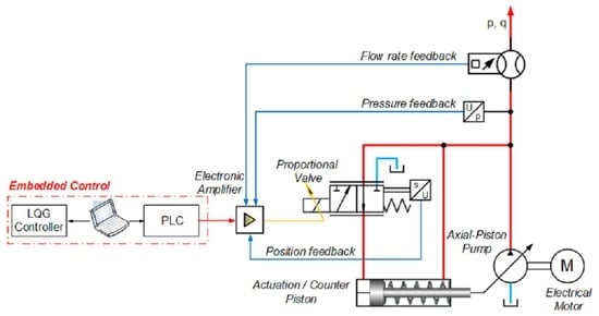
For the purpose of system identification and the subsequent development of embedded controllers, a laboratory test rig for the study of open circuit axial piston pumps with proportional valve control is developed and implemented [4]. The hydraulic circuit diagram of the test rig is shown in Figure 1, and its photo is presented in Figure 2. The system is based on a well-known model pump, A10VSO (Bosch Rexroth company). The regulation of the displacement volume of this type of pump is well known in the theory and practice of hydraulic drives [2]. It is based on two main approaches. The first consists of using a conventional hydraulic controller of type DR, DFR, DFLR, etc. These controllers are directly coupled to the pump casing and perform their regulating function (of pressure and flow rate) according to a certain law depending on their schematic and constructive solution. The other approach for their regulation consists of the use of a hydraulic valve that is specially developed for this type of pump with proportional electric control, which is mounted on the same plate of connection intended for the listed conventional controllers [21]. In this way, through integrated electronics or an external card type VT-5041, control of the spool of this valve is performed, and, in turn, the displacement volume of the pump is changed via the main energy parameters, pressure and flow rate [21,22]. In practice, this approach is designed to implement secondary control; however, it requires the use of a variant of the same pump that has a swash plate swivel angle sensor and the ability to change the angle of the swash plate in the opposite direction to work in the motor mode of operation. Inevitably, this modernization approach has a significantly higher cost but with an expanded range of applications. In this aspect, the developed control solution incorporates both regulation approaches. However, a pump is used without a swivel angle sensor and without the possibility of operation in motor mode. On the other hand, both types of controllers are used, connected in parallel by means of an additional developed mounting hydraulic block with a built-in check valve. It must be noted that this cannot be used for secondary control. Its advantage is that it can implement a hydraulic system with speed and load feedback based on a variable displacement axial piston pump of the most common type. A detailed description of the system was carried out in a previous publication [4]. Here, only a brief presentation is made, emphasizing the mentioned advantages and disadvantages compared to solutions imposed in practice.

As mentioned above, the system consists of a variable displacement axial piston type A10VSO designed for open-circulation hydraulic drive systems. The pump has an 18 cubic centimeters displacement volume. It is equipped with a hydraulic pressure controller whose designation is better known as DR. Parallel to it is a proportional hydraulic valve VT-DFP (Bosch Rexroth Company) designed only for this type of pump and having a built-in spool position sensor. Control of this type of valve is realized by a selective external electronic amplifier type VT-5041, of which only the valve spool position feedback function and the power stage are used to power its proportional solenoid [23]. Classically, the system structure is presented in Figure 3. In the developed solution, an electronic amplifier is used to receive a reference signal from a PLC MC012 [24]. The system software is distributed between the industrial controller and the desktop workstation to allow rapid prototyping of the different types of identification experiments and embedded controllers. This is another advantage of the system as it makes it possible to realize advanced control laws, not just conventional PID controllers and their varieties established in hydraulic drives. The distributed system is based on a real-time communication channel between the PLC and the workstation running a Simulink^® model (Mathworks). Communication is carried out via a USB/CAN network in blocking mode with a synchronization packet emitted from the industrial controller with a sample time of 10 milliseconds. This sampling period is fast enough to allow precise control of the pressure and flow rate.

3. System Identification

To employ the linear quadratic control method, a linear time-invariant state space representation of the axial piston pump is required. Generally, two approaches are available to build a state space model, either through the application of first principle physical laws [25] and the consecutive estimation of model parameters (“gray box” model), or alternatively, the application of “black box” system identification techniques [26,27]. The “gray box” approach requires a detailed understanding of the internal construction of the axial piston pump, as well as the exact measurement of geometrical and physical variables. Even though that approach is beneficial for advancing construction aspects of the axial piston pump machine by reaching a high-fidelity simulation model, it does not guarantee successful control system design. As we know, the purpose of control-oriented models is to focus on the numerical signal transformations between manipulated and performance variables because the controller will aim to invert these transformations in order to achieve the desired behavior of the system. Certainly, input–output transformation can be obtained from a high-fidelity physical model of the system; however, a lot of non-control-related information will also be incorporated into the physical model. Hence, considering the amount of effort and experimental work necessary to achieve precise physical modelling, in most situations, control engineers prefer the estimation of black box functional models. Additionally, digital controllers require discrete-time representation of the system dynamics, which can be naturally achieved by selecting a discrete-time structure for the representation of the black box model. The key elements in black box system identification are the model structure, identification experiment and estimation method.

For the purpose of axial piston pump control, the selected model structure is a discrete-time state space model in controllability canonical form (Cauchy representation):

$$x\left(k+1\right)=Fx\left(k\right)+Gu\left(k\right)+Ke\left(k\right),$$

(1)

$$y\left(k\right)=Cx\left(k\right)+Du\left(k\right)+e\left(k\right),$$

(2)

where $x={\left(x_1,x_2,\dots ,x_n\right)}^T$ is a state vector, $u\left(k\right)$ is the PWM signal applied to a proportional spool valve, $y={\left(y_q,y_p\right)}^T$ is the output signal, $y_q$ is the pump flow rate, $y_p$ is the pump pressure and $e={\left(e_q,e_p\right)}^T$ is the residual error with respect to pump flow rate ($e_q$) and $e_p$ pump pressure. $F,G,K,C,D$ are model parameters which are matrices with appropriate dimensions. To obtain model parameters, open loop identification experiments are performed for variable loading conditions according to the scheme presented in Figure 4. The discrete-time experiment is carried out with sample time $T_s=0.01 \mathrm{s}$, which is sufficiently small for this type of dynamic system. The identification input signal is a white Gaussian noise that is applied as a PWM voltage signal to a proportional valve.

The measured output signals are pump flow rate and pump pressure. The date set obtained after the experiment in the presence of full loading (the loading throttle valve depicted in Figure 1 is approximately close) is depicted in Figure 5, Figure 6 and Figure 7.

The first 1000 points are removed from the data set in order to exclude transient responses. The remaining data are centered and divided into two data sets, the first is used for parameter estimation, and the second is used for model validation. Due to the absence of accurate information for the order of models (1) and (2), the models of the 1st to 10th order are estimated.

The Hankel singular values of models from the 1st to 10th order are depicted in Figure 8. As can be seen from the figure, the appropriate model order is the 5th, but the model of the 6th order has singular values close to the ones of the 5th order model. The Hankel singular values test provides only initial information about the supposed model order and cannot be used alone to determine the appropriate model. Thus, the models of the 4th, 5th, 6th and 8th orders are estimated. The comparison of measured outputs and those simulated by estimated model outputs are presented in Figure 9. As can be seen from the pump flow rate, the FIT between the measured and simulated signals is almost the same for all models. However, for the pump pressure, the FIT between the measured and simulated signal for the models of the 5th, 6th and 8th orders is significantly large compared to the one for the 4th order model.

The models of the 5th, 6th and 8th orders passed residual correlation tests (Figure 10). As can be seen, the residual error for both outputs is white Gaussian noise. This indicates that the obtained parameter’s estimates are unbiased. Additionally, the residual error is uncorrelated with input signals which shows that the model sufficiently describes the pump dynamics for both channels.

The 6th order is most appropriate due to the fact that it also has good performance in the case of non-loading conditions (the loading throttle valve is fully open). This can be seen from the frequency responses of estimated models in non-loading conditions, which are depicted in Figure 11. It is seen that in a high-frequency range, the responses of the 6th and 8th model orders are close, whereas the response of the 5th order model is approximately the same as the 4th order model.

The step responses along their confidence intervals with respect to pump flow rate and pump pressure for the 4th and 6th model orders are depicted in Figure 12. It is seen that the confidence intervals are small.

The matrices of the estimated 6th order model take the values:

$$\begin{gathered} \mathrm{A}=\left(\begin{array}{cccccc}0& 1& 0& 0& 0& 0\\ 0& 0& 1& 0& 0& 0\\ -0.3& 0.43& 0.84& -0.01& 0.04& -0.03\\ 0& 0& 0& 0& 1& 0\\ 0& 0& 0& 0& 0& 1\\ 0.57& -11.17& 10.83& 0.72& -1.62& 1.9\end{array}\right), \mathrm{B}=\left(\begin{array}{c}0.005\\ 0.161\\ 0\\ 0.209\\ 0.046\\ 0.058\end{array}\right), \\ \mathrm{K}=\left(\begin{array}{cc}0& 0.075\\ 0.082& -0.015\\ 0.031& 0.031\\ 0.423& 0.099\\ -0.033& 0.259\\ 0.141& -0.029\end{array}\right), \mathrm{C}=\left(\begin{array}{cccccc}1& 0& 0& 0& 0& 0\\ 0& 0& 0& 1& 0& 0\end{array}\right) \mathrm{and} \mathrm{D}=\left(\begin{array}{c}0\\ 0\end{array}\right). \end{gathered}$$

(3)

4. LQG Control Design

The structure of the designed control system is depicted in Figure 13. The purpose of the controller design in this research is to regulate the flow rate $y_q$ of the axial piston pump to the desired reference value $r_q$ with maximal steady-state accuracy and minimal settling time. Several problems arise in the control of axial piston pumps. First, the pump is based on a single input multiple output (SIMO) model. It can be established through the controllability test that we can regulate both pressure $y_p$ and the flow rate $y_q$ to desired values, if and only if they lie in a common equilibrium manifold $y_p=f\left(y_q\right)$. However, due to the uncertainty in the system dynamics, the exact analytical form of the manifold is not established; hence, we can either regulate the pressure or the flow rate alternately. The second problem arising from the control design is the inherent uncertainty in the identified pump model. This uncertainty can be characterized by the limited size of the identification data, the presence of uncontrollable disturbances acting on the plant and the non-stationarity of the pump dynamics with the selected operating point. The operating point is selected in our experiment by the level of closing of the precise resistance throttle valve bypassing the pump. Hence, the third problem with the present system is that due to uncertainty, it requires a feedback controller. However, due to the static nature of the plant model, we need to extend the feedback loop with an additional integrator element to guarantee reference tracking in the presence of output loading disturbances.

The linear quadratic control approach is derived from the key results of optimal control theory, where a quadratic cost functional is minimized with respect to the realization of the control signal. The benefit of the LQR optimal solution is that it can be represented as a function of the Lagrange multiplier costate vector which is coupled to the system state vector through the solution of the differential Ricatti equation [28]. The quadratic cost function for the closed-loop pump model is selected as

$$J\left(u\right)={\displaystyle \sum }_{k=0}^{\infty }{\mathit{x}}^T\left[k\right]Q_x\mathit{x}\left[k\right]+ru{\left[k\right]}^2+w_{I_y}{I}_y\left[k\right],$$

(4)

where $\mathit{x}\left[k\right]={\left(\begin{array}{cccccc}{\mathit{x}}_q\left[k\right]& {\mathit{x}}_2\left[k\right]& {\mathit{x}}_3\left[k\right]& {\mathit{x}}_p\left[k\right]& {\mathit{x}}_5\left[k\right]& {\mathit{x}}_6\left[k\right]\end{array}\right)}^T$ is the state vector of the identified pump model, $Q_x\in {ℝ}^{6\times 6}$ is the positive definite real matrix weight of the state vector components and their correlations and $r\in ℝ$ is the weight gain for the amplitude of the control signal. In the cost function, we also include the signal $I_y\left[k\right]$ weighted with $Q_y\in ℝ$, which represents the integrated output error with respect to the flow rate:

$$I_y\left[k\right]={\displaystyle \sum }_{i=0}^k{T}_S\left(r_q\left[k\right]-y_q\left[k\right]\right)={\displaystyle \sum }_{i=0}^k{T}_S{e}_q\left[k\right].$$

(5)

For calculation purposes, the integrated signal is represented as a finite difference equation for a first-order Euler approximation of the integration operation in continuous time as

$$I_y\left[k\right]=I_y\left[k-1\right]+T_S{e}_q\left[k\right].$$

(6)

The weighting matrix $Q_x$, together with $r$ and $w_{I_y}$, are tunable parameters reflecting performance requirements for the closed-loop system. However, due to the implicit representation of the physical state variables in the state vector, it is not obvious how to select the components of the matrix $Q_x$. Hence, we employ mapping with matrix $C$ between the output and the state variables to translate the tuning of $Q_x$ into the output space as

$${\mathit{y}}^T\left[k\right]Q_y\mathit{y}\left[k\right]={\mathit{x}}^T\left[k\right]\left(\begin{array}{cc}{C}_q{}^T& 0\\ 0& C_p{}^T\end{array}\right)Q_y\left(\begin{array}{cc}{C}_q& 0\\ 0& C_p\end{array}\right)\mathit{x}\left[k\right]={\mathit{x}}^T\left[k\right]Q_x\mathit{x}\left[k\right],$$

(7)

where the matrix $Q_y\in {ℝ}^{2\times 2}$ is a corresponding weighting matrix in the output space of the model. Since the physical meaning of the output signals is established as $y={\left(\begin{array}{cc}{y}_q& y_p\end{array}\right)}^T$, we can specify the matrix $Q_y=diag\left(w_q,w_p\right)$, where $w_q$ represents the cost weight for the flow rate channel and $w_p$ represents the cost weight for the pump pressure channel. In this mapping, the matrix

$$Q_x=\left(\begin{array}{cc}{C}_q{}^T{w}_q{C}_q& 0\\ 0& C_p{}^T{w}_p{C}_p\end{array}\right).$$

(8)

Considering that in the identified model, matrices $C_q$ and $C_p$ contain just one non-zero element, i.e., a unit corresponding to the state for the output signal, we see that with such a weighting matrix, we put weight on only two of the states and the rest are left outside of the cost function, or we do not care for their amplitude, since they do not carry an explicit physical meaning.

Equivalently, we can extend the state vector of the plant model, including the integrator state $I_y\left[k\right]$, as

$${\mathit{x}}_{\mathit{e}\mathit{x}\mathit{t}}=\left(\begin{array}{c} I_y\\ \mathit{x}\end{array}\right),$$

(9)

and then the plant model matrices $F$ and $G$ will become

$$F=\left(\begin{array}{ccc}1& -T_S{C}_q& 0\\ 0& F_q& F_{qp}\\ 0& F_{pq}& F_p\end{array}\right),G=\left(\begin{array}{c}0\\ G_q\\ G_p\end{array}\right).$$

(10)

Additionally, the state weighing matrix for the extended state vector will become

$$Q_{ext}=\left(\begin{array}{cc}{w}_{I_y}& 0\\ 0& Q_x\end{array}\right).$$

(11)

Following the methodology for LQR design, we look for a linear state feedback controller gain such that the control signal is

$$u\left[k\right]=-K_p\mathit{x}\left[k\right]+k_i{e}_q\left[k\right]=-K_{ext}{\mathit{x}}_{\mathit{e}\mathit{x}\mathit{t}}\left[k\right],$$

(12)

where $K_p\in {ℝ}^{1\times 6}$ is a row vector with proportional gains multiplying the state vector, and $k_i\in ℝ$ is the integral gain multiplying the reference tracking error $e_q\left[k\right]$ for the flow rate, then $K_{ext}=\left(\begin{array}{cc}{k}_i& K_p\end{array}\right)$. According to ref. [28], these gains can be obtained as

$$K_{ext}=\frac{G^{T}PF}{G^{T}PG+r},$$

(13)

where the denominator is scalar because the system has a single input. The matrix $P$ is a positive definite solution of the infinite time algebraic Ricatti equation

$$F^{T}PF-P-F^{T}PG{\left(G^{T}PB+r\right)}^{-1}{G}^{T}PF+Q_{ext}=0.$$

(14)

The numerical values we select for the integrated error $w_{I_y}=500$, the flow rate channel $w_q=0.001$, the pump pressure $w_p=0.001$ and the control signal amplitude $r=0.001$ lead to the following solution for the state feedback

$$k_i=637.7478,$$

(15)

$$K_p=\left(-1.27,19.9,28.91,-0.88,1.77,-0.92\right).$$

(16)

As can be seen, the integral gain of 637 dominates the controller response, followed by the gain of 28.9 for the third state variable, representing the delayed flow rate output $y_q\left[k-2\right]$, followed by the gain of 19.9 for the $y_q\left[k-1\right]$.

The key problem with the practical implementation of the LQR controller is that the internal state vector of the system $\mathit{x}\left[k\right]$ is generally inaccessible for direct measurement. Hence, it must be estimated by a calculated value $\widehat{\mathit{x}}\left[k\right]$ from the previous values of the measurable system signals (the input and output plant channels). To produce the state vector estimate, we employ the stationary Kalman filter algorithm, which minimizes the variance $E\left({\left(\mathit{x}\left[k\right]-\widehat{\mathit{x}}\left[k\right]\right)}^2\right)$ of the estimation error over all initial conditions and realizations of the model residuals $e_q\left[k\right]$ and $e_p\left[k\right]$, which are assumed to behave as Gaussian white-noise processes with unit variance. In addition, an unbiased estimate is usually required, meaning

$$E\left\{\widehat{\mathit{x}}\left[k\right]\right\}=E\left\{\mathit{x}\left[k\right]\right\}.$$

(17)

The Kalman filter algorithm has many modifications [29] depending on the model of the process and the assumptions about the statistical distribution of the noise and disturbances. The model of the axial piston pump is a linear time-invariant system with stationary noise action on the state and output. Hence, we design the state observer algorithm as

$$\widehat{\mathit{x}}\left[k+1\right]=F\widehat{\mathit{x}}\left[k\right]+Gu\left[k\right]+L\left(\mathit{y}\left[k+1\right]-CF\widehat{x}[k]-CG\widehat{x}[k]\right),$$

(18)

where $L\in {ℝ}^{6\times 2}$ is the filter gain matrix calculated to minimize the state error variance. The filter gain is calculated as

$$L=D{C}^T{\left(CD{C}^T+0.01I_2\right)}^{-1},$$

(19)

where $V_e=E\left(e{e}^T\right)\in {ℝ}^{2\times 2}$ is the variance of models’ (1) and (2) residuals, and $D$ is the error covariance matrix calculated as a solution of the algebraic Ricatti equation,

$$D=F{D}_e{F}^T+K{V}_e{K}^T.$$

(20)

The resultant filter gain matrix obtained from the identified model becomes

$$L=\left(\begin{array}{cc}0& 0.07\\ 0.08& -0.02\\ 0.03& 0.03\\ 0.42& 0.1\\ -0.03& 0.26\\ 0.14& -0.03\end{array}\right).$$

(21)

The first column from the filter gain matrix corresponds to the flow rate channel and the second column corresponds to the pressure output signal. The filter gain depends on how much information is carried from each state to the output signal and how much we can trust the output signal given the present level of external noise variance. Therefore, the higher gains in matrix $L$ indicate that the respective state variable will be more strongly compensated by the output estimation error. The optimal error covariance matrix obtained from the solution of the Ricatti equation is

$$D={10}^{-4}\times \left(\begin{array}{cccccc}2& 0& 1& -2& 2& -1\\ 0& 2& 1& 3& -1& 0\\ 1& 1& 1& 0& 0& 0\\ -2& 3& 0& 40& 11& 13\\ 2& -1& 0& 11& 24& 12\\ -1& 0& 0& 13& 21& 21\end{array}\right).$$

(22)

As can be seen from the diagonal elements, the variance of the first three states determining the flow rate output signal of the model is 10 times lower than the variances of the pressure determining states. The same is true for the cross-correlations between the errors of the estimated states. The fundamental mechanical constraints can explain that in the pump, when provided with a fixed input signal to the proportional valve, the swash plate swivel angle will determine a fixed displacement volume leading to a fixed flow rate in dependence on the shaft rotation speed. On the other hand, the pressure in the system will be more strongly dependent on the externally attached loading system to the pump and not so much on the input signal $u\left(t\right)$. Hence, the variance in the estimated pressure states will become higher. Another observation from the state covariance matrix is that the 3rd and 6th states have lower variances than the 1st and 2nd or 4th and 5th states. This can be related to the casual relationships between those states if one observes the structure of matrix $F$.

Figure 14 presents the closed loop system frequency responses with the designed linear quadratic regulator and Kalman filter. The output sensitivity function characterizes the ability of the closed loop to attenuate the loading disturbances. We see that the designed regulator dampens the amplitudes of the output disturbances up to 100 times in the low-frequency domain and around 10 times in the middle frequency up to 2 rad/s. From the complementary sensitivity function, we can say that the bandwidth of the closed loop is around 10 rad/s which is acceptable for a regulated pump, considering the capabilities of the employed actuator and flow meter. Figure 14 also shows the control signal sensitivity. As expected, it is higher in the low-frequency range and lowers down in the high frequencies to prevent amplification of measurement noise in the actuator command.

5. Experimental Validation of Designed Controller

This section presents the experimental results measured with the designed controller in a hardware in the loop (HIL) experiment with the MC012 microcontroller. The loading system for the pump is represented by a variable throttle valve bypassing the output of the pump to the tank, which is presented in the hydraulic circuit diagram in Figure 1. The opening of the loading throttle valve can be manually selected by a precision micrometer scale from 0 to 5 mm. We test the performance of the LQG controller for loading throttle valve openings of 2 mm, 3 mm, 4 mm and 5 mm. The recorded signals are the output pump pressure, output flow rate, LVDT feedback from the pump proportional valve and control signal sent to the electronic amplifier. The experimental results are summarized in Figure 15, Figure 16, Figure 17 and Figure 18.

For the minimal opening of the loading valve of 2 mm, the closed loop pump system will experience maximal loading as pressure. In such conditions, the reaction force on the swash plate from the output pressure will be maximal, and the control effort from the actual will be required to compensate for the variations in the flow rate. To examine the system during such conditions, we apply a reference flow rate of 14 L per minute and a step reference jump to 17 L per minute for a period of 2.5 s. As can be seen in the figure, we note a very fast system response below 100 ms. The flow rate is held around the reference value with random deviations of +/− 0.5 L per min. Part of these observed variations can be attributed to the sensor noise and imprecision. As noted in the introduction, we employ a low-cost flow rate meter based on an orbital hydraulic motor and a hall sensor. Measurement is based on the capturing of the impulses period from the Hall sensor with a precision of 100 ns. Hence, this measurement technique will introduce some limitations to the maximal accuracy we can obtain for the flow rate. Another component of the observed flow rate variations can be attributed to the actual irregularities in the flow through the gear flow meter. During these high loading experiments, we observe very demanding conditions for the system with pressure in the range of 80 to 120 bar, providing a power output of around 2 kW. Since the electrical motor driving the pump shaft is an unregulated three-phase induction machine, such a high load will lead to variation in the rotational speed of the motor, reflecting directly on the generated flow rate by the pump. Even in such high loading conditions, the designed control system is able to keep the mean value of the flow rate signal around the reference value without much amplified noise in the control signal.

Figure 16 examines the transient behavior for lower loading corresponding to the opening of the loading throttle valve of 3 mm. The pressure during this experiment is around 50 bars, which corresponds to the output power of the pump of around 1.5 kW. The reference signal of the controller is a step from 19 L per minute up to 24 L per minute. The transient response and accuracy of the regulations are comparable to the case of a 1.5 kW operating point with a settling time below 100 ms. It is interesting to note that with an increase in flow rate through the pump, increasing the pressure and the output power, the amplitude of flow rate variations increases. This can be taken as a confirmation of the hypothesis that flow rate variations are due to increased load on the induction motor causing the instability of its rotational speed.

Figure 17 examines the reference tracking performance for the case of a 4 mm opening of the loading throttle valve. In this case, we set the reference step levels between 21 L/min and 26 L/min. The operating pressure in these conditions is between 20 to 30 bars, providing a power output for the pump of around 1 kW. In these conditions, the settling time is increased to around 100 ms. Due to decreased pressure in the system, the reaction of the swash plate to change in the actuating piston becomes slower; hence, the transient responses are delayed. However, such a scale of the response is within sufficient limits for the practical application of the controller. The flow rate variations, in this case, are comparable to the case with the opening of the loading valve up to 3 mm. Similar to the previous case, the amplitude of the variations increases with the increasing flow rate, hence the increased power output of the pump.

The last examined loading condition (Figure 18) corresponds to a 5 mm opening of the loading valve, which can be characterized as minimal loading. During the experiment, the reference step is from 22 L per minute to 27 L per minute. The settling time is around 200 ms, which again is increased because of the decrease in the pressure in the system, reducing the forces acting on the action valve to move the swash plate. It is worth noting that, in these cases of loading, minimized variations of the stationary flow rate around the reference are observed. The pressure in the system is around 20 bar which corresponds to power output below 1 kW. In this case, the loading of the induction motor driving the pump is reduced, and its rotation speed is more stable, which minimizes the variations in the flow rate.

Experimental results for the flow rate regulation prove the experimental stability and performance of the designed LQG controller. The controller is examined for four operating points in the full range of loading conditions for the pump between 14 to 26 L per minute. Even though the identified model is for a single operating point, the closed loop system is able to maintain the reference tracking performance, which is an indication of its robustness.

Figure 19 compares the resultant pressures in the system for the four operating points selected by opening the loading throttle valve. As can be expected with the increase in flow rate, the pressure in the system is increased too. It is notable that for the highest loading conditions, the oscillations in pressure are much more pronounced. Hence, it is not recommended to operate the closed loop system at such high pressure for prolonged intervals. The working envelope of the designed closed loop system can be characterized by a flow rate range between 14 and 26 L/min and a pressure range between 20 to 80 bar. Another thing which can be noted in the figure is that there is a nonlinear relationship between the opening of the loading valve and the mean value of the pressure in the system.

Figure 20 shows the control system from the LQG controller during the experiments. The control signal sent to the valve is from 0 to 10V. Therefore, the negative values in the figures are saturated at 0. The most important feature of the examined control signals is that they do not amplify the sensor noise present in the output. This is because of the application of the noise model from the system identification and because of the design of the Kalman filter. Such output noises can be easily amplified by some classical control algorithms, such as PID, leading to the overloading of the actuator valve. It is interesting to note that the average value of the control signals for the selected operating points is not much different, which is an indication that the identified model is able to carry information not only for its operating point but for others too.

Additionally, in Figure 21, we present the LVDT signal for the proportional valve position during the examined loading conditions. The valve we use is bidirectional; hence, we limit its range from 0 to 50% because in the pump we test, the swash plate can work only on positive swivel angles. Alternatively, if the pump can be inverted to work as a motor, the proportional valve operating range will be from 0 to 100%. In the figure, it is important to note that the proportional valve is fast enough to follow the dynamics of the generated control signal from the controller.

As an additional experiment, we examine the performance of the pump for a fixed reference flow of 22 L per minute and with variable (dynamic) loading conditions simulating a real application operation. The loading is modeled by manually decreasing the opening of the loading valve from 5 mm to 1 mm. Figure 22 and Figure 23 present the results of this experiment. As can be seen in Figure 22, the flow rate is held steady by the control system at 22 L/min for all loading pressures in Figure 23 from 20 to 100 bar. With the increase in the loading of the pump and the required output power from the induction motor, the oscillations in the flow rate begin to increase too.

6. Conclusions

The main contribution of the article is the developed embedded system for control of an axial piston pump with a proportional valve. In contrast with existing solutions, in this work, the developed embedded system uses a pump that is not equipped with a swash plate swivel angle sensor and rotational speed sensor. This solution is not appropriate for secondary control but is appropriate for flow and pressure control of open-circuit hydraulic drive systems. The proposed control solutions provide possibilities to implement not only existing analogue PID controllers but also advanced control algorithms. First, the “black box” model of the axial piston pump with proportional valve control is estimated from experimental data. The results of validation tests show the model accuracy and its applicability for controller design. The designed control system is based on a linear-quadratic Gaussian (LQG) controller with a time-invariant Kalman filter that is implemented on a laboratory test rig. A detailed description of the hydraulic system in the context of pump displacement control is presented, as well as the developed system architecture for its control. The designed control system is validated through experimental studies for various loading conditions that enable the analysis of its performance.