Abstract
The automated evaluation of machine conditions is key for efficient maintenance planning. Data-driven methods have proven to enable the automated mapping of complex patterns in sensor data to the health state of a system. However, generalizable approaches for the development of such solutions in the framework of industrial applications are not established yet. In this contribution, a procedure is presented for the development of data-driven condition monitoring solutions for industrial hydraulics using supervised learning and neural networks. The proposed method involves feature extraction as well as feature selection and is applied on simulated data of a hydraulic press. Different steps of the development process are investigated regarding the design options and their efficacy in fault classification tasks. High classification accuracies could be achieved with the presented approach, whereas different faults are shown to require different configurations of the classification models.
1. Introduction
Over the lifetime of an industrial machine, wear and tear of various components of the system is inevitable. Especially in applications that involve the transmission of high power under rough conditions, as typically present in hydraulics, the health state of machine elements will degrade over time. In order to maintain high machine availability and process quality, maintenance actions are required. However, the task of planning maintenance actions can be challenging for machine operators when a balance must be met between premature downtimes due to maintenance work and downtimes due to decreased process quality or machine damage. To plan maintenance periods efficiently and detect looming failures at an early stage, methods of condition monitoring can be applied. The objective of condition monitoring is to obtain an estimate of the current machine health status through the automated evaluation of operation data gathered from a machine [1].
In the field of hydraulics, different approaches for condition monitoring have been investigated. Solutions studied and suggested in the literature range from rule-based systems to model-based approaches, to purely data-driven approaches [2,3]. Most recently, the increasing integration of measurement technology and information technology in industrial products [4] turned the focus to another group of methods, the data-driven approaches. These methods, often summarized by the term machine learning, aim to algorithmically extract a model from data, which maps patterns in recorded data to corresponding machine health statuses. In the case of methods of supervised learning, the health state of a machine can be determined based on the algorithmic processing of observed sets of sensor and control signals [5]. Moreover, given the labeling of the data, the cause of deviating machine behavior can even be traced down to faults in the components of the system.
However, challenges in the application of data-driven approaches for condition monitoring still exist. One major issue is the lack of methods for the general and generic development of data-driven solutions. Another challenge is the requirement of comprehensive data. To obtain robust models, the training data used should cover a broad range of possible operating scenarios and machine configurations. Additionally, machine learning-based approaches are regarded as black-box models, which hardly provide human inspectors an insight into the process of decision making learned by such models [6].
In this contribution, a method for developing data-driven condition monitoring solutions for industrial hydraulics is presented. For this, a feature-based approach of supervised learning is applied, which allows the generic extraction of features from multivariate, cyclic and non-stationary time series data. Moreover, the presented procedure includes a feature selection step, which helps in identifying relevant data characteristics and gives an insight into the effect of faults on observable measures of the system. For the setup and training of classification models, a flexible approach is suggested, which allows the modular setup of classification models for individual machine and component faults. Investigations are carried out on a simulation model of a hydraulic press test bench, such that the issue of data availability is not a limiting factor in this study.
2. Related Work and State of the Art
In this section, an overview of previous work on condition monitoring in hydraulic applications is given. Subsequently, the general concept of neural networks is described with respect to relevant design aspects for the setup and use in a fault classification solution.
2.1. Condition Monitoring in Hydraulics
In general, applying machine learning for the condition monitoring of hydraulic applications has proven to yield satisfactory results [2,7,8]. Most publications in this field focus on the use of data-driven techniques for monitoring single hydraulic components such as pumps and valves [9,10,11,12]. The algorithms mainly used in these studies are based on variations of neural networks, which are used to process raw time series for the inference of the health states of the components. In [13], features are extracted from the raw time series in order to detect anomalies in the operation of a speed-variable pump by the use of methods of unsupervised learning. A similar feature-based approach is pursued in [14] in the framework of a systematic investigation of techniques of supervised learning for monitoring an axial piston pump. As typically only a few sensors are applied at the component level, data are scarce in these use cases, such that mostly only one single sensor recording can be considered. On the contrary, applying condition monitoring on a system level enables to include further sensor data available in the system. Hence, a component fault cannot only be inferred directly from data acquired on that component, but can also be inferred from indirect effects on other components and the overall system behavior. This concept is successfully applied in [15,16] for hydraulic system test benches by also using a feature-based approach. The features mostly used are measures from descriptive statistics, such as the mean, median and variance of a signal, while, for rotating machinery, features from the frequency domain are often considered [15]. Alternatively, features can be manually defined, as in [17]. In [18], the authors have investigated refinement strategies of generic feature generation, where including process knowledge into the feature generation was shown to improve the detection of faults. Furthermore, in [14] and [16], a feature reduction is performed by applying filter methods and analytical methods of principal component analysis, respectively. While a significant reduction in features can be achieved with a principal component analysis or a linear discriminant analysis, the resulting feature sets are not interpretable by a human inspector after the transformation [19].
2.2. Design Considerations for Neural Networks
In contrast to conventional approaches, data-driven methods depend less on domain-specific knowledge but extract the knowledge implicitly or explicitly from data. In the field of machine learning, this process of knowledge extraction is referred to as model training, where the model is a mathematical structure that is fit to reproduce a desired input–output behavior. The type of model mainly considered in this study is feedforward neural networks in the form of multilayer perceptrons, as shown in Figure 1.
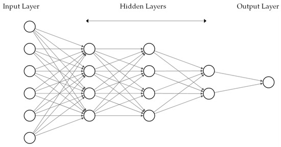
Figure 1.
Feedforward neural network with sic nodes in the input layer, three hidden layers and one node in the output layer.
Feedforward neural networks consist of neural units sequentially stacked in layers, where the outputs of a preceding layer form the inputs for the subsequent layer. In regular fully connected neural networks, the outputs of all units of a preceding layer are connected to each neural unit of the next layer, where each connection is attributed a weight parameter. Within the units, the respective input values are multiplied with the corresponding weight parameter, summed up and passed through an activation function. The main purpose of the activation function is applying a transformation to the data between the layers and using nonlinear activation functions to enable nonlinear mappings between input samples and the output of the network [20]. Accordingly, typically used activation functions are the sigmoid activation function, tanh activation function or a rectified linear activation function (ReLU).
The layers located between the input layer and the output layer of the network are referred to as hidden layers. Theoretically, using one hidden layer with a nonlinear activation and an arbitrary high number of nodes in the hidden layer allows to approximate any given input–output relationship [21]. Accordingly, combining multiple layers linearly, as done in a multilayer perceptron, preserves this characteristic of a universal approximator. Moreover, combining multiple layers adds to the representational capacity of a neural network, which, in turn, can allow to use less nodes in the network in total compared to the network with a single hidden layer [20].
In order to obtain a desired input–output mapping from a neural network, the weight parameters of the model are adjusted algorithmically during the model training. For this, each training sample is first passed to the input of the model in a forward pass, where the model outputs a value. After this, the deviation between the model output from the forward pass and the desired output is computed according to a predefined loss function. Subsequently, in the reverse pass, the gradient of the loss function is computed with respect to the model weights, so that it can be inferred which model weights to adjust in order to minimize the loss. While the reverse pass is performed by generic gradient-descent-based algorithms, the selection of the loss function is linked to the format of the model output of the model, i.e., whether continuous values or discrete class labels are predicted [22]. In contrast to the weight parameters of the model, the structural parameters (number of layers, number of nodes and activation functions) and fitting parameters (loss function and optimization algorithm) remain fixed during training. Therefore, these parameters are referred to as the hyperparameters of a model. Applying neural networks hence requires to define these hyperparameters for the specific problem at hand. As no general rule exists for setting the hyperparameters of neural networks, especially for the structural hyperparameters, they are often determined based on experience or by implementing and comparing several setups. The latter approach is also referred to as grid search.
Furthermore, methods of supervised learning are based on fitting models to training data, for which the expected output of the model is known. In the case of condition monitoring, this can be any indicator of the machine health status, which, in turn, can be represented by a single value or be composed of multiple values. The former, the single-value case, is referred to as single-target prediction, while the latter case is referred to as multi-target prediction. Furthermore, in the case of classification, where the task is to predict discrete classes for a set of inputs, a distinction can be made based on the number of possible classes that each target can represent. In the most basic case, targets are binary values, but cases of multiple classes are possible as well.
2.3. Feature Representation of Time Series Data
As the number of input nodes of a neural network is fixed, the dimensionality of the input data must be uniform among all data instances, too. However, time series data, as typically acquired from sensors in industrial machines, can have varying lengths, depending on variations in the process or the sampling rates of different sensors. Moreover, the longer the time series, the more input nodes are required, and the number of parameters of the neural network unfavorably increases. Therefore, describing a time series by a fixed number of representative characteristics is one common means to obtain the compatibility of time series and a fixed number of model inputs [22]. These characteristics are referred to as features and can be either defined manually [19], by the use of generic descriptive measures [23], or derived by transformation of the data learned by another machine learning model [24].
3. Materials and Methods
In this section, the considered hydraulic system is described and the developed approach for generating fault classification models is presented. This includes the steps of data generation, feature extraction and selection, as well as the process of model setup, training and evaluation.
3.1. Hydraulic Press
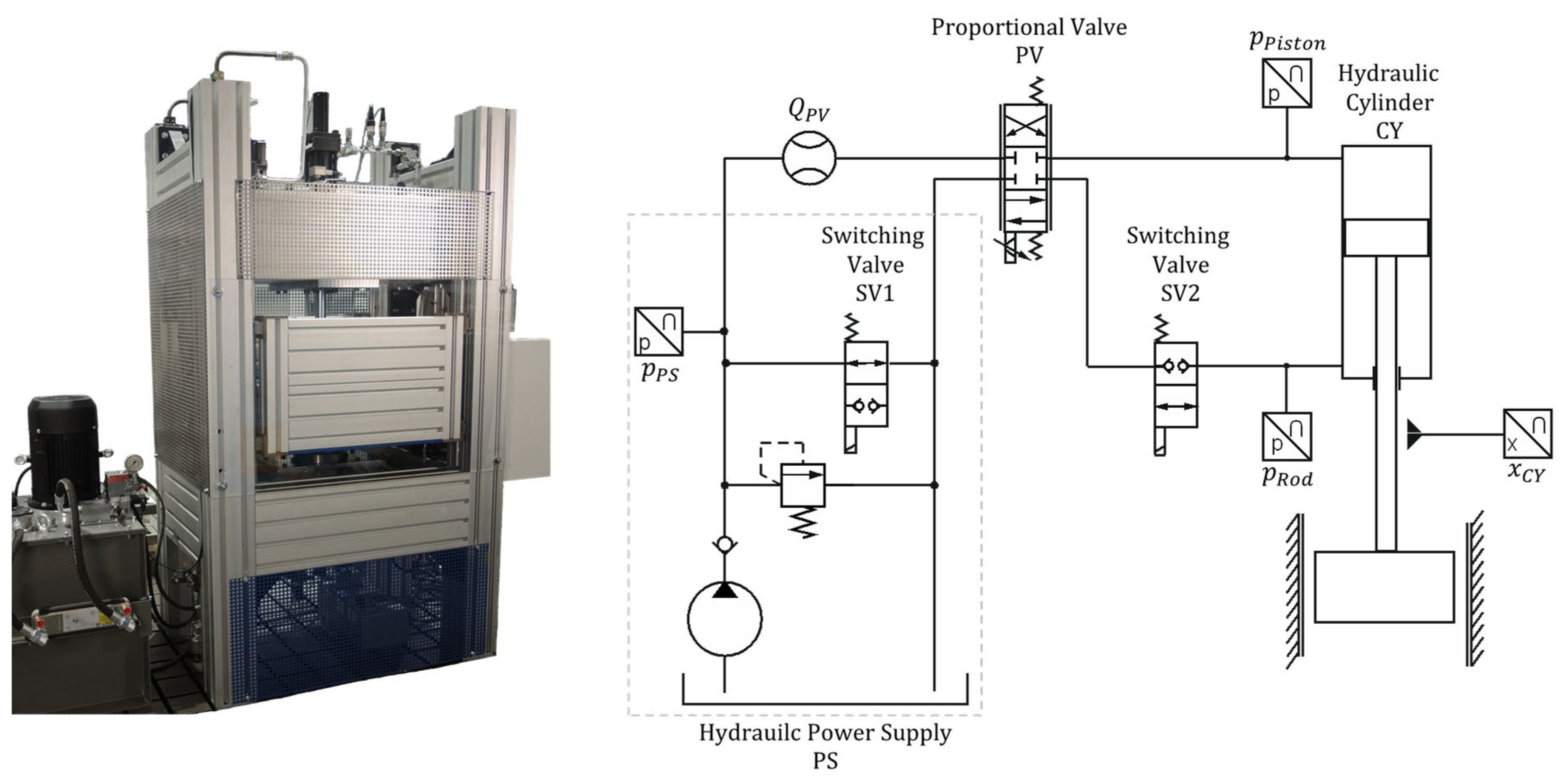
Representative of an industrial hydraulic system, a hydraulic press is considered in this study. Figure 2 shows the physical machine, along with the corresponding hydraulic circuit diagram. The system mainly comprises a position-controlled cylinder drive. The hydraulic power is supplied by a pump and conducted to the double-acting hydraulic cylinder (CY) through a proportional 4/3-way directional control valve (PV). Two switching valves (SV1 and SV2) allow to set the system to idle circulation and to lock the ram in position, respectively. The pump provides a constant volumetric flow of approximately 19 L/min at a maximal system pressure of 200 bar. The hydraulic cylinder has a nominal piston diameter of 80 mm and is coupled to a guided ram, which finally acts against a load force. The load force represents the reaction force of a workpiece and is provided by a secondary circuit in the physical test bench. During operation of the press, pressures are measured at the main cylinder and the power supply. Additionally, the position of the cylinder is recorded, as well as the volumetric flow entering the 4/3-way directional control valve and the control signals fed to the valves.
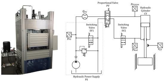
Figure 2.
Hydraulic press test bench and its hydraulic circuit diagram.
The function of the system is to perform working cycles, in which the ram is moved to a defined position against the load force. At the beginning of the working cycle, the system is in idle mode, where the switching valve SV1 activates idle circulation of the pump and the switching valve SV2 locks the ram in the top position. Then, starting from the top position, SV1 and SV2 are switched and the main cylinder extends towards the workpiece in rapid traverse. During this phase, neither an external load nor a limitation of the velocity is active. As the ram approaches the workpiece and reaches a defined distance from it, the velocity is restricted through limiting the control signal of the valve PV and the volumetric flow to the cylinder, respectively. As the ram is in contact with the workpiece, an external load acts against the cylinder and increases linearly over the stroke of the cylinder. In this load phase, the system is given a fixed time to reach the set value, which depends on the desired target position of the ram. After this time, the controller initiates the backstroke in open-loop control and the cycle ends with another idle phase. Figure 3 shows the progression of cylinder position, velocity and load force over one working cycle of the press.
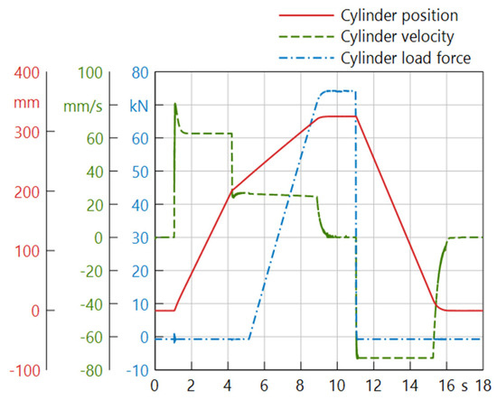
Figure 3.
Simulated working cycle of the hydraulic press in regular operation.
For the generation of the large amounts of data required in this study, a corresponding simulation model of the system is set up as a lumped parameter model using the simulation software SimulationX (software version 4.2) [25]. Hydraulic components in the simulation model are parametrized according to nominal data sheet specifications. The pump is modeled with a pressure-dependent volumetric loss, while no information on hydro-mechanical parameters could be derived from the pump data sheet. Furthermore, the dynamic characteristics of the pump and the driving electric motor are neglected. A linear opening characteristic is defined for the proportional valve, while the relationship between the spool position and control signal is modeled by a second-order differential equation. Pressure losses in the piping are neglected. However, the capacitance of conductors is considered where hoses or long pipes are installed in the real system. This is especially the case for the hosing and piping from the hydraulic power supply to other parts of the system.
To enable the effective training of a fault classification model from data, the training data ideally comprise all possible cases of operating scenarios and fault conditions. Hence, besides the regular operation of the press, operation under fault conditions must be emulated in the simulation model as well. Here, faults are emulated by introducing fault models into the lumped parameter simulation, which then are adjusted in intensity by varying the parameters of the fault models. The considered component faults are listed in Table 1. Leakages at the cylinder are modeled as pressure- and velocity-dependent flow through circular gaps, while the leakage at a connector of the hydraulic power supply is modeled by a pressure-dependent leakage factor. Increased friction at the main cylinder is modeled as an increased friction level, which is adjusted by setting the static friction force, whereas the dynamic friction force is lower than the static friction force by a constant factor. A worn valve spool is modeled by the valve spool overlap, while a sensor offset fault is introduced by adding an offset to the true sensor value. More detailed descriptions of the fault models used are given in [26].

Table 1.
Faults of the hydraulic system considered in this study, along with the corresponding model parameters of the simulation model and their ranges of variation.
3.2. Data Generation and Labeling
A dataset is generated from the simulation model by means of a variational study, where model parameters are varied. For this, a sampling scheme must be defined for the variable parameters of the simulation model. Here, the basis of the sampling scheme is a Latin Hypercube design. It is generated by creating ten random sampling schemes and choosing the design that best fulfills the maximin criterion. Accordingly, the scheme with the largest minimal distance between samples in the parameter space is selected. The eight-dimensional parameter space is formed by the six fault-indicating parameters and two process parameters, namely the target position of the press and the load force. Both process parameters are varied in three different levels of 290 mm, 310 mm and 340 mm and 40 kN/mm, 60 kN/mm and 80 kN/mm, respectively. Hence, in the obtained dataset, different fault intensities, fault combinations and operating conditions are represented. The temperature, however, is kept constant at 40 °C in all simulation runs.
While a Latin Hypercube design generally aims at sampling uniformly from the parameter space, different regions in the design space can be of different relevance for a fault classification. On the one hand, some fault cases and fault combinations can be of low practical relevance, such as the simultaneous occurrence of a high fault intensity for all considered faults. On the other hand, the severity of some of the considered faults is non-linearly related to the fault-indicating parameter. In this case, placing the samples uniformly over the range of the fault-indicating parameters, a non-uniform representation of fault severities would be obtained in the dataset. This can be illustrated by the example of the internal leakage at the main cylinder of the press, which is modeled as flow through a circular gap and adjusted by setting the height of the gap. As Figure 4 shows, the leakage flow non-linearly increases with increasing gap height. As a result, the range of the gap height settings, which are considered to not represent a fault, is smaller than the range of settings that represents a fault. Consequently, in this case, uniform sampling leads to a higher representation of settings that represent a fault. Accordingly, an adjustment of the distribution of sampled points is required, to obtain a balanced representation of different fault states. For the given reasons, the density of samples is manually reduced in practically less relevant regions of the parameter space, while, in regions of low fault settings, the density of samples is increased by removing or adding random samples in these regions. Finally, by following the described sampling scheme, a variational study is performed with the simulation model and a dataset of 200,000 data instances is generated.
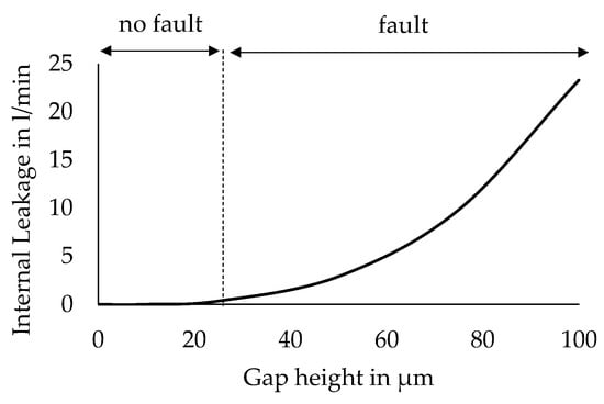
Figure 4.
Example of non-uniform class distribution over the range of fault-indicating parameters.
For the application of methods of supervised learning, the generated data instances must be provided along with their class labels, which, in the framework of condition monitoring, indicate the fault state of the considered system. Here, the labels are defined for the single-target classification of binary classes. In the process of simulative data generation, continuous model parameters are used to indicate and adjust the fault intensities. Now, these fault-indicating parameters are transformed into categorical class labels by binning parameter ranges to classes of “fault” and “no fault”. The threshold values, which define whether a certain degradation level is considered a fault or not, depend on the specific application and the tolerances allowed therein. In this study, the threshold values listed in Table 1 are used. For the three different leakage faults, thresholds are set under consideration of the leakage flows resulting at the respective fault intensities. The defined thresholds of the gap heights, which mark the beginning of a fault for the internal and external leakage at the cylinder, produce volumetric leakage flows of 0.36 L/min and 0.1 L/min, respectively, at 40 °C and a differential pressure of 150 bar. The threshold value for the leakage factor, which marks the beginning of a fault of external leakage at the hydraulic power supply, is equivalent to a leakage flow of 0.1 L/min at 40 °C and the maximal pressure of 200 bar. For the other three faults, the thresholds are determined heuristically.
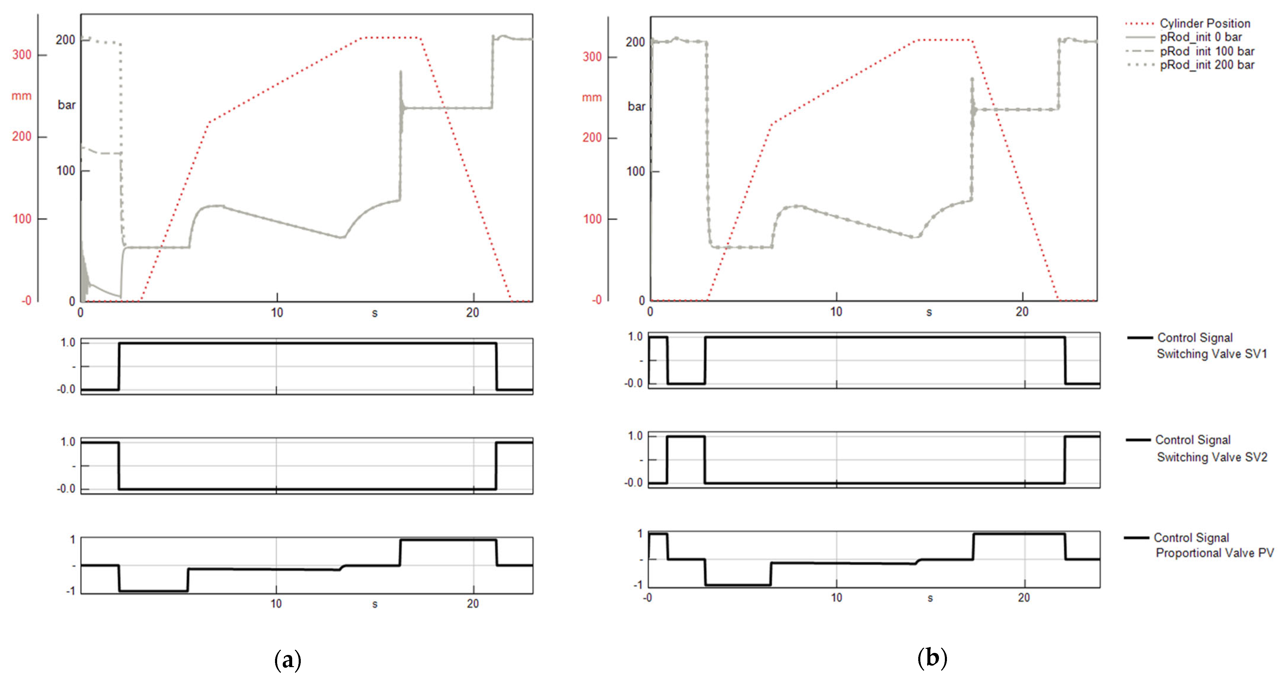
Another issue that arises during the variational study is the setting of the initial conditions for the simulation runs. Because model parameters are constantly varied between simulation runs, a single initial system condition, which is valid for all runs, cannot be determined. In order to circumvent this issue, the simulated press cycle is considered to represent one cycle within a series of multiple press cycles. As a result, the initial state of the system is determined by the state at the end of the previous cycle. To achieve this, every simulation run is started with the final second of the control sequence of the working cycle, instead of only simulating the actual working cycle. Afterwards, the first second of the simulated cycle is removed after the data are generated. Consequently, setting the initial conditions of the simulation is no longer critical while performing the variational study. The described approach and its effects are shown in Figure 5 by the example of the pressure at the rod side of the hydraulic cylinder. When only simulating the actual working cycle, the progression of the rod-side pressure depends on the selection of the initial value, as Figure 5a shows. In contrast, Figure 5b shows that starting the simulation run with the ending sequence of a cycle allows to obtain results independent of the selected initial condition, when the first simulated second is removed afterwards.
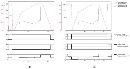
Figure 5.
Cylinder position, cylinder pressures and valve control signals simulated under fixed initial conditions while (a) starting the simulation with the actual control sequence of the press cycle and (b) starting the simulation with the ending sequence of a press cycle prior to the actual control sequence.
3.3. Feature Extraction and Selection
Before using the generated data for training a fault classification model, the raw time series are transformed into a fixed number of features. For this, the python-based open-source package tsfresh is used, which provides the calculation of a large variety of features for time series [23]. As the features must be calculated for each of the eight subsignals of the 200,000 multivariate time series, the following base set of 16 features with low computational costs is extracted:
- minimum;
- maximum;
- mean;
- median;
- standard deviation;
- variance;
- skewness;
- kurtosis;
- first location of minimum;
- first location of maximum;
- last location of minimum;
- last location of maximum;
- sum of values;
- absolute energy (sum over squared values);
- absolute sum of changes (sum over absolute values of consecutive changes);
- mean absolute change (mean over absolute values of consecutive changes).
Extracting this base set of features for a time series yields a feature vector of 128 features for one data instance. Generally, the resulting feature vectors only comprise subsignals recorded during data generation. However, derivations and transformations of the raw data often can reveal additional information about the characteristics of a signal. Moreover, the extracted features only represent characteristics over complete working cycles and thus only carry information on the aggregated effect of a fault on the observed data. In contrast, a conventional, visual inspection of sensor data by a human expert would typically involve a detailed inspection of anomalies in specific segments of the working cycle, such as checking for leakages in idle mode or the maximal cylinder velocity in rapid traverse. Such short-term effects can even be attenuated, when computing features over complete working cycles. Consequently, in this study, the state-of-the-art feature extraction is extended by incorporating further information into the feature extraction, which is typically available or can be acquired easily.
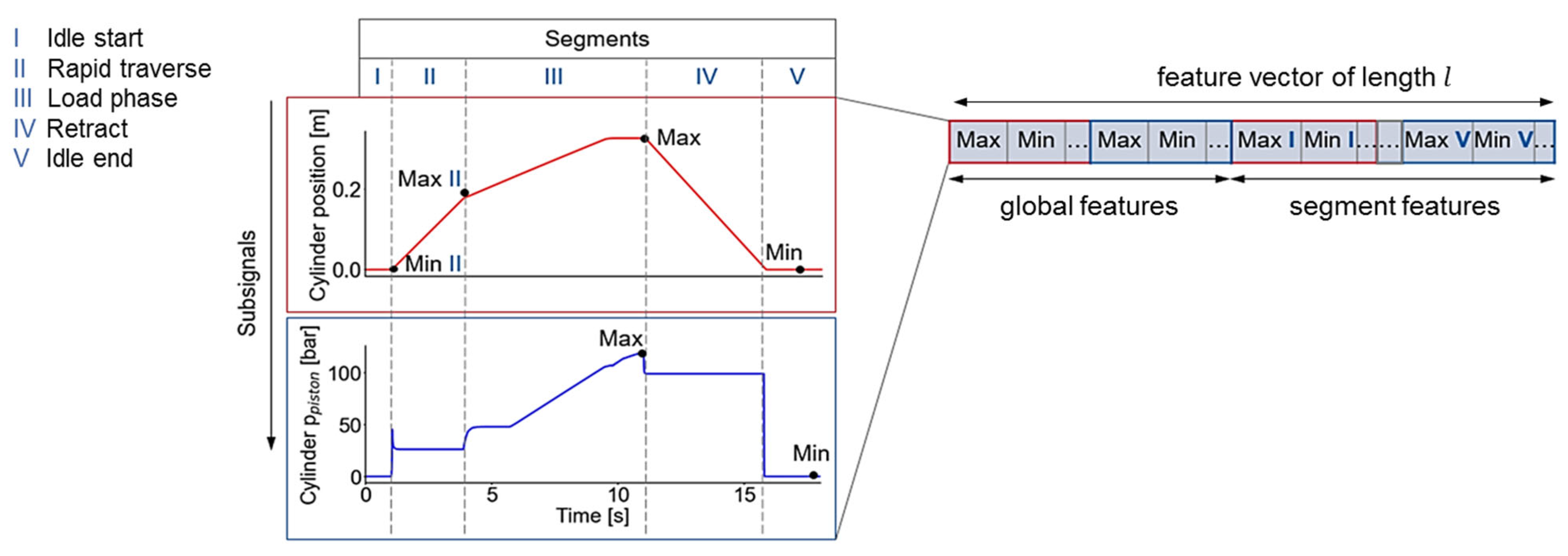
The first step of the extension consists in adding information about the progression of the recorded subsignals over time. This information is obtained by computing the first time derivatives of the subsignals and adding them to the time series as further subsignals. As a result, the number of subsignals is doubled and the number of extracted features per time series increases accordingly. The second step of the extension focusses on accentuating the characteristics of the subsignals in specific segments of the working cycle. For this, each time series is divided into segments of constant operation phases. These are the idle phases at the beginning and end of the cycle, rapid traverse, load phase and the backstroke. The transitions between operation phases are inferred from control signals given by the machine control. Subsequently, the same set of features that is extracted for the complete time series is again extracted for each subsignal in each of the defined segments, as Figure 6 illustrates for the features “maximum” and “minimum”. In the framework of this contribution, the originally generated feature set is referred to as global features, while the newly added features are referred to as segment features. The length l of the feature vector that represents a single data instance is again increased and now given by Equation (1), where , and denote the number of subsignals, features and segments, respectively. Altogether, extracting features from the full time series and its five segments results in a set of 1536 features.
l = nsubsignals ∙ nfeatures ∙ (1 + nsegments)
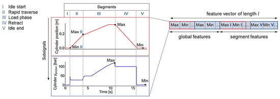
Figure 6.
Concept of adding segment features to the base set of global features shown for two subsignals and the features “maximum” and “minimum”.
As a result of the extended feature extraction, the number of features is increased, with the aim to also increase the amount of extracted information. However, not all the additionally generated characteristics can be assumed to be useful for fault classification. Concurrently, a concise set of features without irrelevant and redundant information is preferable for the efficient and robust training of most machine learning models and algorithms [19]. Moreover, a small set of only relevant features enables a human inspection and comprehension of the information fed to a classification model and consequently leads to higher transparency of the inference process. Therefore, feature selection follows, to reduce the set of features to those useful for the respective fault classification. This is achieved by using a wrapper method with decision tree classifiers. This means that a classification model is trained with the primary purpose of accessing the features implicitly selected within the model.
A decision tree classifier is a machine learning model that aims at hierarchically dividing a given dataset into groups of homogenous classes [27], which, in this case, are the classes “fault” and “no fault”. The decision rules derived during training are based on defining threshold values for certain features, which then allow to classify a data instance. After training, the features and the corresponding threshold values of the different decision nodes can be inspected. Subsequently, it can be comprehended which features enable the effective separation of the data instances. Figure 7 shows the first two levels of a decision tree for the classification of internal cylinder leakage. Moreover, decision trees, and their underlying algorithm, show low sensitivity of classification performance to the size of the feature sets that they are trained with [19], which makes them well suited for the task of processing the initially large feature set. To mitigate the tendency of decision trees to overfit, the maximum number of levels of the trees is limited. A maximum of five levels is heuristically found to provide a low variance of classification accuracy with no indication of overfitting.
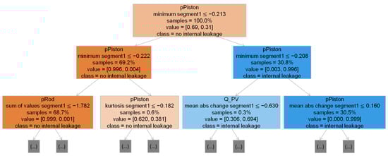
Figure 7.
First two levels of a decision tree for the classification of internal leakage at the cylinder. Threshold values relate to features scaled by means of standardization.
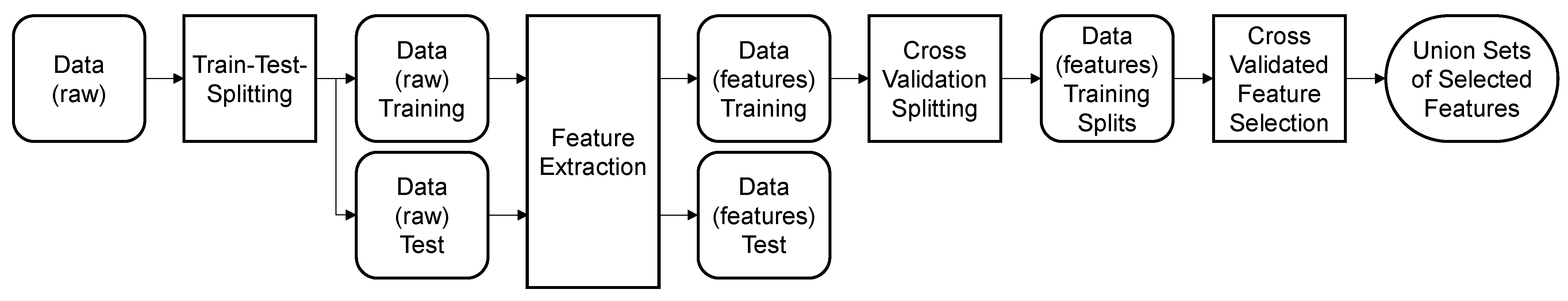
As each of the considered component faults of the hydraulic press has a different impact on the machine behavior, the feature selection procedure is repeated for each of the considered faults. Furthermore, the resulting sets of selected features can depend on the specific set of training data used during selection. Random elements included in the CART algorithm, which is here used for training the decision trees, further add to the stochastic variation of the training results. Therefore, the feature selection is performed in the form of a 5-fold cross-validation. For this, the training and testing of each decision tree is repeated five times, using different excerpts of the data for training and testing in each repetition. Finally, the union set of features selected in all repetitions is formed and used for the training the final classification models. Figure 8 shows the procedure of feature extraction and cross-validated feature selection. The data scaling is not illustrated therein, but standardization is performed within the cross-validation for each training and testing split individually.
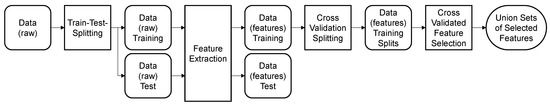
Figure 8.
Process of feature extraction and cross-validated feature selection.
3.4. Model Setup, Training and Evaluation
Apart from the decision tree classifiers used during feature selection, the final fault classification is realized using feedforward neural networks. The problem of classifying the machine state is set up as a composition of single-target classifications with binary targets. This means that a model for binary classification is set up and trained for each of the considered component faults individually. This allows us to build smaller models, which potentially can be trained more efficiently and transparently. Moreover, modular fault classification models can be generated independently and on demand, while multi-target classification would require the a priori definition of all possible fault cases that can be expected in a system. Furthermore, using a separate classifier for each fault allows to obtain a diagnosis without the issue of an exponential increase in the number of class labels with an increasing number of faults, as would be the case in multi-target, multi-class classification. However, one disadvantage of the considered setup is that interdependencies between fault occurrences cannot be considered by the models.
The hyperparameters of the feedforward neural networks comprise the structural hyperparameters of the network, such as the number of hidden layers, number of nodes per layer and activation function of each layer, as well as fitting hyperparameters such as the loss function and the learning rate. As with the definition of the labels described previously in this section, the definition of the fitting hyperparameters depends on the definition of the problem at hand. Given that a binary classification is the targeted task, options for selecting the loss function are narrowed down to loss metrics, which are suitable for evaluating the outputs of the model against binary labels. Here, the binary cross-entropy is used as a loss metric. Furthermore, the selection of a learning rate can be simplified to only defining a starting learning rate when a state-of-the-art optimization algorithm with an adaptive learning rate is used. The Adam algorithm is used in this study, with a default setting of the starting leaning rate of 0.001.
Similarly, the numbers of nodes on the input layers and output layers of the neural networks are predetermined by the number of features fed to the models and the number of labels to predict, respectively. While the input layer is set to have a ReLU activation function, a sigmoid activation function is used in all hidden layers and the output layer. Further structural hyperparameters of the neural networks, which are the number of hidden layers and the number of nodes therein, are determined by means of a grid search. Different model structures are set up and trained so that the best model structure of the considered configurations can be identified for each fault case. The scheme of the grid search and the concept of varying the model structure are shown in Figure 9. The scheme shows that three different numbers of hidden layers and four different settings of the maximal number of nodes are varied. For a given number of hidden layers, the first hidden layer is constructed with the maximal number of nodes defined. Then, in each subsequent layer, the number of nodes is halved.
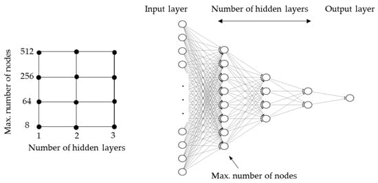
Figure 9.
Applied scheme of grid search and corresponding model hyperparameters.
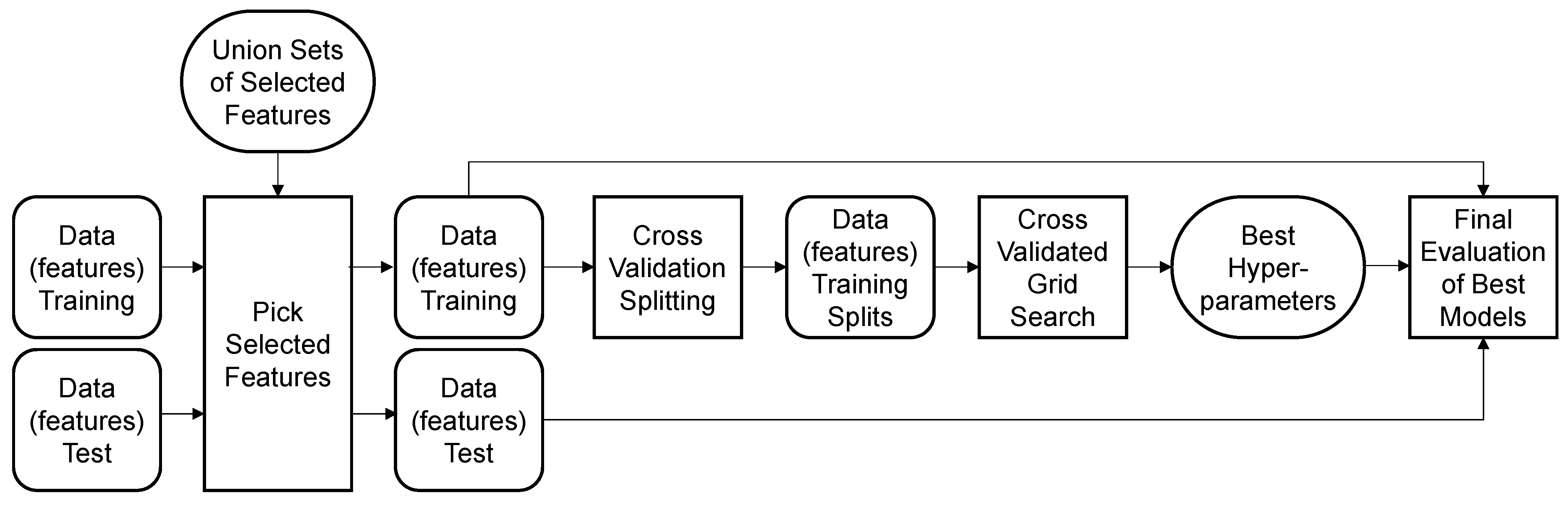
As with the feature selection step, each model configuration considered in the grid search is trained and tested with different excerpts of the data within a 5-fold cross-validation. A further test set, which is held out from the whole process of feature selection and model tuning, is finally used to evaluate the performance of the models selected in the grid search. The test set comprises around 40,000 working cycles, which is 20% of the available data. This form of validation procedure is referred to as the three-way holdout method and is required to obtain an unbiased, final estimate of the model performance, as the test data used in the cross-validation loop were already involved during feature selection and grid search [28]. The classification performance of the models is evaluated using the balanced accuracy. The balanced accuracy is defined as the mean value of the true-positive rate and the true-negative rate and thus gives a balanced estimate independent of the class distribution of the data [29]. The applied procedure of the cross-validated grid search is illustrated in Figure 10.
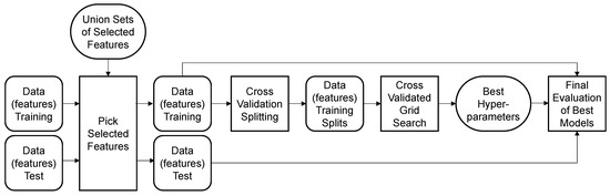
Figure 10.
Procedure of cross-validated grid search and final evaluation of models following the three-way hold-out method.
4. Results
4.1. Results of the Grid Search
The mean classification accuracies of the best models identified in the grid search are shown in Table 2 for the different faults, for different feature sets, as well as with and without feature selection. Table 3 lists the corresponding structures of these models. For the faults of internal cylinder leakage , the position sensor offset and the external leakage at the hydraulic power supply , high classification accuracies around 99% are already obtained with the base set of global features. This range of accuracies is obtained for these faults with all tested structural configurations of the neural networks, with no clear dependence on model size and a maximal deviation between the best- and worst-performing models of less than 1% across all feature sets. Therefore, the smallest possible model structure (one hidden layer with eight nodes) is also considered the best-performing model for these faults. A marginal increase in the model performance can be observed for these three faults when extending the feature sets and applying feature selection. For the fault of worn control edges on the proportional valve , a similar trend is observed when increasing the feature set, while the feature selection does not always lead to improved maximal performance. Regarding the model size, however, the feature selection leads to the same effect as stated above for other faults, where the difference in performance between model sizes becomes marginal and the smallest models can be regarded as the best-performing models for a specific configuration. Using an increased set of features clearly improves the performance of the classifiers for the faults of increased friction at the cylinder and an external leakage at the cylinder . The prediction of increased friction appears to benefit from added derivative and segment features likewise. In contrast, for the external leakage, the information added by segment features appears to mainly induce the improvement, especially when no feature selection is applied. Moreover, for both latter faults, the best-performing models have larger network structures when feature selection is considered. While the achieved maximal accuracies can be considered high performance scores for the increased friction and the external cylinder leakage, the models cannot fully resolve the targeted input–output relationship with the given data and considered model structures.
Table 2.
Mean classification accuracies obtained with the best model during the grid search with and without feature selection, for different feature sets and for different faults. Best results for each fault are highlighted in bold.
Table 3.
Structure of the hidden layers of the best models obtained from the grid search with and without feature selection, for different feature sets and for different faults.
A final evaluation of the classification performance of the identified model structures is performed on a held-out test set, which was not involved during the cross-validated feature selection and grid search. This is carried out to validate that the trained models are not overfitted to the training data and that the features selected during feature selection are also important for classifying new, unseen data instances. For this, all the data, which were partitioned into five subsets during cross-validation, are jointly used to train the models that were identified as the best model structures during the grid search. The results are given in Table 4 and show that, generally, the same scores are achieved as given in Table 2 and estimated during the cross-validated grid search. Moreover, the scores obtained on the test set are mostly slightly higher, which can be attributed to the larger set of training data used in this final evaluation.
Table 4.
Classification accuracies obtained with the best model structure on the held-out test set with and without feature selection, for different feature sets and for different faults. Best results for each fault are highlighted in bold.
4.2. Results of the Feature Selection
Apart from the effects discussed in the previous subsection, further effects of the feature selection are described in the following. Table 5 shows the number of features selected from the different feature sets for the different faults. Compared to the case of no feature selection, the number of features is significantly reduced after selection in all the listed cases. Moreover, considering the number of selected features across feature sets, for most faults, the number of selected features steadily increases when increasing the feature set before selection. The main increase in the number of selected features compared to the base set of global features is obtained by adding segment features, which is in alignment with the increase in performance induced by the segment features observed in the previous subsection. The exception is the fault of increased friction , where a higher number of features is selected that represent trend information of the time series.
Table 5.
Number of features before and after feature selection for the different feature sets and different faults.
A benefit of a reduced set of features is that it enables to inspect features manually. This allows us to gain an insight into the process of fault inference and into the general system behavior under faults. Moreover, using decision trees for feature selection, the selected features are provided with relative importance, which indicates which fraction of the data instances could be separated into classes of “fault” and “no fault” by using this feature. Accordingly, a ranking of the features is obtained, in addition to the reduction. However, as the feature selection is performed in a cross-validation loop and union sets of selected features are formed afterwards, the ranking information is not maintained after this step. Therefore, the ranking information is acquired from a single run of the cross-validation loop. In Table 6, the three most important features selected for each of the considered faults are listed. The subsignals can be found in the hydraulic circuit diagram in Figure 2.
Table 6.
Three most important features identified through feature selection for each fault.
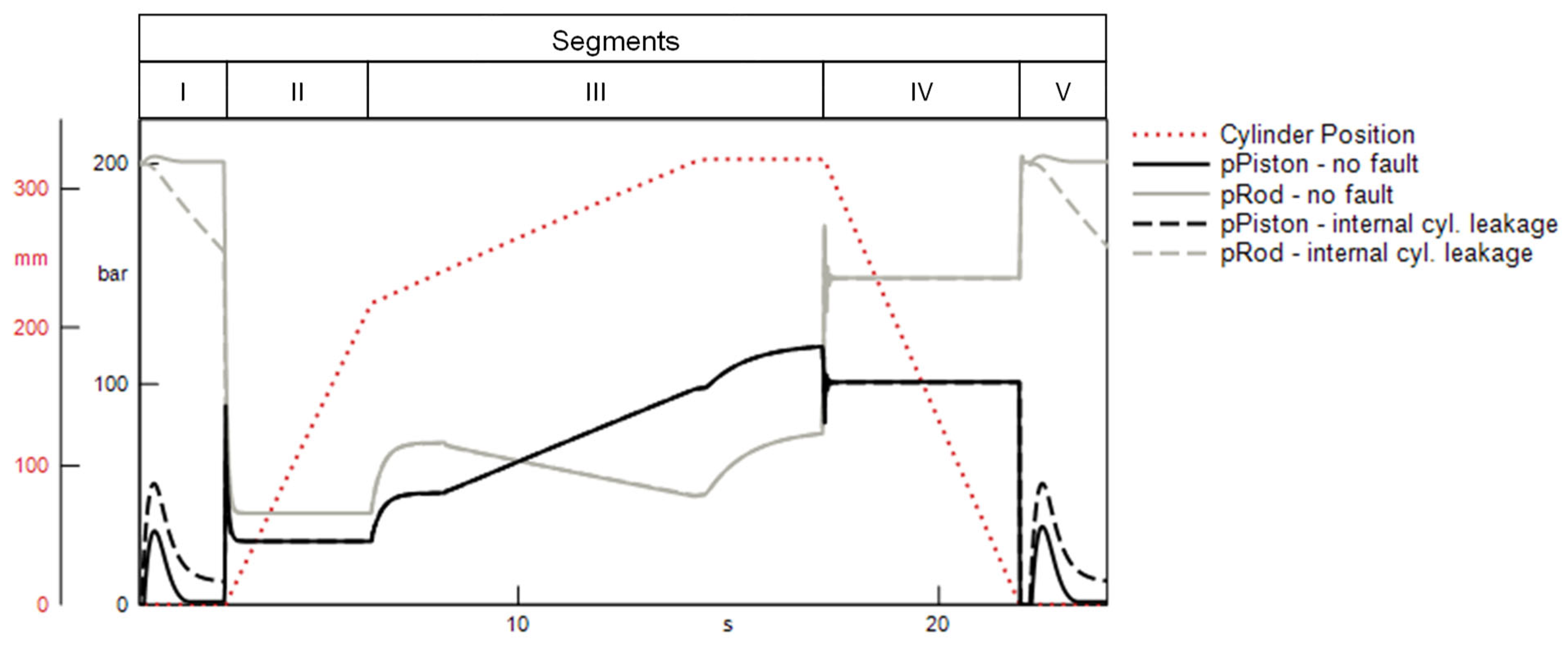
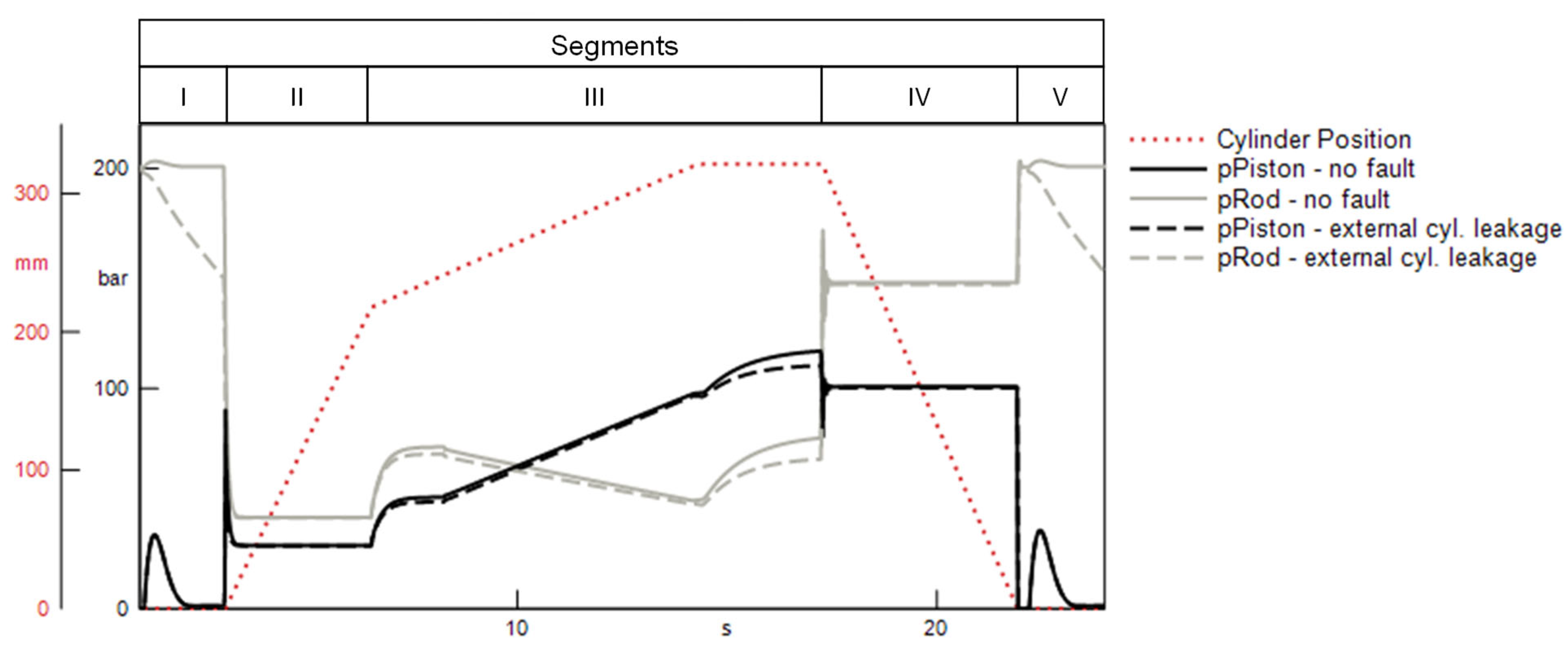
To check the plausibility of the selected features, an exemplary visual inspection of the respective subsignals is performed. Figure 11 shows the progression of the pressures recorded at the hydraulic cylinder in regular operation, as well as under the influence of an internal cylinder leakage . For the detection of this fault, the minimum of the pressure on the piston side of the cylinder in the idle phase at the beginning of the press cycle (segment I) is selected as the most important feature. This is in accordance with the observed subsignals shown in Figure 11. An internal leakage clearly alters the pressure progression in the idle phases at the beginning and end of the press cycle. Moreover, an internal leakage leads to an increased pressure level at the piston side and thus to an altered minimum value of this pressure. This increase is induced by the pressure equalization between the two cylinder chambers, which is enabled by the existence of a leakage gap. An example for the effect of an external cylinder leakage on both cylinder pressures is shown in Figure 12. For this fault, the minimum value of the pressure on the piston side during the load phase (segment III) is selected as the most important feature. Again, the selection of this feature appears plausible, as this characteristic of the rod-side pressure is uniquely impacted by the occurrence of the external leakage. Additionally, the drop in the rod-side pressure in segments I and V is strongly affected by the external leakage. However, the fact that this symptom is also observed with an internal cylinder leakage explains why this feature was not selected as important indicator of an external cylinder leakage.
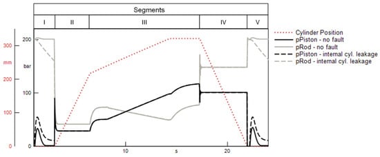
Figure 11.
Simulated effect of an internal cylinder leakage on the cylinder pressures.
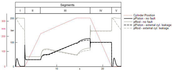
Figure 12.
Simulated effect of an external cylinder leakage on the cylinder pressures.
5. Discussion
Overall, the results show that the generic development procedure applied in this study allows to effectively develop fault classification models for the condition monitoring of a hydraulic press. In general, the results show that different faults in the system require different model structures and information for their effective classification. Especially for the faults of the internal leakage at the cylinder, the offset at the position sensor and the external leakage at the hydraulic power supply could be inferred with a base set of generic features and small neural network structures. This indicates that the occurrence of these faults uniquely impacts a small set of features, independently of other faults and operating conditions. For the other faults, the presented approach of extended feature extraction was shown to clearly impact the performance of the respective classification models. The difference in required features and obtained model sizes indicates the sensibility of the applied approach in performing single-target classifications for each fault individually, instead of defining a multi-target task to predict all faults concurrently.
In contrast to extending the feature set, the feature selection does not clearly affect the maximal model performance, regardless of the feature set and fault considered. The feature selection, however, impacts the sizes of the model structures of the best-performing models. Except for the fault cases, where the smallest considered model structure was sufficient, the best-performing models had larger network structures when feature selection was applied. The results indicate that the feature selection yields larger models, when the relationship between features and the existence of a fault cannot be fully resolved. This is particularly indicated by the results for the fault of worn control edges of the proportional valve, shown in Table 2 and Table 3. As the feature set is increased and the classification accuracy approaches a level of 99%, the difference in performance between different model structures diminishes and smaller models achieve the same performance as larger model structures. Another aspect to consider is that, in the grid search, only the structure of hidden layers was varied, while the number of input layers depended on the size of the feature vector fed to the model. Consequently, a larger set of features at the input also adds a larger number of model parameters to start with.
Finally, the feature selection provides an insight into the development workflow and increases the transparency of the data-driven development. This is especially the case when human-interpretable features are extracted from the raw time series data. For the examples of an internal and external cylinder leakage, it was shown that the feature selection provided plausible information on symptoms uniquely caused by certain faults.
Author Contributions
Conceptualization, F.M. and K.S.; methodology, F.M.; software, F.M.; validation, F.M.; investigation, F.M.; data curation, F.M.; writing—original draft preparation, F.M.; writing—review and editing, K.S. and F.M.; supervision, K.S.; project administration, F.M. and K.S.; funding acquisition, K.S. All authors have read and agreed to the published version of the manuscript.
Funding
The authors thank the Research Association for Fluid Power of the German Engineering Federation VDMA for its financial support. Special gratitude is expressed to the participating companies and their representatives in the accompanying industrial committee for their advisory and technical support.
Institutional Review Board Statement
Not applicable.
Informed Consent Statement
Not applicable.
Data Availability Statement
The datasets generated during and/or analyzed during the current study are available from the corresponding author on reasonable request.
Conflicts of Interest
The authors declare no conflict of interest.
References
- ISO 17359:2018; Condition Monitoring and Diagnostics of Machines—General Guidelines (ISO 17359:2018). International Organization for Standardization: Geneva, Switzerland, 2018.
- Watton, J. Modelling, Monitoring and Diagnostic Techniques for Fluid Power Systems; Springer: London, UK, 2007; ISBN 9781846283734. [Google Scholar]
- Isermann, R. Fault-Diagnosis Systems; Springer: Berlin/Heidelberg, Germany, 2006; ISBN 978-3-540-24112-6. [Google Scholar]
- Alt, R.; Murrenhoff, H.; Schmitz, K. A Survey of “Industrie 4.0” in the Field of Fluid Power—Challenges and Opportunities by the Example of Field Device Integration. In Proceedings of the 11th International Fluid Power Conference, Aachen, Germany, 19–21 March 2018; Murrenhoff, H., Ed.; RWTH Aachen University: Aachen, Germany, 2018. ISBN 3958862152. [Google Scholar]
- Kuhn, M.; Johnson, K. Applied Predictive Modeling, Corrected at 5th Printing; Springer: New York, NY, USA, 2016; ISBN 978-1-4614-6848-6. [Google Scholar]
- Döbel, I.; Leis, M.; Vogelsang, M.M.; Neustroev, D.; Petzka, H.; Rüping, S.; Voss, A.; Wegele, M.; Welz, J. Maschinelles Lernen—Kompetenzen, Anwendungen und Forschungsbedarf: Projektbericht. 2018. Available online: https://www.bigdata-ai.fraunhofer.de/content/dam/bigdata/de/documents/Publikationen/BMBF_Fraunhofer_ML-Ergebnisbericht_Gesamt.pdf (accessed on 28 July 2022).
- Paulmann, G.; Mkadara, G. Condition monitoring of hydraulic pumps—Lessons learnt. In Proceedings of the 11th International Fluid Power Conference, Aachen, Germany, 19–21 March 2018; Murrenhoff, H., Ed.; RWTH Aachen University: Aachen, Germany, 2018. ISBN 3958862152. [Google Scholar]
- Torikka, T.; Haack, S. Predictive Maintenance Service Powered by Machine Learning and Big Data. In Proceedings of the 11th International Fluid Power Conference, Aachen, Germany, 19–21 March 2018; Murrenhoff, H., Ed.; RWTH Aachen University: Aachen, Germany, 2018. ISBN 3958862152. [Google Scholar]
- Schraft, J.P.; Becher, D.; Weber, J. Condition Monitoring Strategy for Pump-Driven Hydraulic Axes. In Proceedings of the ASME/BATH Symposium on Fluid Power and Motion Control, Online, 9–11 September 2020; The American Society of Mechanical Engineers: New York, NY, USA, 2020. ISBN 9780791883754. [Google Scholar]
- Azeez, A.A.; Vuorinen, E.; Minav, T.; Casoli, P. AI-based condition monitoring of a variable displacement axial piston pump. In Proceedings of the 13th International Fluid Power Conference, Aachen, Germany, 13–15 June 2022; Schmitz, K., Ed.; RWTH Aachen University: Aachen, Germany, 2022. [Google Scholar]
- Wiens, T.; Fernandes, J. Application of Data Reduction Techniques to Dynamic Condition Monitoring of an Axial Piston Pump. In Proceedings of the ASME/BATH Symposium on Fluid Power and Motion Control, Longboat Key, FL, USA, 7–9 October 2019; The American Society of Mechanical Engineers: New York, NY, USA, 2020. ISBN 9780791859339. [Google Scholar]
- Yao, J.; Li, X.; Wang, P.; Cheng, Y.; Yang, S. Data-driven Fault Diagnosis Based on Deep Learning for Multiple Failures of High Speed On/off Valve. In Proceedings of the 13th International Fluid Power Conference, Aachen, Germany, 13–15 June 2022; Schmitz, K., Ed.; RWTH Aachen University: Aachen, Germany, 2022. [Google Scholar]
- Ali, E. Self-Learning Condition Monitoring for Smart Electrohydraulic Drives. Ph.D. Thesis, Technische Universität Dresden, Dresden, Germany, 2019. [Google Scholar]
- Torikka, T. Bewertung von Analyseverfahren zur Zustandsüberwachung einer Axialkolbenpumpe. Ph.D. Thesis, Shaker, Aachen, Germany, 2011. [Google Scholar]
- Duensing, Y.; Rodas Rivas, A.; Schmitz, K. Machine Learning for Failure Mode Detection in Mobile Machinery. In Proceedings of the 11th Kolloquium Mobilhydraulik, Karlsruhe, Germany, 10 September 2020; Geimer, M., Synek, P.-M., Eds.; KIT Scientific Publishing: Karlsruhe, Germany, 2020; pp. 1–25. [Google Scholar]
- Helwig, N.J. Zustandsbewertung Industrieller Prozesse Mittels Multivariater Sensordatenanalyse am Beispiel Hydraulischer und Elektromechanischer Antriebssysteme. Ph.D. Thesis, Shaker, Aachen, Germany, 2019. [Google Scholar]
- Adams, S.; Beling, P.; Farinholt, K.; Brown, N.; Polter, S.; Dong, Q. Condition Based Monitoring for a Hydraulic Actuator. In Proceedings of the Annual Conference of the PHM Society, Bilbao, Spain, 5–8 July 2016. [Google Scholar]
- Makansi, F.; Schmitz, K. Feature Generation and Evaluation for Data-Based Condition Monitoring of a Hydraulic Press. In Proceedings of the 13th International Fluid Power Conference, Aachen, Germany, 13–15 June 2022; Schmitz, K., Ed.; RWTH Aachen University: Aachen, Germany, 2022. [Google Scholar]
- Kuhn, M.; Johnson, K. Feature Engineering and Selection: A Practical Approach for Predictive Models; Chapman & Hall/CRC: Boca Raton, FL, USA, 2021; ISBN 978-1-03-209085-6. [Google Scholar]
- Aggarwal, C.C. Neural Networks and Deep Learning: A Textbook; Springer International Publishing: Cham, Switzerland, 2018; ISBN 978 3 319 94462 3. [Google Scholar]
- Hornik, K.; Stinchcombe, M.; White, H. Multilayer feedforward networks are universal approximators. Neural Netw. 1989, 2, 359–366. [Google Scholar] [CrossRef]
- Géron, A. Hands-on Machine Learning with Scikit-Learn, Keras, and TensorFlow; O’Reilly Media, Inc.: Sebastopol, CA, USA, 2019. [Google Scholar]
- Christ, M.; Kempa-Liehr, A.W.; Feindt, M. Distributed and Parallel Time Series Feature Extraction for Industrial Big Data Applications. 2016. Available online: http://arxiv.org/pdf/1610.07717v3 (accessed on 28 July 2022).
- Radford, A.; Metz, L.; Chintala, S. Unsupervised Representation Learning with Deep Convolutional Generative Adversarial Networks. 2015. Available online: http://arxiv.org/pdf/1511.06434v2 (accessed on 28 July 2022).
- ESI Group. SimulationX. Available online: https://www.esi-group.com/products/system-simulation (accessed on 28 July 2022).
- Makansi, F.; Schmitz, K. Simulation-Based Data Sampling for Condition Monitoring of Fluid Power Drives. IOP Conf. Ser. Mater. Sci. Eng. 2021, 1097, 012018. [Google Scholar] [CrossRef]
- Fürnkranz, J. Decision Tree. In Encyclopedia of Machine Learning and Data Mining; Sammut, C., Webb, G.I., Eds.; Springer: Boston, MA, USA, 2017; pp. 330–335. ISBN 978-1-4899-7685-7. [Google Scholar]
- Raschka, S. Model Evaluation, Model Selection, and Algorithm Selection in Machine Learning. 2018. Available online: http://arxiv.org/pdf/1811.12808v3 (accessed on 28 July 2022).
- Brodersen, K.H.; Ong, C.S.; Stephan, K.E.; Buhmann, J.M. The Balanced Accuracy and Its Posterior Distribution. In Proceedings of the 2010 20th International Conference on Pattern Recognition (ICPR), Istanbul, Turkey, 23–26 August 2010; IEEE: Piscataway, NJ, USA, 2010; pp. 3121–3124, ISBN 978-1-4244-7542-1. [Google Scholar]


Publisher’s Note: MDPI stays neutral with regard to jurisdictional claims in published maps and institutional affiliations. |
© 2022 by the authors. Licensee MDPI, Basel, Switzerland. This article is an open access article distributed under the terms and conditions of the Creative Commons Attribution (CC BY) license (https://creativecommons.org/licenses/by/4.0/).