Abstract
The operation of the photovoltaic (PV) system under partial shading conditions (PSC) is complicated since the output characteristic of the PV system is profoundly affected by the heterogeneous irradiance of PSC. This paper proposes a dynamic reconfiguration framework to tackle PSC in the PV array. Continuous operation of the dynamic PV array reconfiguration under cloud-induced partial shading is considered by developing an emulator of the moving cloud. In addition, the Particle Swarm Optimization and Rao algorithms are improved to obtain the optimal PV array configuration under PSC. The operation of switching is enhanced by simultaneously considering the total switching times and the operation of highly active switches. The simulation results on the PV array demonstrate the effectiveness of the proposed framework in terms of reducing the number of local maximum power points on the power-voltage characteristic, enhancing power output, and relieving stress on the switching operation of the PV array under different PSC.
1. Introduction
Partial shading conditions (PSC) commonly occur on PV arrays. Such phenomena could cause detrimental effects on the PV array: reducing PV output power, misleading the function of the maximum power point (MPP) tracker by introducing multiple local MPPs on the power-voltage curve of the PV array, and creating hot spots on the PV panels. To minimize the effects of PSC on the PV array, multiple studies [1,2,3,4,5,6,7,8,9,10,11,12] have been conducted, in which studies on PV array reconfiguration (PVAR) have been considered promising solutions. The PVAR involves changing electrical connections between PV modules in the PV array either by rewiring connections or by switching at terminals of connections of the PV array. Studies [4,5,6,7] disperse the shadow by rewiring connections of the PV modules of the PV array. The rewiring process happens one time, then the configuration is fixed under operation. Thus, these models are called static PVAR. Although this approach does not require any moving mechanisms during the operation, the rewiring process is complicated, especially for large PV systems. In addition, as the configuration of the PV array is fixed in operating conditions, the effectiveness of the reconfigured PV array is limited under certain PSC. On the other hand, [8,9,10,11,12] distribute the shadow in the PV system by continuously switching the terminal connections of PV modules, which is called dynamic PAR (DPVAR). Compared to static PVAR models, DPVAR models are more adaptive under different PSC [6]. Although many studies on DPVAR have been proposed, many of these models do not consider the variability of cloud-induced shade, which is a typical shade happening in reality.
Studies [4,6,13] have modeled the shading patterns based on the width, length, and position of the shade. However, the fidelity of such shading emulations is limited as they only cover some certain ideal and fixed shading patterns. In reality, the moving shade frequently changes its properties, such as shape, size, direction, speed, and thickness, during the time passing on the PV array. In addition, the transition between shading situations has not been properly addressed. Recent studies modeled the variability of the shade by folding many shading situations altogether. However, the time resolution between each transition is still high: hourly in [11,14,15] models and minutely in [16] model. Moreover, the thickness and the shape of the shade are assumed to remain unchanged during the shade passing on the PV array. The effect of the execution time of the DPVAR on the performance of the reconfiguration has not been evaluated. As a result, these models have not fully proven their abilities in dealing with variable shades and the link between transitions is not clearly stated.
One crucial step in creating an effective DPVAR framework is developing the reconfiguration algorithm (RA) [8]. Ref. [8] utilizes bubble-sort and model-based methods to determine optimal configuration by combining the adaptive part and the fixed part of the PV array. In [10], Dynamic Programming is used to obtain the optimal configuration. Subsequently, [11] proposes an improved Dynamic Programming to enhance the capability of the searching algorithm. Recently, heuristic-based RAs have become prevalent: genetic algorithm [17], particle swarm optimization algorithm (PSO) [18], grasshopper optimization algorithm [19], flow regime algorithm [14], the social mimic optimization algorithm [14], the Rao optimization algorithm [14], and butterfly optimization algorithm [20]. These models are suitable for real-life systems, where the shading patterns and PV characteristics are diverse. Although many heuristic algorithms have been applied to the DPVAR problem, these models lack DPVAR-problem-specific features in their algorithms.
Another challenge of the DPVAR involves designing the complicated switching board. Ref. [9] proposes a switching matrix for the Electrical Array Reconfiguration generator topology. However, this design is only applicable to small systems [21] develops Dynamic Electrical Scheme (DES), which is more adaptive to different system scales. However, the DES attains its high flexibility at the expense of utilizing a large number of switches and requiring many switching times. Previous DPVAR models only consider switching operation as a by-product of the power-optimized configuration.
As can be acknowledged from the above literature reviews, there are several knowledge gaps in DPVAR that have not been addressed:
- DPVAR models have not considered sufficiently the variability of the shade. Moreover, the link of solutions over time and the influence of the execution time of the DPVAR are not mentioned.
- Shading emulators lack practical properties: shape, size, direction, speed, and thickness.
- RA still can be improved by specifically designed for the DPVAR problem.
- Switching operation has not been directly optimized.
In this study, a new framework for the DPVAR problem is proposed. The proposed framework is validated on the frequently-used TCT configuration in continuous operation under moving clouds (MC), which is the most common type of variable shade. The contributions of this paper are briefly folded as follows:
- Evaluate continuous PSC on the DPVAR by accessing properties of MC: shape, size, thickness, and position (related to speed and direction).
- State the PSO and Rao algorithms for the DPVAR problem, and propose three techniques to improve the performance of the RA: diversifying population, updating velocity during the optimization process, and screening low-quality solutions.
- Evaluate the effects of the transition between shading situations and the execution time of the DPVAR on the overall performance of the DPVAR.
- Optimize the operation of switching: reduce total switching times and reduce the number of switching on the active switches.
The efficacy of the model is validated in two operation modes, including single-time step operation and continuous time step operation.
2. Model Descriptions
2.1. PV Modeling
In the PVAR problem, a PV unit is usually modeled to the module scale to strike the balance between the computational cost and the modeling accuracy [14,22]. In this study, the single-diode model, which is frequently used in PV modeling [23,24,25,26], is employed to simulate the output characteristics of the PV module under PSC. The single-diode model is presented by an equivalent circuit in Figure 1a.
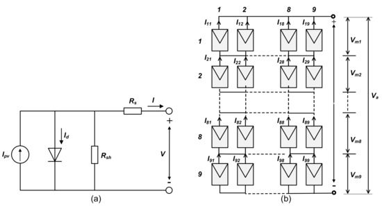
Figure 1.
(a) Equivalent circuit of single-diode PV model. (b) TCT configuration of PV array.
In this model, [A] is the photo-generated current; [A] is the dark diode current; [A] is the reverse saturation current [A]; a is the diode’s ideal factor; and are the series resistor and shunt resistor, respectively. The output current-voltage of this electrical circuit is expressed by (1).
where is the number of cells in a PV module, k is the Boltzmann constant, and q is the electron charge. The I-V characteristic of a PV module is identified by estimating five parameters (, , a, , ) in (1). The detailed process of identifying the I-V characteristic of the PV module is presented in our last studies [23,24].
To meet the required power output of practical applications, PV modules are connected together to form the PV array. In this study, the DPVAR problem is considered on the most frequently-used PV array configuration, total-cross-tied (TCT), which is depicted in Figure 1b. The output voltage of the studied PV array is calculated by:
where [V] is the output voltage of the PV array and [V] is the voltage of the PV modules at the row. The output current of the PV array ([A]) is the summation of the parallel-connected PV modules, which is computed by applying Kirchhoff’s Current Law for each node:
2.2. Dynamic PV Array Reconfiguration
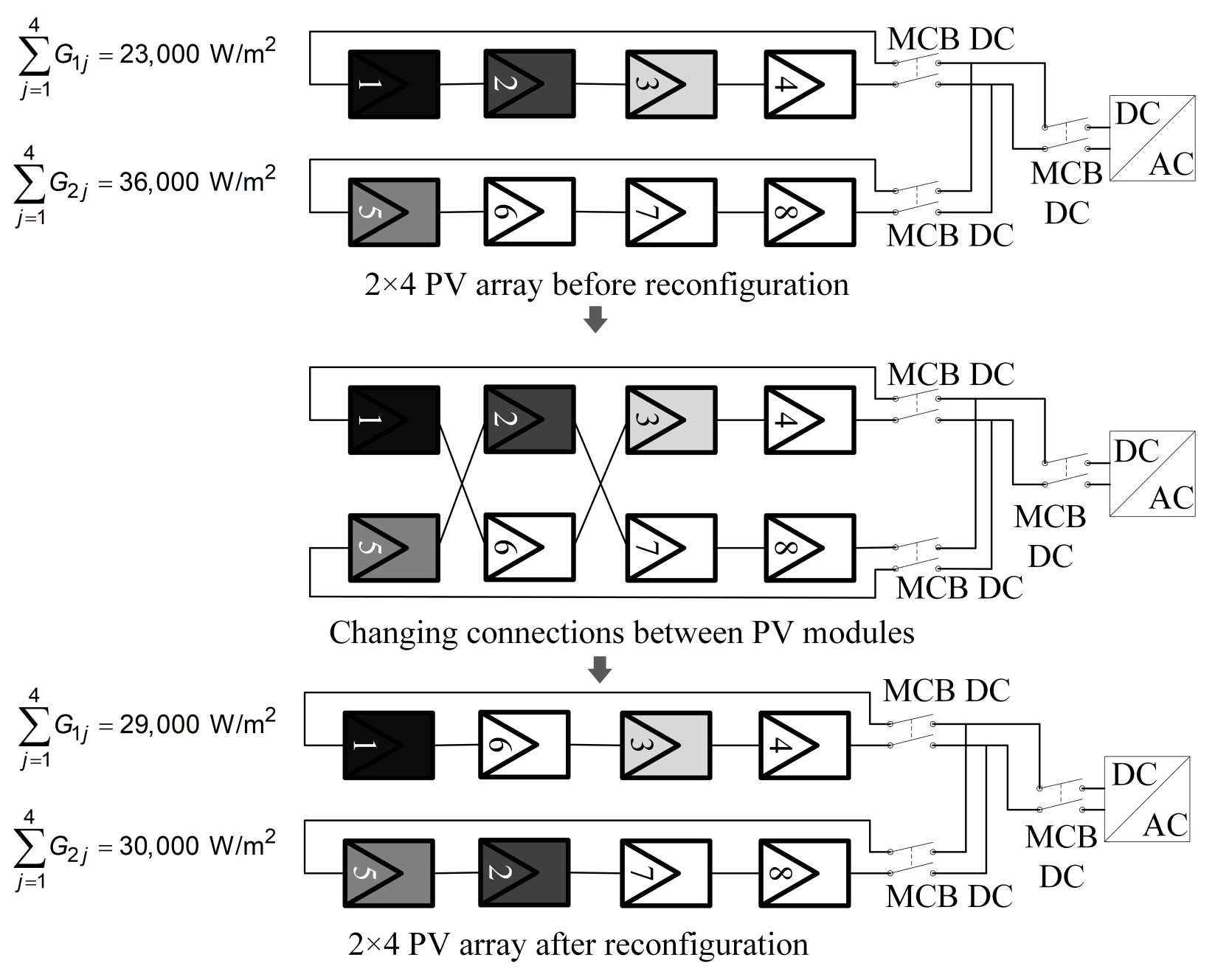
To increase the output power and reduce the number of local MPP on the power-voltage curve of the PV array under PSC, the principle of irradiance equalization is proposed, which aims at equally dispersing total irradiance on rows of PV modules [9]. In DPVAR, this principle is attained by changing the terminal connections of the PV modules without altering their wires. An example of irradiance equalization is illustrated in Figure 2. Under PSC, the difference between the total irradiance on the first row and the second row is 13,000 . After changing the connections of PV module 2 and PV module 6 with adjacent PV modules, this difference is reduced to 1000 . The optimal configuration for the PV array under PSC is determined by the RA.
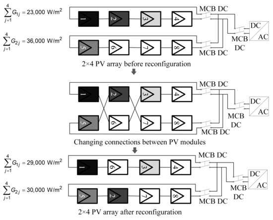
Figure 2.
Principle of irradiance equalization of DPVAR.
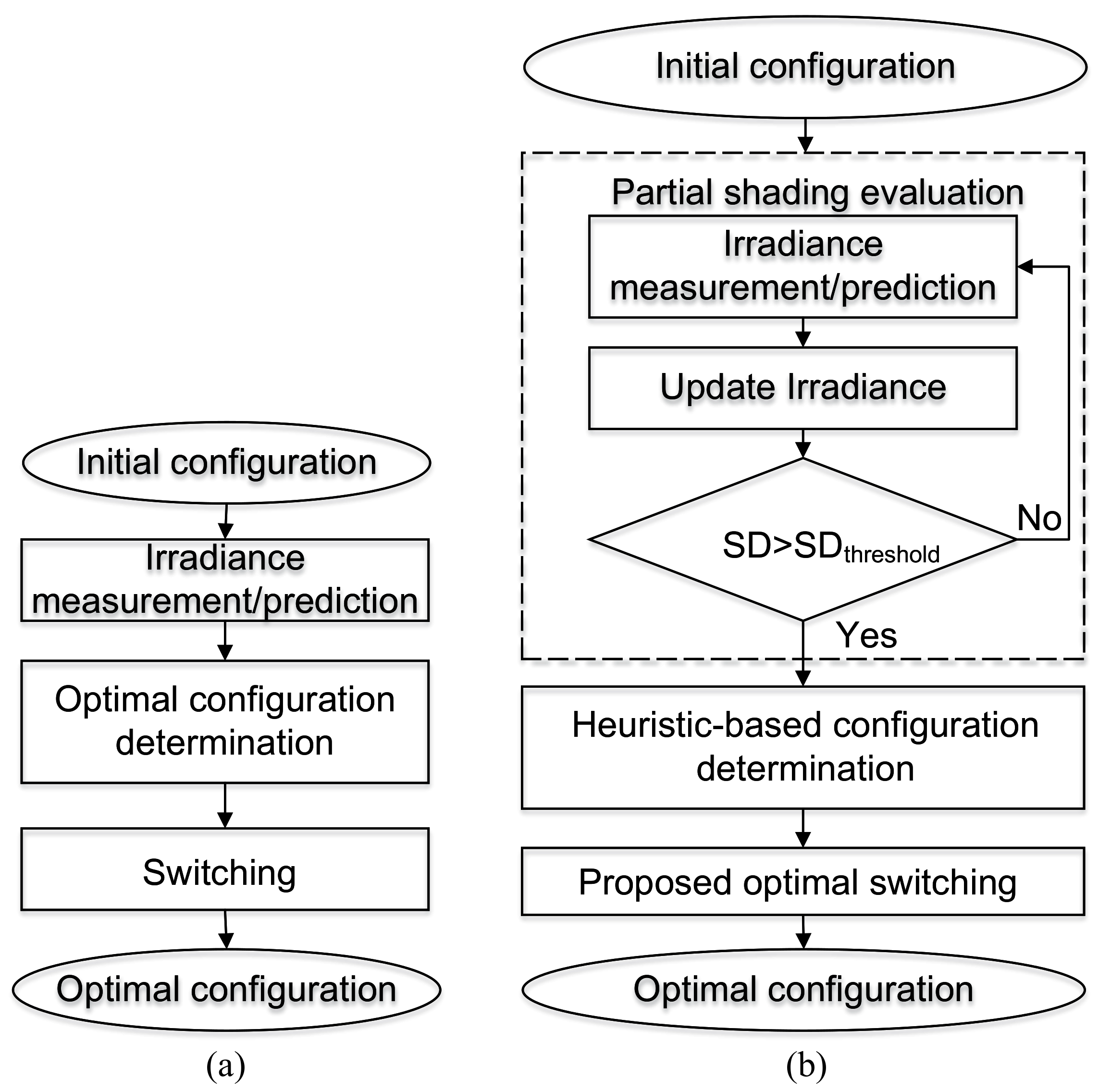
Figure 3a describes a general process of the DPVAR strategy, which can be divided into three steps as follows:

Figure 3.
(a) Traditional DPVAR framework. (b) Proposed DPVAR framework.
- Irradiance measurement/prediction: The irradiance data on PV modules are typically measured by pyranometers. However, this approach is costly, as it requires a pyranometer for each PV module. An alternative approach in [9,18] predicts the irradiance of the measured current of each PV module. Although this method can leverage the available data from the inverter, the predicted irradiance values are lagged behind the occurrence of PSC. Therefore, the effectiveness of the RA is diminished.
- Optimal configuration determination: An optimal configuration of a PV array under PSC is defined as having the most equally distributed irradiance on rows of PV modules. To evaluate the performance of a solution, the fitness function is to minimize the standard deviation (SD) of the irradiance on rows of PV modules of the PV array:where m is the number of rows of the PV array, is the total irradiance of PV modules in the row, and is the average value of total irradiance on each row of the PV array.
- Switching: After finding the optimal configuration, the switching matrix controls the changes in electrical connections between PV modules.
3. Proposed Methodology
The conventional DPVAR process in Figure 3a is applicable for only the single-time step operation since the RA does not specifically indicate whether the DPVAR should be deployed. In addition, three steps, 1–3, could still be improved to enhance the accuracy of irradiance prediction, obtain optimal PV array configuration, and optimize the switching operation. The first step can be conducted with irradiance measurement or estimation on each PV panel in the array. The second step can be solved by a reconfiguration algorithm. Many types of research were published to adapt the arrangement of PV modules to various partial shading patterns. The switching board modifies the connection between PV modules to achieve the final arrangement in the last step. In this paper, a novel framework is proposed for the continuous operation of the DPVAR (Figure 3b). In the irradiance measurement/prediction step, a method is developed to extract the irradiance data from the synthesized image of the MC. As the electrical connections between PV modules could be changed during the operation, the input irradiance is updated based on the extracted irradiance matrix and the current PV array configuration. To evaluate the level of the PSC, a threshold of the SD of irradiance (SDI) on rows of PV modules is set. If the SDI on the PV array exceeds its threshold, then RA will be activated. Otherwise, the PV array will remain its current configuration. In the step of finding optimal configuration, improved PSO-based and Rao-based RA are proposed. Finally, the switching operation is optimized by a PSO-based process.
3.1. PSC Evaluation
The PSC evaluation is accomplished to predict the irradiance on the PV array’s surface, determine irradiance on each PV module when considering the previous reconfiguration, and establish a threshold for activating DPVAR.
3.1.1Extract Irradiance Matrix from Images of MC
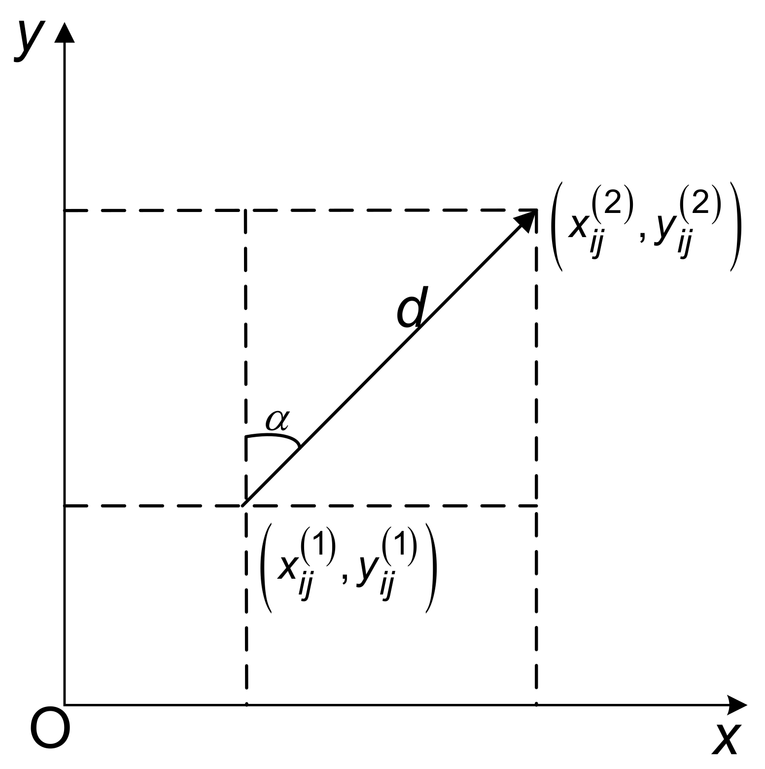
To study the operation of the DPVAR in continuously changing shade, the MC is emulated by utilizing the synthesized image of the cloud from [22] (Figure 4). This image is of pixels, which captures an MC with the size of m. This size of the MC is far larger than the typical size of the PV array. Therefore, the irradiance on each PV module can be determined by projecting the PV array on the shade. In other words, the irradiance level of the PV array can be expressed by its coordinate on this projection. The brightest pixels on the image are referred to as the irradiance on PV panels without any shading, and the darkest is a tenth of the brightest. Following various studies in the literature, the irradiance on unshade modules is taken as a common value of 1000 W/m. The transition of two consecutive irradiance situations on the PV array is simulated by two matrices, whose entries are coordinates of the PV modules on the projection (in (5)). From this coordinate matrix, the irradiance matrix is obtained by referring to cloud irradiance. In (6), the coordinate of a PV module is updated based on the direction and the moving distance of the cloud (Figure 5). Whereas d is the distance of MC in a sampling time and is the angle of the direction of the MC. Herein, the sampling time is set to 1 s.
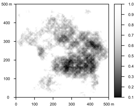
Figure 4.
A synthesized image of studied cloud. Reprinted/adapted with permission from Ref. [22]. 2020, Chen et al.

Figure 5.
Transition of the coordinate of PV module on projection of MC.
Note that the extracted irradiance matrix is not the input irradiance matrix for the RA. In continuous operation, the current configuration of the PV array needs to be considered to determine the actual irradiance for each PV module.
As the SDI is always greater than zero under operating conditions, it is necessary to set an activated threshold for the SDI to decide whether the reconfiguration is deployed. If the activated threshold of SDI is set too low, the power will be enhanced at the expense of high switching times. As the threshold of the SDI profoundly depends on the characteristic of the shading [27], herein, the activated threshold of the SDI on the PV array is determined by using the trial-and-error method during the simulation process.
3.2. Proposed Reconfiguration Algorithms
Determining the optimal configuration for the PV array is an NP-hard problem [11] as the number of possible solutions for choosing connections for PV modules of the PV array is gigantic. Given a TCT PV array, the number of solutions is 81-factorial, therefore, methods such as brute force, are not feasible. In recent, heuristic algorithms have shown their superiors for NP-hard problems since heuristic algorithms always give the near-global optimal solution. Studies [14,18] implement PSO and Rao algorithms to obtain the optimal configuration for the PV array under PSC. However, the models in [14,18] are roughly implemented PSO and Rao algorithms, however, they are not specifically stated for the DPVAR problem. In our DPVAR model, three techniques, including inertia weight adapting, population diversifying, and low-quality-solution screening, are proposed to enhance the performance of the searching algorithms.
Improved PSO Algorithm
PSO algorithm [28] mimics the cooperation of the flock of birds in foraging for food. To find the best place for food, an individual will decide which position to land based on three pieces of information: its current position, the best position based on its experience, and the best position based on the flock experience. This behavior inspires the updating mechanism of the PSO algorithm, which is expressed as follows:
where and are the velocity of the particle (bird) in the and iteration (two consecutive landings), respectively. w is the inertia weight (its current position), and is the uniform distribution between 0 and 1. is the best position of the particle in the past (bird’s experience), and is the position of the best particle in the population (experience of the other bird in the flock). and are positions of the particle (two consecutive places) in the and iteration, and are the personal and global learning coefficients.
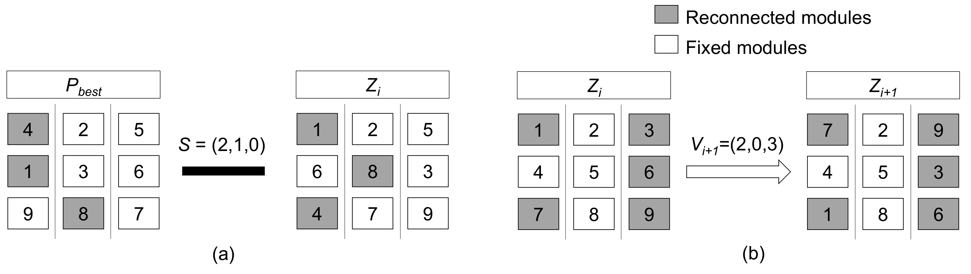
When applying the PSO algorithm to the DPVAR, (7) and (8) should be defined carefully to exploit the learning capability of the algorithm fully. The subtraction of the particle’s positions, and in (7), are determined by comparing two PV configurations utilizing the vector of comparison S (stands for Subtract) (Figure 6a). Each entry of S determines the degree of difference between two configurations and is initially set to zero. When comparing each column of two PV configurations, an entry of the S vector is added by 1 when a module in that column is not found in the respective row of the compared configuration. This comparison process can be illustrated by a simple example in Figure 6a:
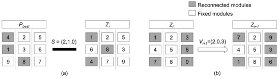
Figure 6.
(a) Example on comparing two PV configurations. (b) Example on updating PV configuration.
- When comparing column 1 of configuration 1 to column 1 of configuration 2, module 4 located in row 1 of configuration 1 does not appear in row 1 of configuration 2; module 1 (row 2, configuration 1) does not appear in row 2 (configuration 2); module 9 (row 3, configuration 1) appears in row 3 (configuration 2). Therefore, the first element of S is set by 2.
- For column 2 of configuration 1, module 2 (row 1, configuration 1) and module 3 (row 2, configuration 1) appear in row 1 and row 2 (configuration 2), respectively; module 8 does not appear in row 3 (configuration 2). Therefore, the second element of S is set by 1.
- For column 3 of configuration 1, all modules are found in respective rows of configuration 2. Therefore, the third element of S is 0.
is also defined in a similar way via vector S.
When a particle approaches closely to its optimal position, its velocity reduces over iterations. Therefore, the inertia weight w is expressed as a function of the current iteration i as follows:
where and are the inertia weights in the first and the last iterations, and is the maximum number of iterations. When increasing i from 1 to , w would be decreased from to . This means that the rate of changing the inertia weight is decreased, which means the number of PV modules being reconnected in a configuration is reduced when the obtained configuration approaches closely to the most optimal one.
The velocity vector V is used to present the number of reconnected PV modules of the PV array. Each entry of V stands for the number of PV modules in each column being reconnected. New connections are chosen stochastically in the PV array. After determining the vector V, the addition in (8) is defined by updating the new PV configuration Z. Figure 6b shows a simple example of updating Z via its velocity vector V:
- The first entry of the velocity vector , therefore, two modules in column 1 are randomly chosen and reconnected.
- The second entry of the velocity vector , so all modules in column 2 are remained.
- The third entry of the velocity vector , so all three modules in column 3 are randomly reconnected.
The processes of comparing and updating the PV array configuration based on the PSO algorithm are rewritten as follows:
In [18], the population of the PSO algorithm is created only by changing the connections of PV modules in the same column. This column-wise initialization of the population limits the learning capability of the algorithm. For instance, a PV module cannot be switched to another module in the same row. Therefore, in certain shading patterns, the searching domain is limited. In the proposed algorithm, the population is created by switching PV modules across the PV array.
In addition, to prevent low-quality solutions from being generated, each solution is compared with the previous one and will be removed if its fitness value exceeds the fitness values of the previous solution by . The following pseudo-code is used to decide whether a new configuration is updated or removed.
The above-elaborated process is summarized into three following steps:
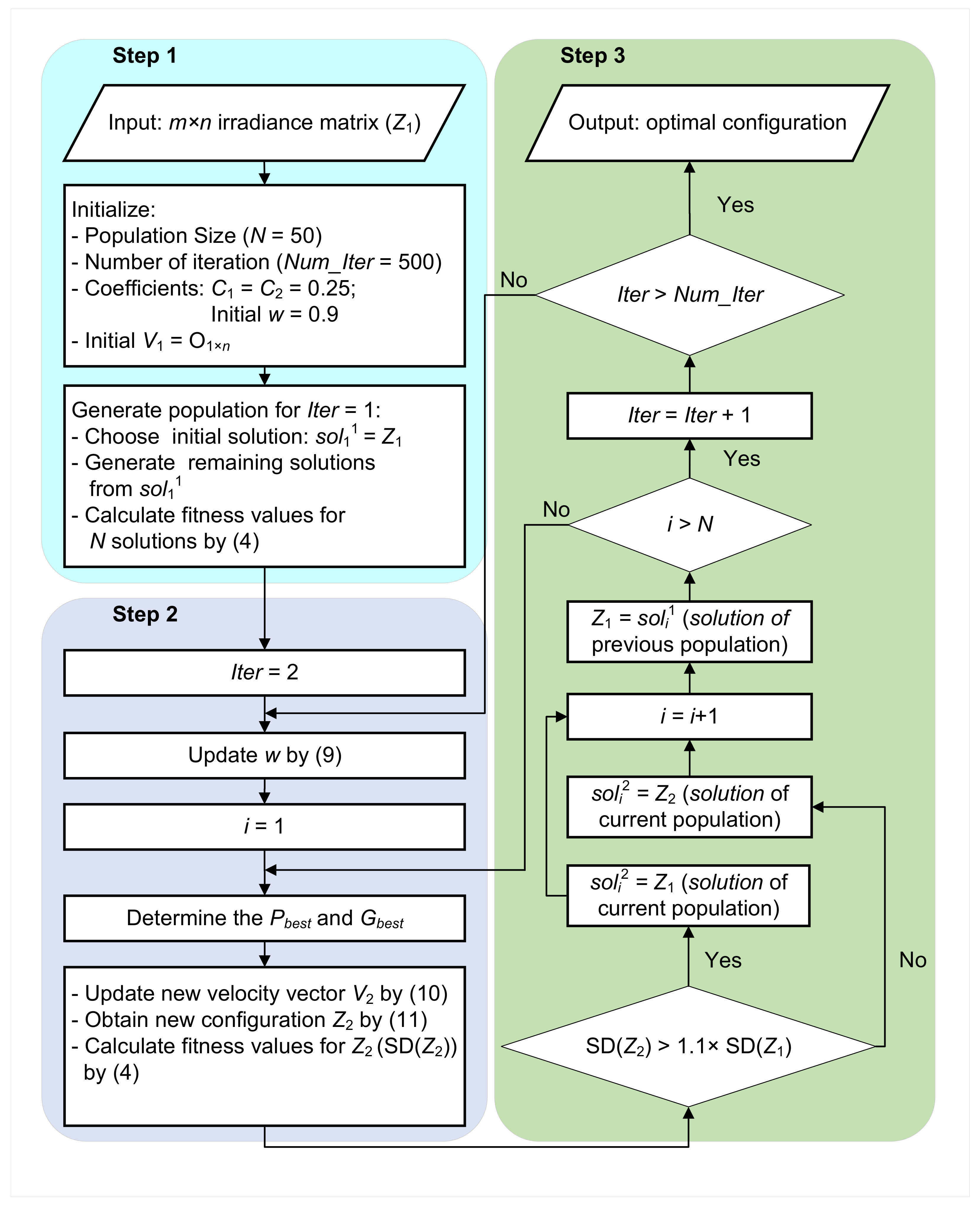
- Step 1: Initialize the algorithm’s parameters and generate the first population.The irradiance matrix of the PV array is entered. The algorithm parameters are initialized including population size (N), the number of iterations (), personal and global learning coefficients ( and ), and the initial inertia coefficient (w). The initial updating vector is set to zero vector (n entries correspond to n columns). After that, population 1, which corresponds to iteration 1 ( = 1), is generated. The initial solution of population 1 ( s.t. i = 1) is . The remaining solutions of population 1 are generated from by stochastically changing modules across the PV array. The fitness values of each solution of population 1 are calculated by (4).
- Step 2: Update new populations.
- Step 3: Evaluate new populations and determine the most optimal configuration.The new solution is evaluated based on Algorithm 1. The solution of population 2 () remains to if , otherwise it is updated by . After determining solution 1 for population 2, the remaining solutions for population 2 are found in a similar way. is assigned to the solution i of iteration 1 ().After obtaining all solutions for population 2, the remaining populations are determined in the same token as done for population 2. The optimal configuration is the best of global solutions for all populations.
The proposed PSO-based RA is represented by the flowchart in Figure 7.
| Algorithm 1 Screening low-quality solutions. |

Figure 7.
Flowchart of proposed PSO-based RA.
3.3. Improved Rao Algorithm
Rao [29] is a teaching-learning-based algorithm, which only requires initializing the size of the population and the maximum number of iterations. Since the Rao algorithm does not require any parameters for the algorithm, its performance is less dependent on initial parameters. The original updating equations of the Rao algorithm are expressed as follows:
where is the attribute of the considered candidate in the iteration, is the uniform distribution between 0 and 1. and are the solutions given by the best and the worst candidates, respectively. is the solution of the randomly picked candidate. and are the solutions of candidate Z at the and iterations, respectively.
The subtraction vectors and in (12) are also calculated based on the vector of comparison S, which is previously described in Figure 6a. The process of updating the PV configuration described in (13) is determined as the same as the example in Figure 6b. Therefore, the PV array configuration is updated in the same way as for the proposed PSO algorithm:
The process of the proposed-Rao-based RA is done as same as the proposed-PSO-based RA without initializing coefficients of the algorithm (, , w) and updating w.
3.4. Optimal Switching Procedure
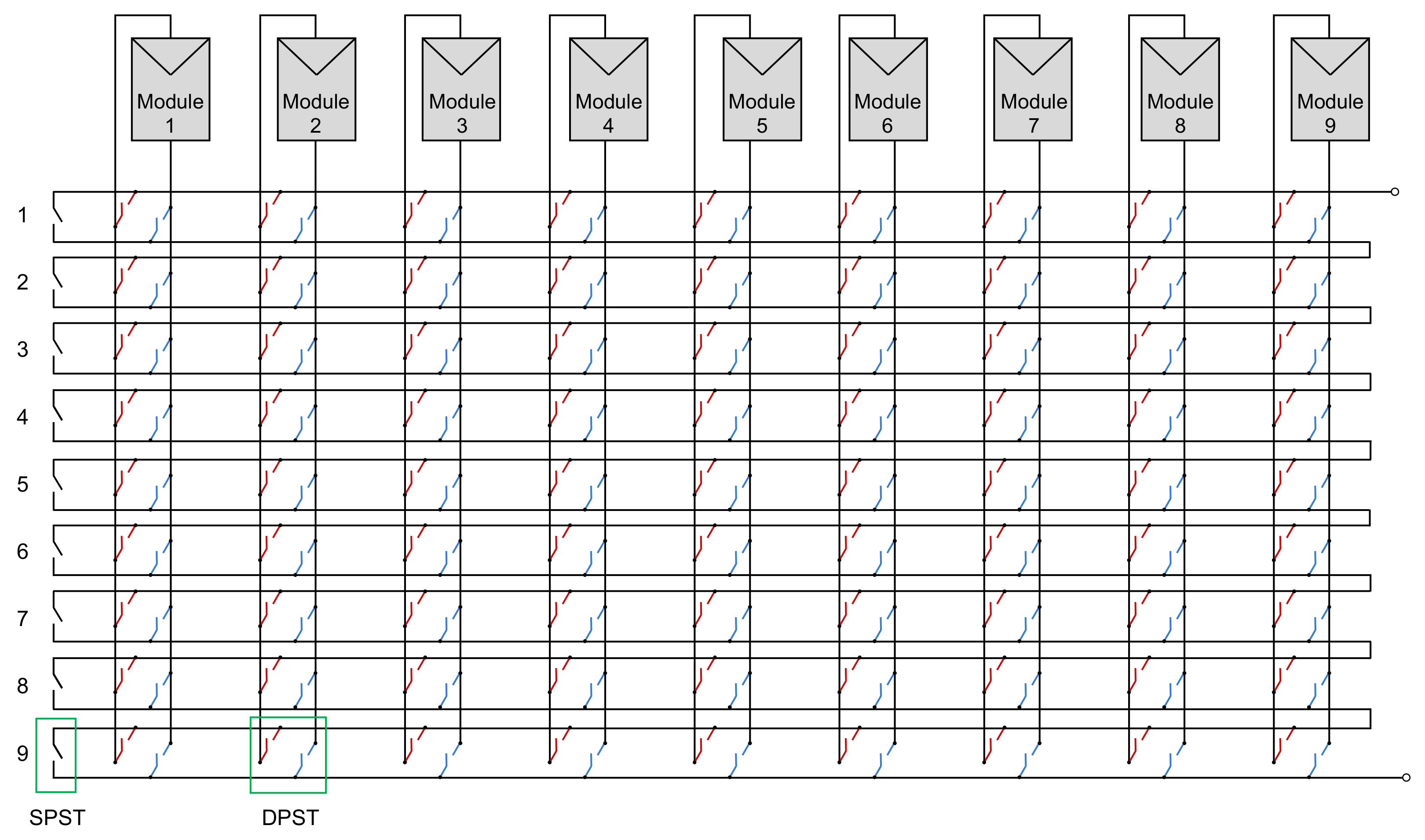
In DPVAR, the switching board is controlled by the RA to change terminal connections of PV modules in the PV array. This study utilizes the DES (Figure 8) proposed by [21] for DPVAR on an PV array. This structure of the DES ensures that a PV module in the PV array can be rearranged to any position across the PV array as the proposed RA intends. Furthermore, the single-pole-single-throw and double-pole-single-throw switches have already been sold commonly.
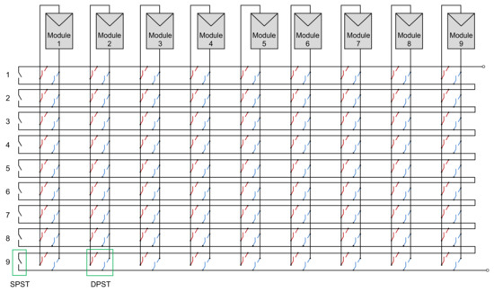
Figure 8.
Dynamic Electrical Scheme. Reprinted/adapted with permission from Ref. [21]. 2013, Romano et al.
This paper proposes a procedure to count the number of switches needed to change the PV array from the initial configuration to the optimal one and identify the activated switches based on the DES. Firstly, an matrix of operating switches C is created to determine switches that are changed their states from closed to opened and vice versa. The columns represent the PV modules, and the rows are used to determine the working state of double-pole single-throw (DPST) switches that connect the modules to the corresponding rows of the array. For instance, when and , two of the m switches, which are connected to the PV module, operate to change connections of this module with row and row to intended rows. Secondly, the switch tracking process (STP) is developed to determine the properly activated switches. This STP is described as follows:
- STP starts from row 1 to row m of the optimal configuration.
- For row 1, STP starts from module 1 to module n to obtain a module in the initial configuration (called the matching module) that has the same irradiance level as the considered module in the optimal configuration. When a matching module is found, it will be removed from the searching set to ensure that it is not tracked again in the next iterations. If the matching module is found in row 1, STP moves to the next module in the optimal configuration without any change in the matrix C. If no matching module is found in row 1, STP continues with row 2, row 3, etc. When the matching module is found, for example in row j of the initial configuration, the considered module is reconnected from row j to row 1, so that two corresponding switches in row j and row 1 of this module are opened and closed consequently.
- For row 2, STP is prioritized from row 2 of array 1. If the matching module is not found in row 2, STP returns to search from row 1. Note that the respective row is prioritized to search first. If the row respective row does not have the matching one, then STP is considered from row 1 to row m.
- STP for row 3 to row m are completed as for row 2.
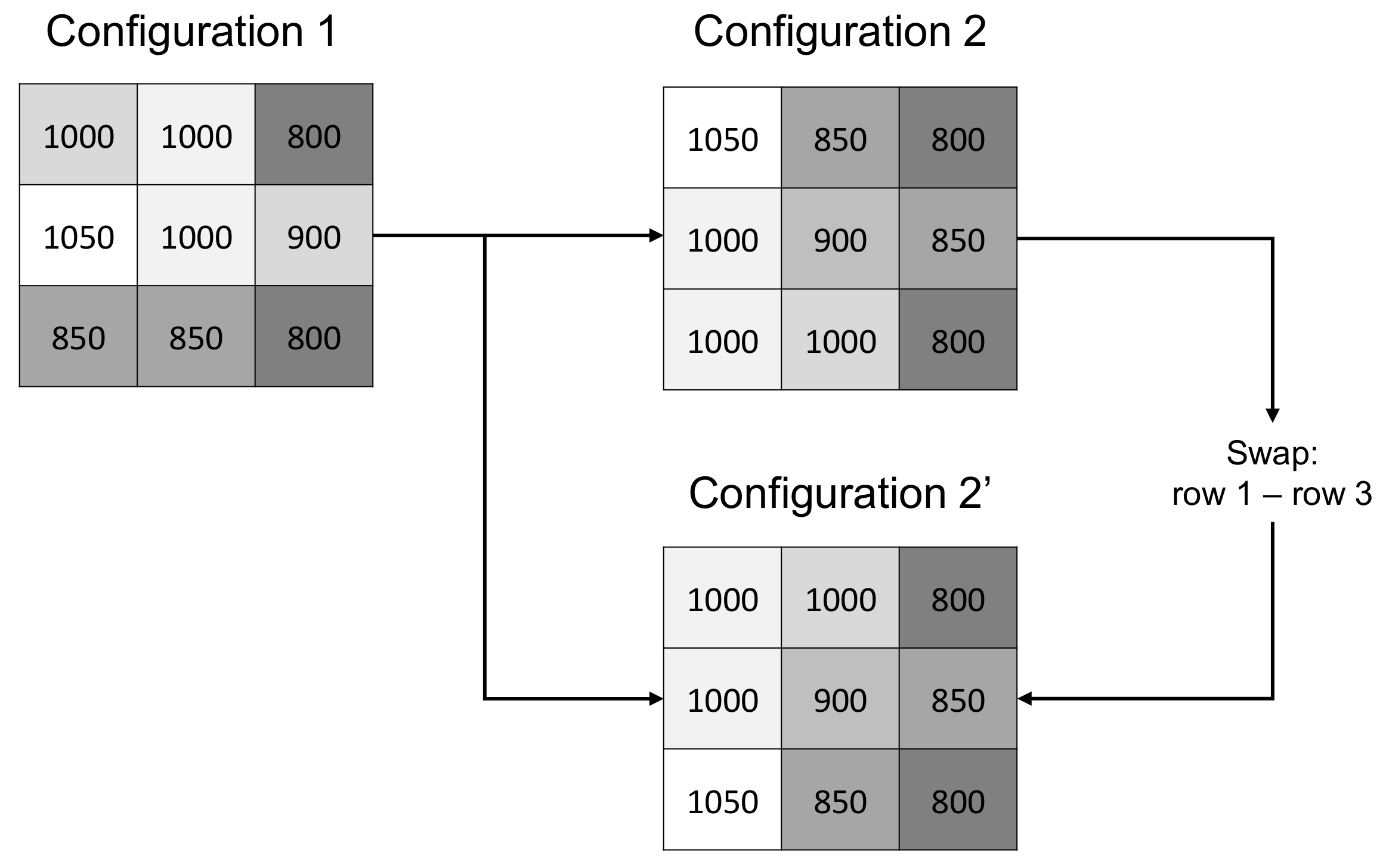
The above STP ensures that a module does not need to be switched if there is a matched module in the same row at the initial configuration. However, the switching times can be more optimized by changing the rows of optimal configuration. Figure 9 shows an example of two different optimal configurations (2 and 2), which are rearranged from the same initial configuration 1. Table 1 summarizes the operating switches matrix (the module is abbreviated as Mi) of the STP on the PV array in Figure 9. It can be seen that configuration 2 requires 6 switching times less than configuration 2 does.

Figure 9.
Example of two optimal configurations solved from an initial configuration.

Table 1.
Matrix of operating switches and corresponding to two optimal configurations 2 and 2.
In practice, DPVAR operates continuously under PSC. The aging of the switching matrix is dependent on not only the total switching times of all switches but also the operating times of the active switches. This is because when a switch is broken, the whole switching matrix needs to be maintained. Therefore, the switching operation should be uniformly distributed for all switches. In this paper, a PSO-based switching optimization algorithm is performed to reduce the total number of switching times and to limit the operation of the most active switches. The objective function for optimal switching operation is:
where is the total number of switching times of the switch from being installed, is the binary status of the switch, which is summarized from C. It is noteworthy that for the active switches that have high , the objective function aims to let their status, , will less likely to be 1. For the parameters of the PSO-based switching optimization algorithm, the number of the population is 50, the personal learning coefficient and the global learning coefficient are set to 0.25, and the initial inertia coefficient is set to 0.9.
4. Results and Discussion
The proposed DPVAR model is validated on two following operational modes:
- Single-time step operation: The performance of the PSO-based and Rao-based RA are validated under three PSC patterns, which consider the PV array is under the center of the cloud, under the top edge of the cloud, and under the right edge of the cloud. Three performance metrics are utilized, namely global MPP (GMPP), power enhancement (PE), and power losses (PL), to evaluate the performance of the proposed PSO and Rao algorithms against the original PSO and Rao algorithms. GMPP is the global peak of the P-V curve of the PV array. PE and PL are calculated by (17) and (18) [14], respectively.where is the maximum power of the TCT PV array under PSC, is the maximum power of the PV array with the considered configuration under PSC, and is the maximum power of the TCT PV array under non-PSC.
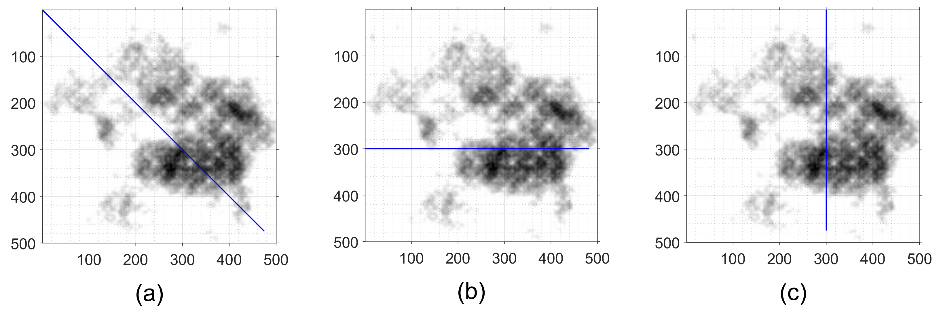
- Continuous operation: In this operational mode, the PV array is investigated under an MC, whose properties are varied. As the operation of the DPVAR is continuous, the processing time of the reconfiguration process will affect the overall performance of the DPVAR. The proposed method to extract irradiance in Section 3.1.1 could provide the irradiance profile on the PV array before happening PSC. Therefore, the RA could be processed before the time of PSC, then the physical reconfiguration process will be deployed at the time of PSC. This scenario of operating the DPVAR is called DPVAR without time lagging. If irradiance is measured/predicted at the same time as the PSC, the physical reconfiguration process will be lagged behind PSC. This scenario of operation is called DPVAR with time lagging. Herein, the lagged time is set to 1 s, as the processing time of the original PSO and RAO algorithms are about 1 s [18]. The activated of the SDI is set equal to 300 and 200 for the scenarios without and with time lagging, respectively. This difference in the threshold of the SDI ensures that the power improvement in the two scenarios is not so deviated.For the MC’s properties, three case studies of the MC are presented in Figure 10. The speed of the cloud is set to 15 m/s, which is the most sensitive case for triggering PV power fluctuation [22]. The direction of the cloud is modeled by three patterns: moving across the PV array, moving horizontally the PV array, and moving vertically the PV array. The effects of partial shading on the PV array are different with each pattern. The vertical direction of the cloud made the standard deviation of irradiance on rows to be high; therefore, the power improvement is most considerable after reconfiguration. Whereas, the horizontal pattern of the cloud is the least negative. The reconfiguration method also shows less effect in this case. As the MC is very large compared to the PV array, the thickness, shape, and size of the MC-induced shade also continuously varied during the time the MC passed on the PV array. Aside from evaluating the power optimization of the PV array, the switching operation is also verified in terms of the total number of switching times and the frequency of the active switches.
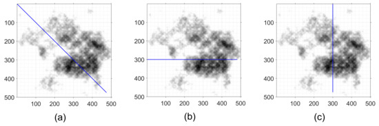 Figure 10. Three case studies of MC on studied PV array (The blue lines show directions of the MC). (a) Case 1. (b) Case 2. (c) Case 3.
This study utilizes a multi-crystalline silicon PV module, whose specification in the Standard Test Conditions (irradiance is 1000 , temperature is 25 C) is provided in Table 2.
Table 2.
Specification of PV Module at Standard Test Condition [30].
4.1. Operation of Proposed DPVAR on Single Time Step
4.1.1. PV Array under Center of MC
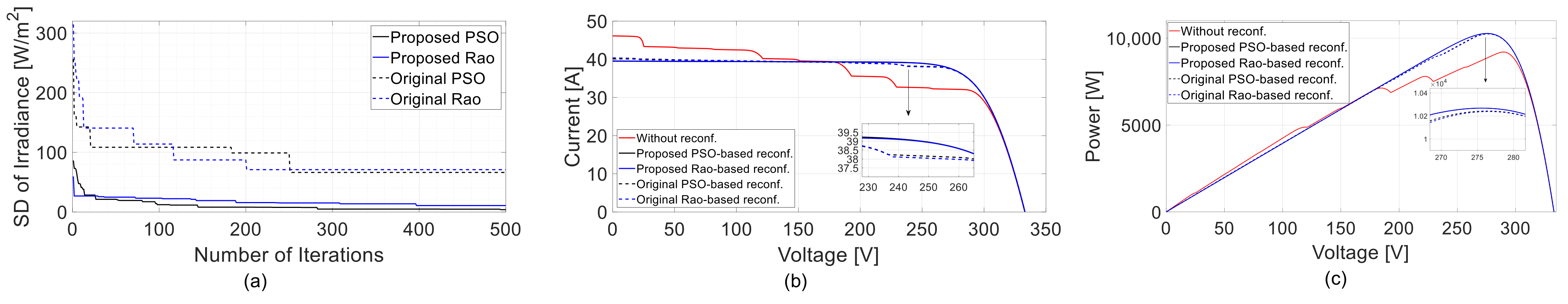
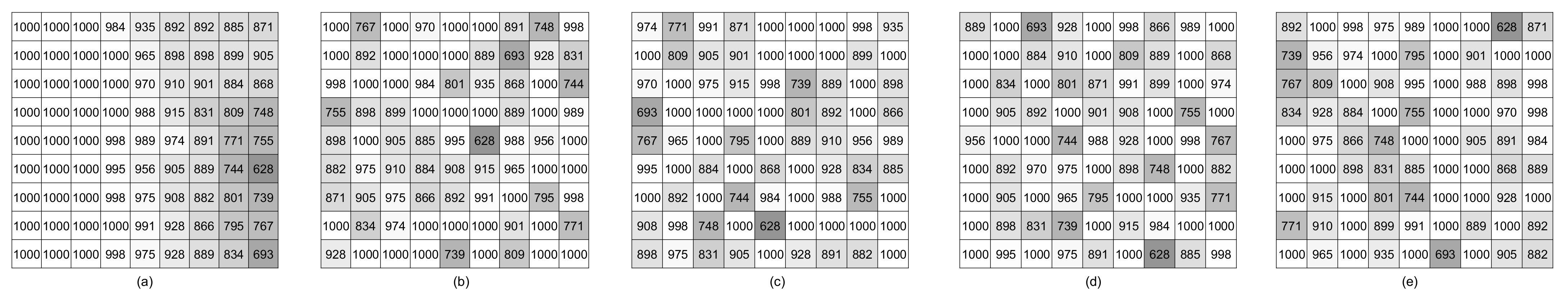
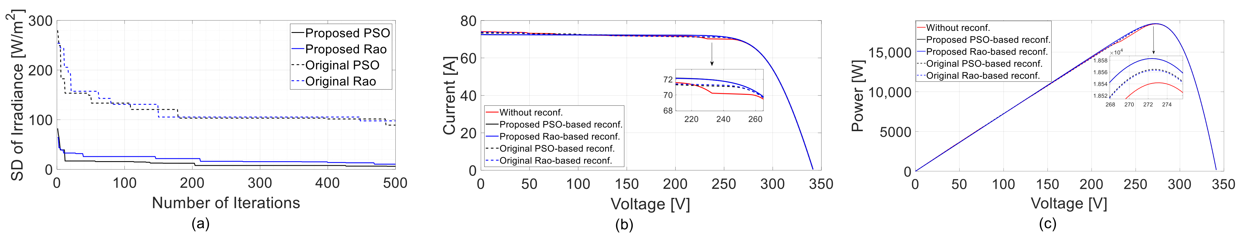
Figure 11 presents the irradiance distribution of the PV array under the center of the cloud before the reconfiguration, after the original and proposed DPVAR. The low-irradiance areas previously located at the right-bottom corner are dispersed to different modules across the PV array after the reconfiguration. Figure 12a shows the SDI on the PV array over iterations. The initial values of the SDI of the proposed RA are much lower than the ones of the original RA. This shows the effectiveness of the proposed initialization method over the column-wise initialization method. At the last iteration, the SD on the PV array with the proposed-PSO-based (4 ) and the proposed-Rao-based (11 ) configurations are lower than the ones on the PV array with the original PSO-based (66 ) and Rao-based configurations (71 ). Figure 12b,c present the comparison between the I-V curves and P-V curves of the PV array without the reconfiguration, with the original RA, and with the proposed RA. The I-V curves of the proposed-PSO-reconfigured PV array and the proposed-Rao-reconfigured PV array appear with no “steps”, while the ones with the original-PSO-reconfigured and original-Rao-reconfigured PV arrays still appear “steps” at the vicinity of the MPP (Figure 12b). The P-V curves of the PV array with the proposed PSO and Rao algorithms have higher peaks than the PV array with the original PSO and Rao algorithms have (Figure 12c). The P-V curves of the proposed-PSO-reconfigured PV array and the proposed-Rao-configured PV array are almost overlapped. To be more specific, the GMPP, the PE, and the PL of the PV array are illustrated in Figure 13. The GMPP of the proposed-PSO-reconfigured PV array is 25 W higher than that of the original-PSO-reconfigured PV array, while the proposed-Rao-reconfigured PV array is 30 W higher than that of the original-Rao-reconfigured PV array (Figure 13a). Consequently, the proposed PSO and Rao configurations achieve a higher PE (Figure 13b) and suffer less PL (Figure 13c) compared to other configurations do.
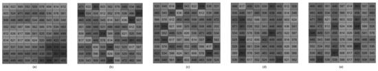
Figure 11.
Shading distribution on PV array under the center of the cloud. (a) Before reconfiguration. (b) After original-PSO-based reconfiguration. (c) After the original-Rao-based reconfiguration. (d) After the proposed PSO-based reconfiguration. (e) After the proposed-Rao-based reconfiguration.
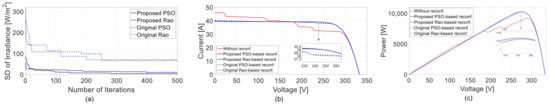
Figure 12.
Comparison of characteristics of PV array under the center of the cloud. (a) Objective function over iterations. (b) I-V curves. (c) P-V curves.
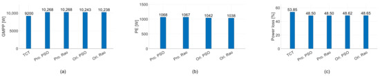
Figure 13.
Comparison of performance metrics of PV array under the center of the cloud. (a) GMPP. (b) PE. (c) PL.
4.1.2. PV Array under Top Edge of Cloud
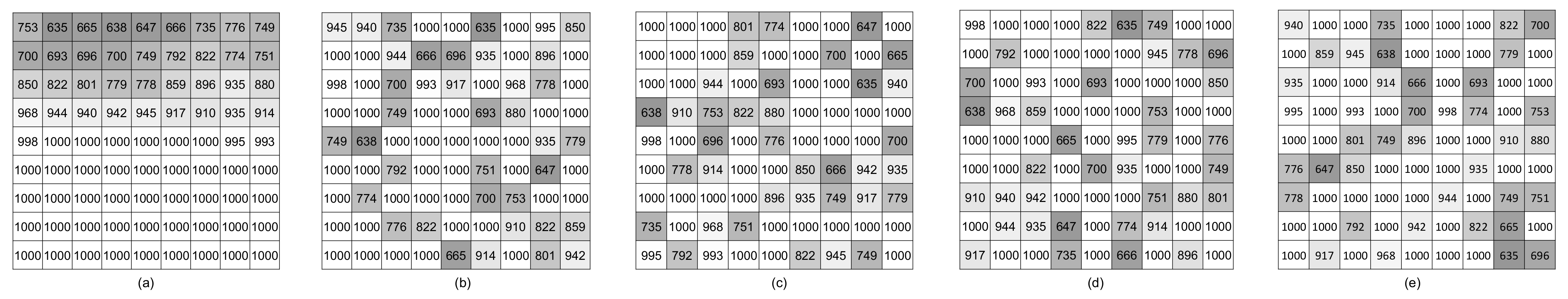
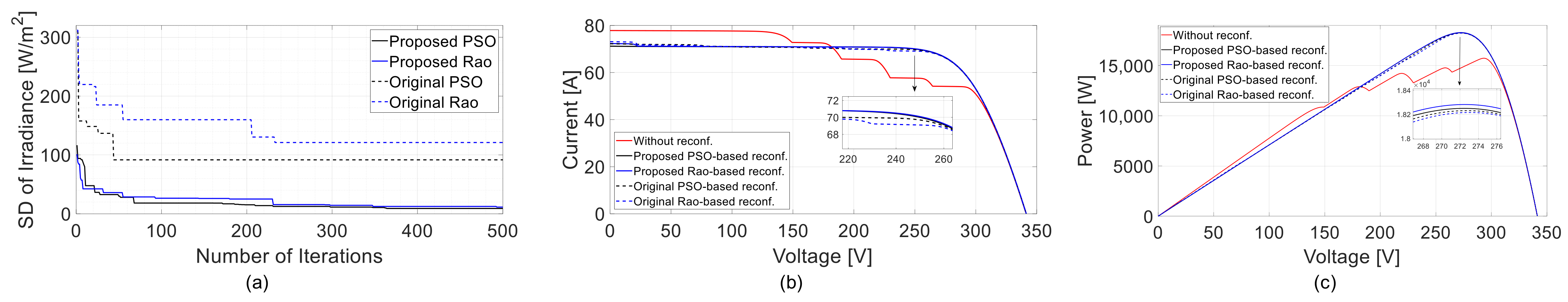
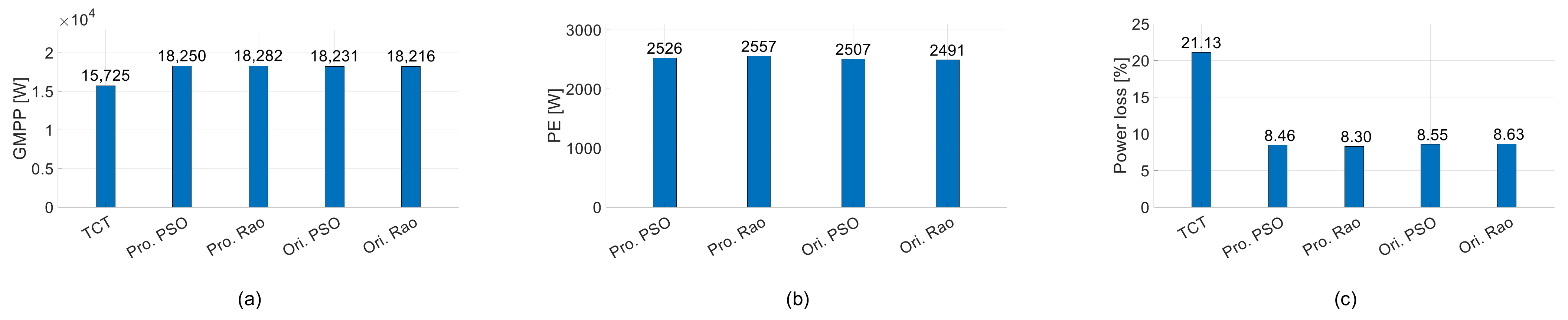
Analogously to the PV array in the center of the cloud, after the reconfiguration, the PV array under the top edge of the cloud has a better equal distribution of irradiance, as the PV modules with low irradiance on the top edge of the PV array receive a higher irradiance after reconfiguration (Figure 14). The proposed PSO and proposed-Rao algorithms provide the PV array with a lower SDI compared to the original algorithms (Figure 15a). The I-V curves of the proposed and original algorithms are smooth in the areas near the MPP point (Figure 15b). The TCT-configured PV array only reaches 15,725 W and suffers a PL of 21.13% (Figure 16). The proposed-Rao-reconfigured PV array has the highest GMPP (18,282 W), the highest PE (2557 W), and its PL is significantly reduced from 21.13% to 8.30% after reconfiguration (Figure 16).
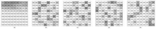
Figure 14.
Shading distribution on PV array under the top edge of the cloud. (a) Before reconfiguration. (b) After the original PSO-based reconfiguration. (c) After original-Rao-based reconfiguration. (d) After the proposed PSO-based reconfiguration. (e) After proposed-Rao-based reconfiguration.
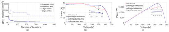
Figure 15.
Comparison of characteristics of PV array under the top edge of the cloud. (a) Objective function over iterations. (b) I-V curves. (c) P-V curves.

Figure 16.
Comparison of performance metrics of PV array under the top edge of the cloud. (a) GMPP. (b) PE. (c) PL.
4.1.3. PV Array under Right Edge of Cloud
Under the right edge of the cloud, the difference in the total irradiance on the rows of the PV array before and after the reconfiguration is not significant as the PV array under the center and the top edge of the cloud. This is because the low-irradiance areas under the right edge of the cloud are already located in a row-wise manner on the PV array (Figure 17). The proposed-PSO-reconfigured and proposed-Rao-reconfigured PV arrays give the lowest SDI (Figure 18a), the smoothest I-V curves (Figure 18b), and the highest peaks on the P-V curves (Figure 18c). The GMPP, the PE, and the PL of the proposed reconfigured PV arrays are better than those of the TCT and original reconfigured PV arrays (Figure 19). It can be seen in Figure 19c that the right edge of the cloud does not much affect the output power of the PV array as the center and top edge of the cloud do.
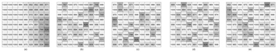
Figure 17.
PV array under the right edge of the cloud. (a) Before reconfiguration. (b) After original-PSO-based reconfiguration. (c) After the original-Rao-based reconfiguration. (d) After the proposed PSO-based reconfiguration. (e) After the proposed-Rao-based reconfiguration.
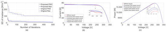
Figure 18.
Comparison of characteristics of PV array under the right edge of the cloud. (a) Objective function over iterations. (b) I-V curves. (c) P-V curves.
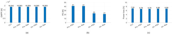
Figure 19.
Comparison of performance metrics of PV array under the right edge of the cloud. (a) GMPP. (b) PE. (c) PL.
4.2. Operation of DPVAR on Continuous Time Steps
4.2.1. DPVAR without Time Lagging
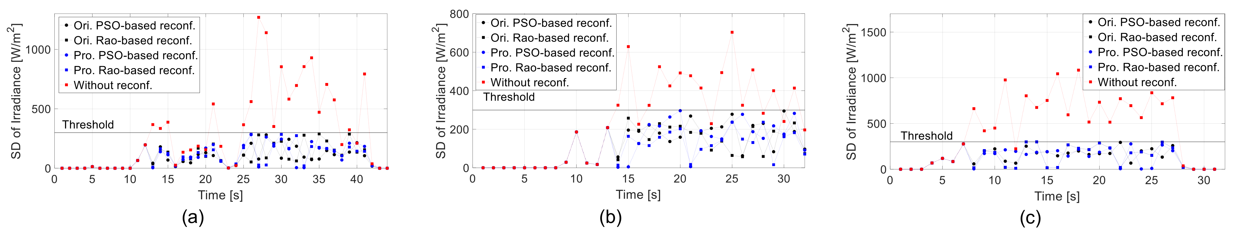
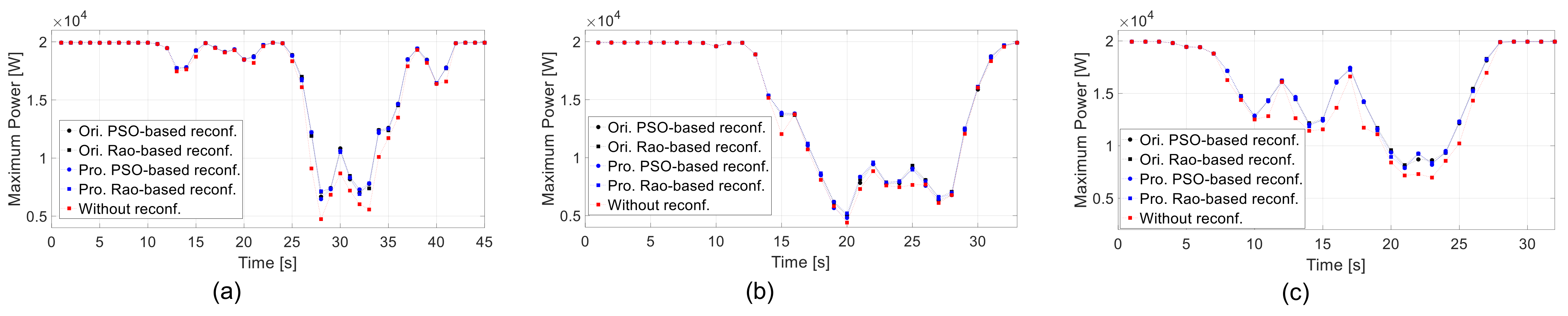
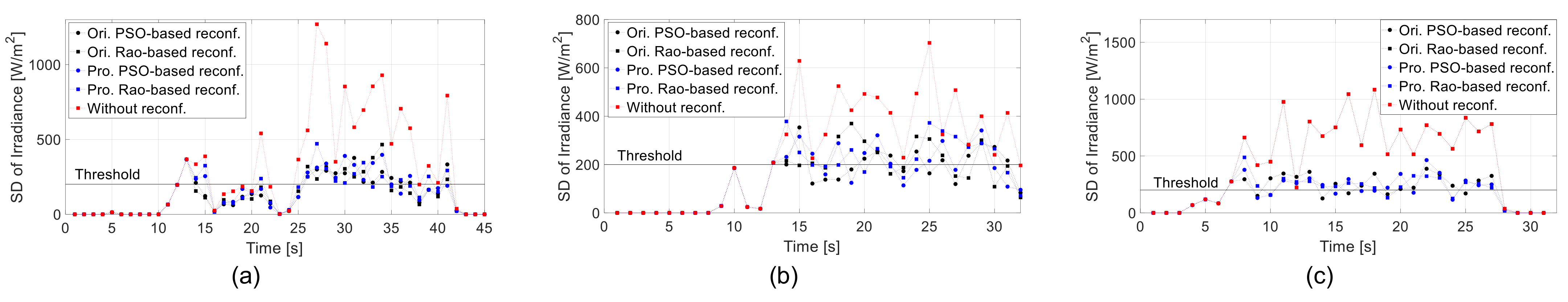
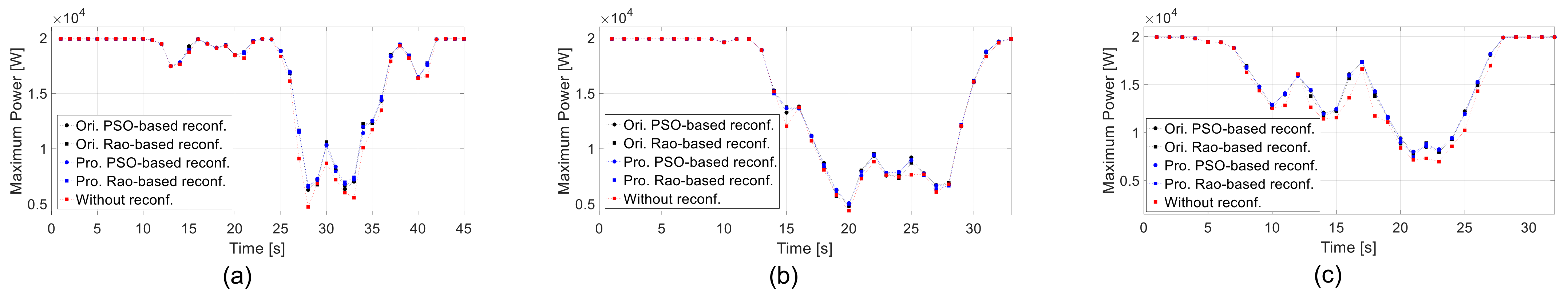
Figure 20 displays the SDI of the PV array without the DPVAR, with the original and proposed DPVAR. It can be seen that the proposed reconfigured PV arrays have highly fluctuated SDI profiles in all three MC patterns. This is because the proposed algorithms drastically reduce the SDI when the SDI exceeds its activated threshold. This creates many bottoms on the curves of the proposed DPVAR models. Moreove, the SDI of the proposed DPVAR is really low after each time of reconfiguration, therefore, the chance for the SDI to exceed its activated threshold is lower. In contrast, the SDI of the original DPVAR is still high (compared to the one of the proposed DPVAR) after each time of reconfiguration. So, the SDI of the original DPVAR will shortly exceed the activated threshold and the original DPVAR will be deployed to reduce the SDI. Therefore, the SDI of the proposed DPVAR will be the spikes of the SD profile. Figure 21 shows the maximum output power of the PV array without the DPVAR, with the original and proposed DPVAR under MC. In all three cases, the original and proposed DPVAR models all improve the output power of the PV array. In Case 1, the PV array is less affected by the dark portions of the MC than the PV arrays in Case 2 and Case 3 are. The power improvements in Case 1 and Case 3 are higher than that in Case 2. This is because in Case 2 the MC approach the PV array from the left side, so the shade is evenly distributed in the row manner on the PV array before reconfiguration. Although the proposed DPVAR models have the fluctuated SDI, the proposed reconfigured PV arrays still have higher power peaks most of the time.

Figure 20.
Comparison of SDI of TCT-configured, original-PSO-reconfigured, original-Rao-reconfigured, proposed-PSO-reconfigured, and proposed-Rao-reconfigured PV arrays under three shading cases without lagged time. (a) Case 1. (b) Case 2. (c) Case 3.
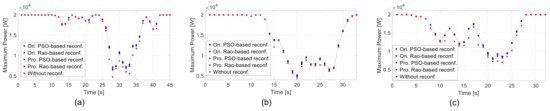
Figure 21.
Comparison of maximum output power profiles of TCT-configured, original-PSO-reconfigured, original-Rao-reconfigured, proposed-PSO-reconfigured, and proposed-Rao-reconfigured PV arrays under three shading cases without lagged time. (a) Case 1. (b) Case 2. (c) Case 3.
The performance metrics of the PV array are presented in Table 3. In Case 1 and Case 3, the proposed-PSO-reconfigured PV array has higher output power (P), higher PE, and suffer lower PL than the original-PSO-reconfigured PV array has. In Case 2, the original-PSO-reconfigured PV array has better performance metrics than the proposed-PSO-reconfigured PV array has. The proposed-Rao-reconfigured PV array has better output power, PE, and PL in Case 1 and Case 2 than the original-Rao-reconfigured PV array has. In Case 3, the performance metrics of the original-Rao-reconfigured PV array are better than that of the proposed-Rao-reconfigured PV array.
Table 3.
Summary performance metrics of PV array under PSC without considering time lagging.
Table 4 indicates the total number of switching times of the PV array with the original and proposed DPVAR models. In general, the proposed DPVAR models require fewer switching times than the original DPVAR models under the three studied MC patterns. This improvement comes from two factors. The first reason is the result of the power-optimized RA of the proposed DPVAR. Since the SDI of the proposed DPVAR less exceeds its activated threshold than the original DPVAR does, the proposed DPVAR requires fewer reconfiguration times. The second reason is the result of the proposed switching optimization.
Table 4.
Summary total number of switching times of PV array without time lagging.
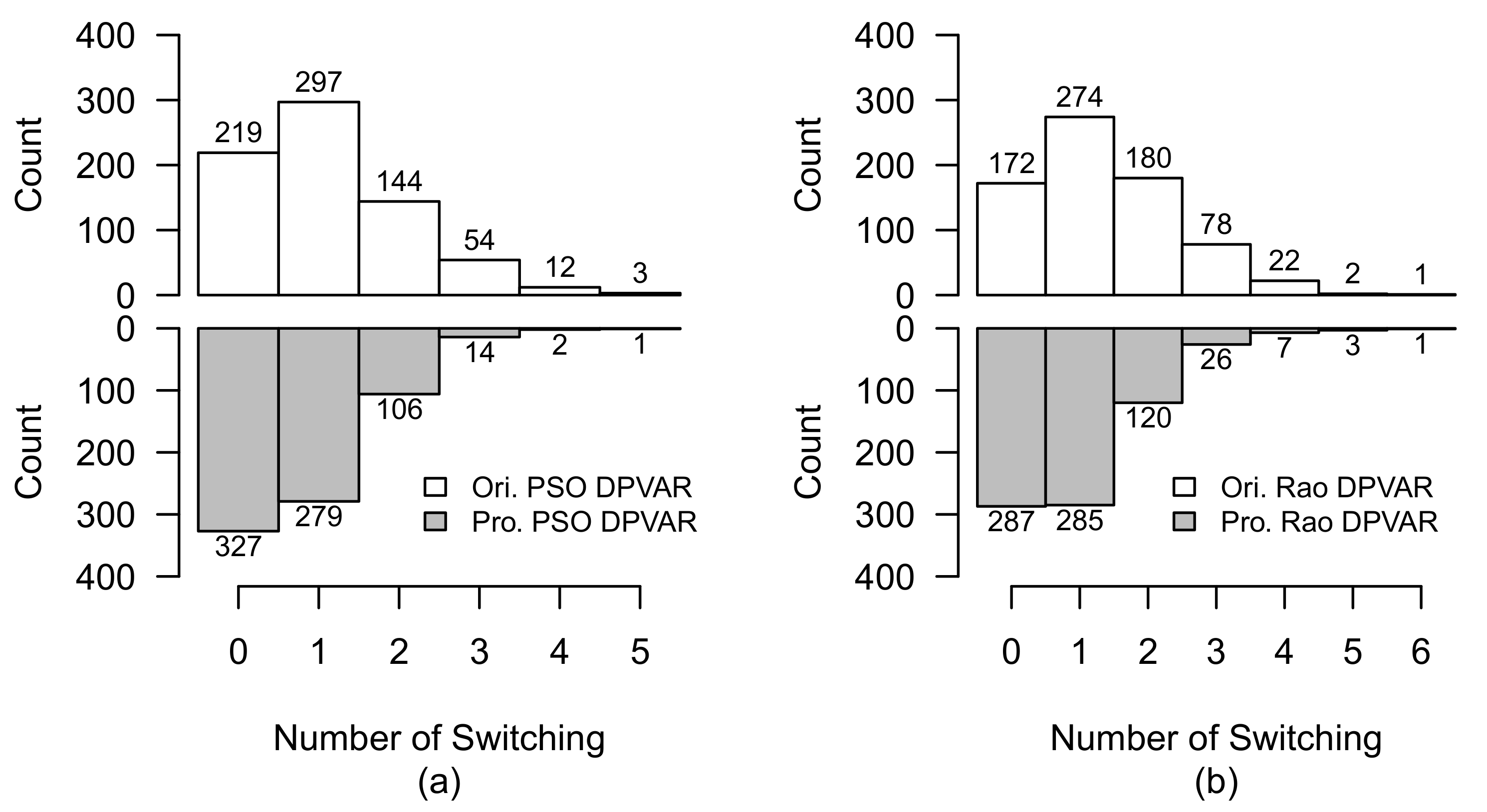
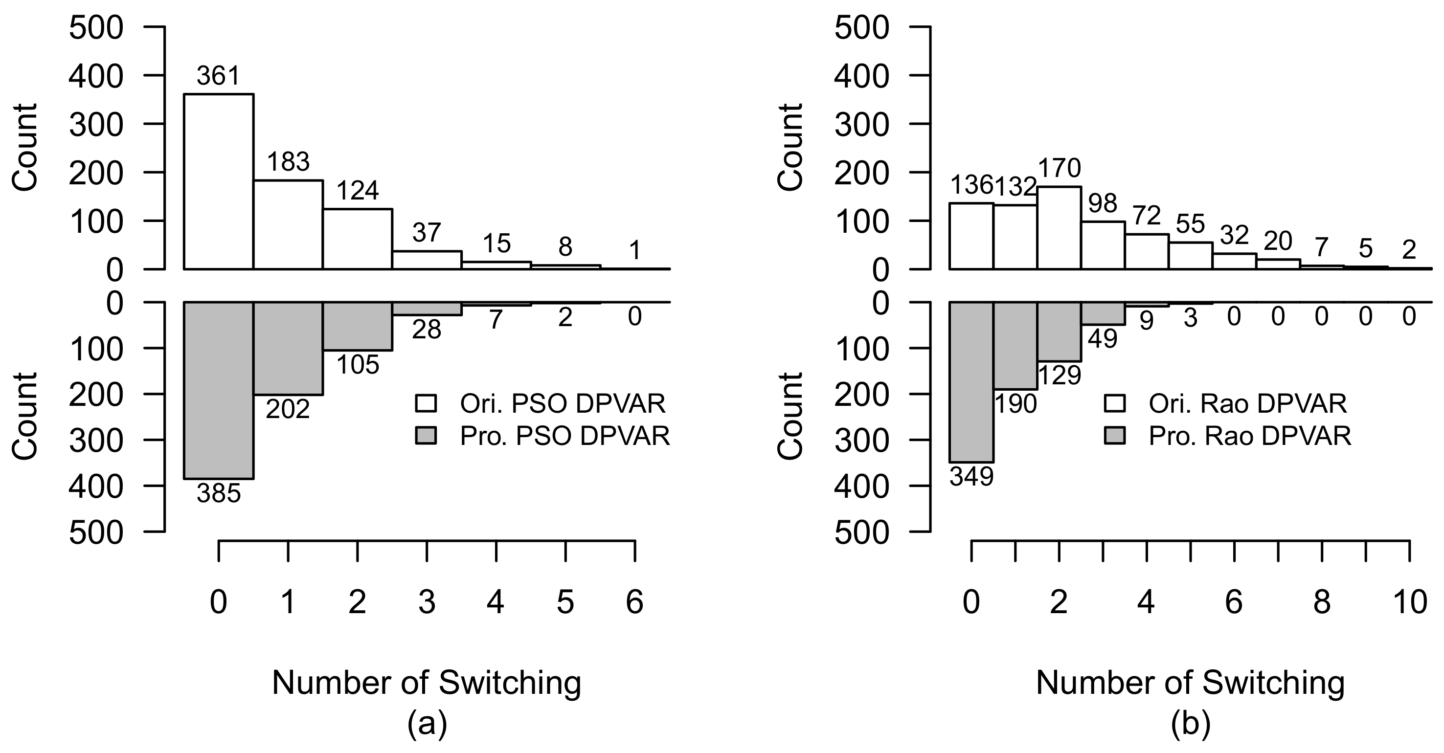
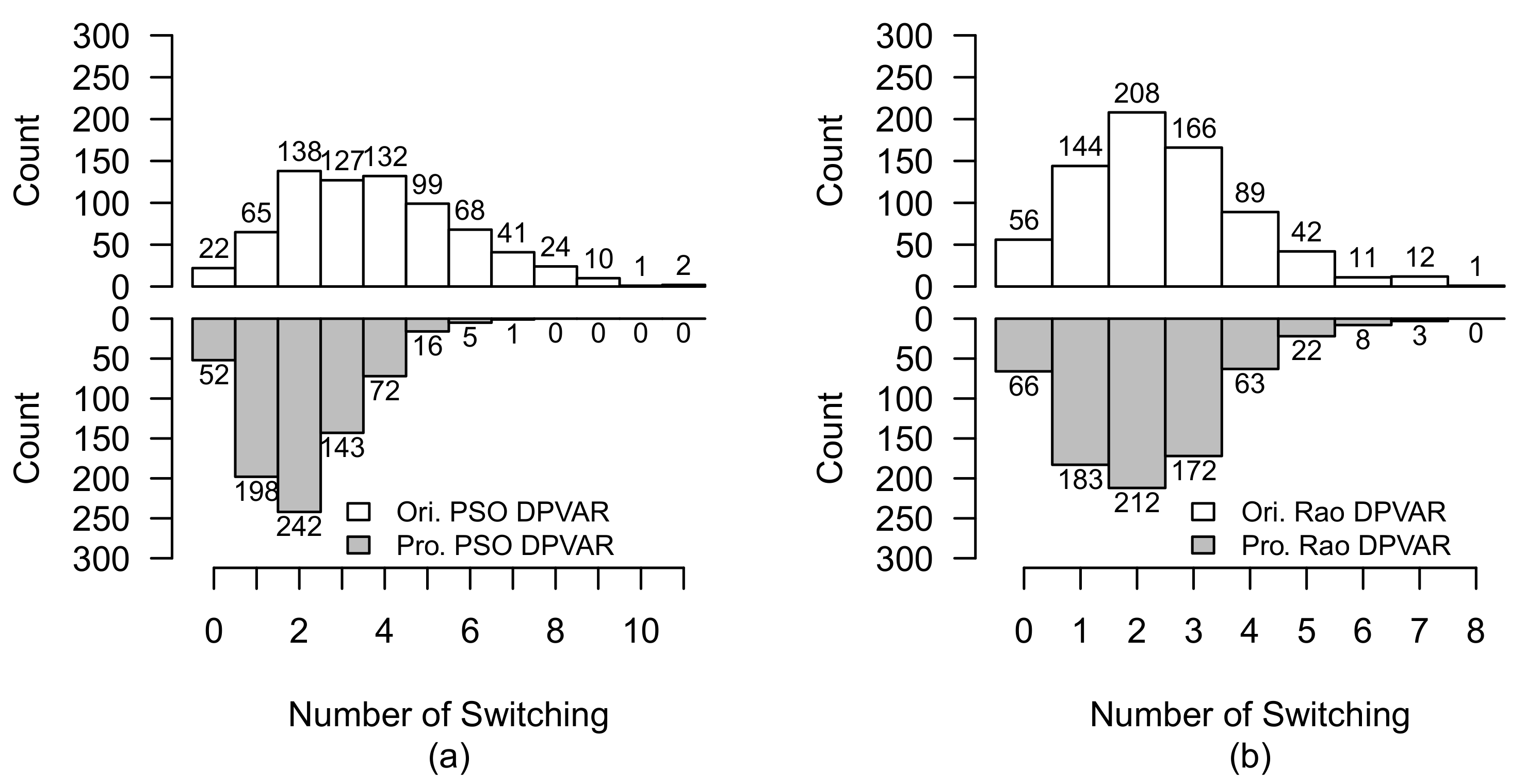
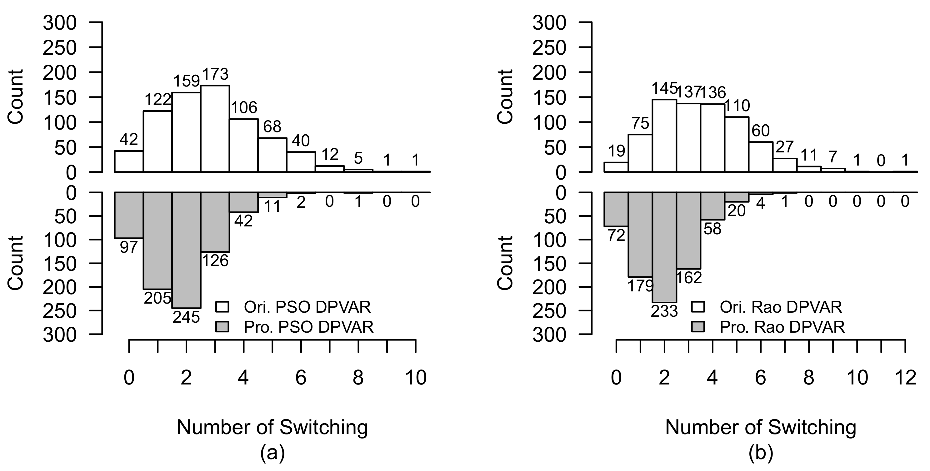
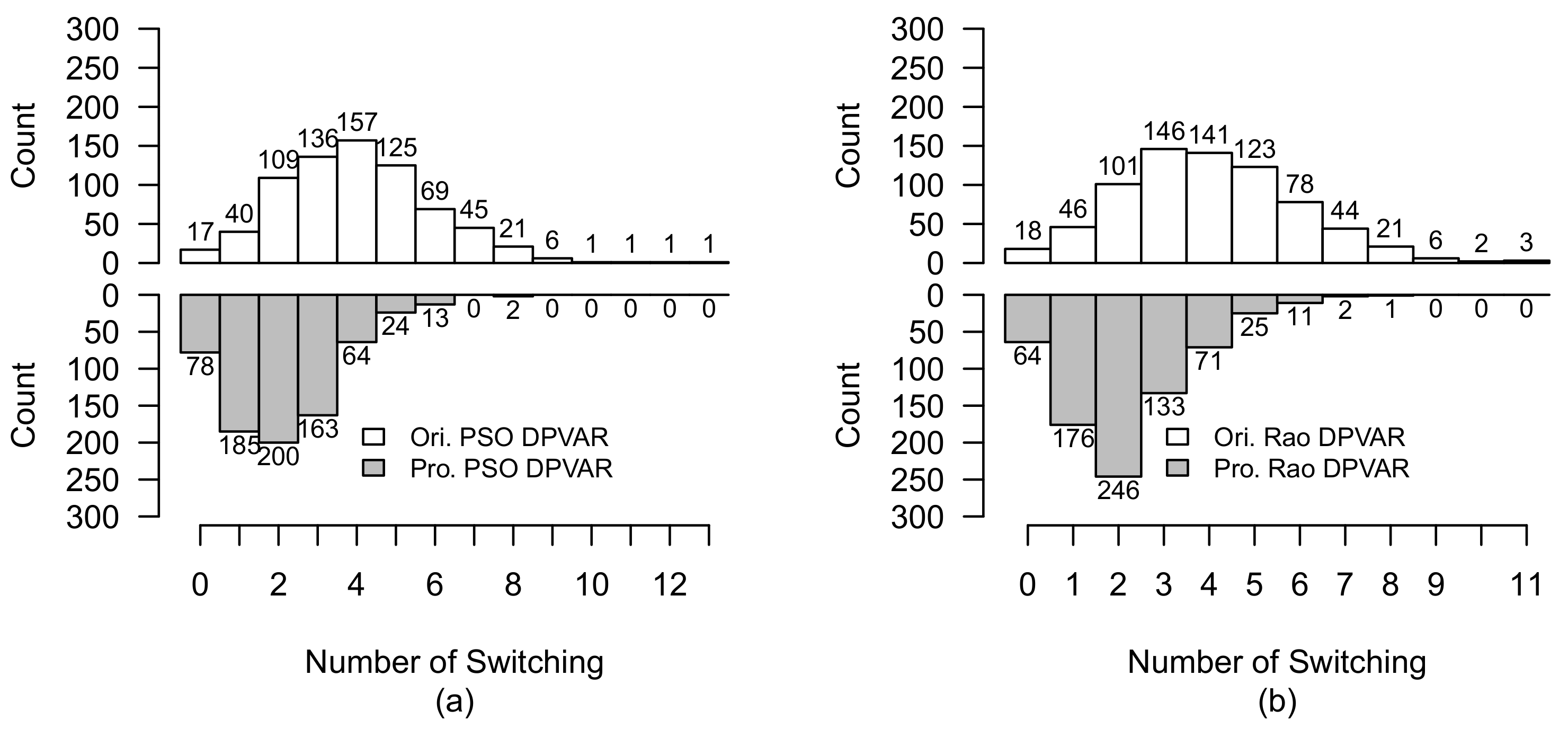
To validate the efficiency of the proposed switching optimization in terms of equally distributing the switching operation, Figure 22, Figure 23 and Figure 24 show the number of switches by the number of switching of the original and proposed DPVAR models under three MC patterns. In Figure 22, the number of switches that have more than one operation is reduced significantly after applying the proposed switching optimization. Whilst, the number of switches that have zero to one switching times are higher after applying the proposed switching optimization. For the proposed-Rao-reconfigured PV array, the switching optimization also allocates fewer switching times to the switches that have more than one time of switching operation. In the same token, the PV array with the proposed switching optimization in Case 2 and Case 3 all distribute fewer switching times on the active switches (Figure 23 and Figure 24). Especially, the original-Rao-reconfigured PV array in Case 3 (Figure 24b) has 32 switches with the six-time operation, 20 switches with the seven-time operation, 7 switches with the eight-time operation, 5 switches with the nine-time operation, and 2 switches with the ten-time operation. The number of these highly active switches are reduced to zero when applying proposed-Rao-based DPVAR.
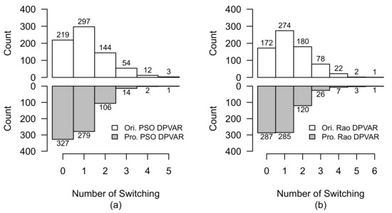
Figure 22.
Comparison of switching operation of original-reconfigured and proposed-reconfigured PV arrays under Case 1 without lagged time. (a) PSO-reconfigured PV array. (b) Rao-reconfigured PV array.
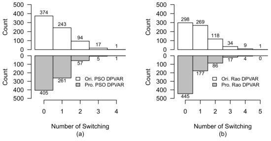
Figure 23.
Comparison of switching operation of original-reconfigured and proposed-reconfigured PV arrays under Case 2 without lagged time. (a) PSO-reconfigured PV array. (b) Rao-reconfigured PV array.

Figure 24.
Comparison of switching operation of original-reconfigured and proposed-reconfigured PV arrays under Case 3 without lagged time. (a) PSO-reconfigured PV array. (b) Rao-reconfigured PV array.
4.2.2. DPVAR with Time Lagging
Figure 25 shows the SDI on the PV array without the DPVAR and with the original and proposed DPVAR. The SDI of the proposed DPVAR is more fluctuated than that of the original DPVAR. In this case, the SDI exceeds its activated threshold many times. This can be explained that the obtained configurations do not correspond to the irradiance at that current time. This mismatch is caused by the time lag of the physical reconfiguration deployment. Figure 26 shows the maximum output power of the PV array under the continuous operation of the DPVAR considering time lagging. The proposed DPVAR models all perform better than the original DPVAR models do under three shading cases.
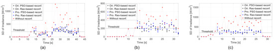
Figure 25.
Comparison of SDI of TCT-configured, original-PSO-reconfigured, original-Rao-reconfigured, proposed-PSO-reconfigured, and proposed-Rao-reconfigured PV arrays under three shading cases with lagged time. (a) Case 1. (b) Case 2. (c) Case 3.
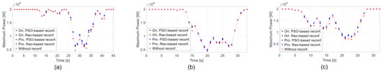
Figure 26.
Comparison of maximum output power profiles of TCT-configured, original-PSO-reconfigured, original-Rao-reconfigured, proposed-PSO-reconfigured, and proposed-Rao-reconfigured PV arrays under three shading cases with lagged time. (a) Case 1. (b) Case 2. (c) Case 3.
Table 5 demonstrates that the proposed-PSO-reconfigured and the proposed-Rao-reconfigured PV arrays have higher output power, higher PE, and lower PL compared to the original-PSO-reconfigured and proposed-Rao-reconfigured PV arrays. It is noteworthy that the original and proposed DPVAR models in the case with time lagging have lower output power, lower PE, and higher PL than the ones in the case without time lagging although the SDI is set lower than that in the case without time lagging. The reason also comes from the mismatch between the current configuration, which is obtained from the previous irradiance, with the current irradiance.
Table 5.
Summary performance metrics of PV array under PSC with time lagging.
Table 6 shows the total number of switching times of the PV array with the original and proposed DPVAR under all three MC patterns when considering time lagging. In general, the total number of switching times of the proposed DPVAR is reduced substantially than that of the original DPVAR. Especially, under Case 3, the number of switching is reduced almost twofold on the proposed-PSO-reconfigured PV array and the proposed-Rao-reconfigured PV array. However, the number of switching when considering time lagging is far larger than that without considering time lagging. The first reason is that the mismatch between the considered irradiance and the configuration of the PV array keeps SDI higher than its activated threshold many times. The second reason is that the SDI is set lower, in this case, to trade-off for the power improvement.
Table 6.
Summary total number of switching times of PV array with time lagging.
To evaluate the distribution of switching, Figure 27, Figure 28 and Figure 29 show the number of switches by the number of switching of the original and proposed DPVAR in three MC patterns. It is clear that the number of switching on highly active switches when considering time lagging also increases. In Case 1 of the MC (Figure 27), the PV array with the proposed-PSO DPVAR has a lower number of active switches (more than one time of switching) than the original-DPVAR-reconfigured PV array has. For the proposed-PSO-based DPVAR, there is no switch that has more than seven times the operation. Whilst, the proposed-PSO DPVAR has a higher number of switches that have zero to one switching times than the original-PSO DPVAR has. For the proposed-Rao-reconfigured PV array, the switching optimization also allocates fewer switching times on the switches that have more than one switching time. In the same token, the PV array with the proposed DPVAR in Case 2 (Figure 28) and Case 3 (Figure 29) all distribute fewer switching times on the active switches. In Case 2, the proposed-PSO-based DPVAR has only one switch with seven switching times. The proposed-Rao-based DPVAR has no switches that have more than seven operation times. In Case 3, the proposed-PSO-based DPVAR and the proposed-Rao-based DPVAR have no switch with more than eight switching times.

Figure 27.
Comparison of switching operation of original-reconfigured and proposed-reconfigured PV arrays under Case 1 with lagged time. (a) PSO-reconfigured PV array. (b) Rao-reconfigured PV array.

Figure 28.
Comparison of switching operation of original-reconfigured and proposed-reconfigured PV arrays under Case 2 with lagged time. (a) PSO-reconfigured PV array. (b) Rao-reconfigured PV array.
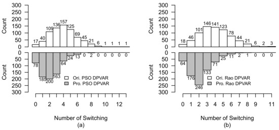
Figure 29.
Comparison of switching operation of original-reconfigured and proposed-reconfigured PV arrays under Case 3 with lagged time. (a) PSO-reconfigured PV array. (b) Rao-reconfigured PV array.
5. Conclusions
PSC, especially MC, substantially affects the operation of PV systems. To mitigate the effects of the PSC on the PV array, DPVAR is developed to minimize mismatch power losses and smooth the P-V characteristic of the PV array under PSC. This paper addresses the continuous operation of the DPVAR by emulating the direction, speed, shape, and thickness of the MC. The meta-heuristic-based RA can adapt to the practical moving clouds because the shading patterns are variable during their passing time. The superior performance of the proposed algorithms compared to the original algorithms has been proven under three shading patterns with heterogeneous shapes, sizes, and thickness. Under continuous operation, the efficacy of the proposed RA depends on the variability of the MC and has the most significant improvement under the cloud that moves across or vertically on the PV array. As a result, the output power improvement and power loss minimization are most clearly seen under, across, or vertically MC. This study also investigates the effects of time lagging on the continuous operation of the DPVAR. The time lagging engenders the mismatch between the obtained configuration and the irradiance of the PV array. This unintended phenomenon not only reduces the power enhancement, but also increases the switching operation of the DPVAR. Therefore, it is paramount to pre-process the RA before the PSC, especially for fast-happening PSCs such as the cloud. Finally, this study proposes a switching optimization to decrease the total number of switching actions and switching frequency on the highly active switches. However, as the number of switching is still high and the commercial switches are stressful because of continuous work as well, it is indispensable for future studies to work on structuring the switching board to reduce the number of required switches. In future related works, some experimental analyses need to be conducted to validate the ability of the DPVAR approaches in practice.
Author Contributions
T.N.-D.: Conceptualization, methodology, resources, project administration, supervision, funding acquisition, writing—reviewing and editing. D.N.-D.: methodology, formal analysis, software, writing—original draft preparation, data curation, visualization, investigation. T.L.-V.: conceptualization, methodology, formal analysis, software, writing—original draft preparation, data curation, visualization, investigation. G.F.: supervision, writing—reviewing and editing. All authors have read and agreed to the published version of the manuscript.
Funding
This research is funded by the Hanoi University of Science and Technology (HUST) under project number T2020-SAHEP-005.
Data Availability Statement
Data sharing not applicable.
Conflicts of Interest
The authors declare no conflict of interest.
References
- Rodrigo, P.M.; Talavera, D.L.; Fernández, E.F.; Almonacid, F.M.; Pérez-Higueras, P.J. Optimum capacity of the inverters in concentrator photovoltaic power plants with emphasis on shading impact. Energy 2019, 187, 115964. [Google Scholar] [CrossRef]
- Murtaza, A.F.; Sher, H.A.; Al-Haddad, K.; Spertino, F. Module Level Electronic Circuit Based PV Array for Identification and Reconfiguration of Bypass Modules. IEEE Trans. Energy Convers. 2021, 36, 380–389. [Google Scholar] [CrossRef]
- Karmakar, B.K.; Karmakar, G. A Current Supported PV Array Reconfiguration Technique to Mitigate Partial Shading. IEEE Trans. Sustain. Energy 2021, 12, 1449–1460. [Google Scholar] [CrossRef]
- Rani, B.I.; Ilango, G.S.; Nagamani, C. Enhanced power generation from PV array under partial shading conditions by shade dispersion using Su Do Ku configuration. IEEE Trans. Sustain. Energy 2013, 4, 594–601. [Google Scholar] [CrossRef]
- Potnuru, S.R.; Pattabiraman, D.; Ganesan, S.I.; Chilakapati, N. Positioning of PV panels for reduction in line losses and mismatch losses in PV array. Renew. Energy 2015, 78, 264–275. [Google Scholar] [CrossRef]
- Sai Krishna, G.; Moger, T. Optimal SuDoKu Reconfiguration Technique for Total-Cross-Tied PV Array to Increase Power Output under Non-Uniform Irradiance. IEEE Trans. Energy Convers. 2019, 34, 1973–1984. [Google Scholar] [CrossRef]
- Yadav, K.; Kumar, B.; Swaroop, D. Mitigation of Mismatch Power Losses of PV Array under Partial Shading Condition using novel Odd Even Configuration. Energy Rep. 2020, 6, 427–437. [Google Scholar] [CrossRef]
- Nguyen, D.; Lehman, B. An adaptive solar photovoltaic array using model-based reconfiguration algorithm. IEEE Trans. Ind. Electron. 2008, 55, 2644–2654. [Google Scholar] [CrossRef]
- Velasco-Quesada, G.; Guinjoan-Gispert, F.; Piqué-López, R.; Román-Lumbreras, M.; Conesa-Roca, A. Electrical PV array reconfiguration strategy for energy extraction improvement in grid-connected PV systems. IEEE Trans. Ind. Electron. 2009, 56, 4319–4331. [Google Scholar] [CrossRef]
- Sanseverino, E.R.; Ngoc, T.N.; Cardinale, M.; Li Vigni, V.; Musso, D.; Romano, P.; Viola, F. Dynamic programming and Munkres algorithm for optimal photovoltaic arrays reconfiguration. Sol. Energy 2015, 122, 347–358. [Google Scholar] [CrossRef]
- Ngo Ngoc, T.; Phung, Q.N.; Tung, L.N.; Riva Sanseverino, E.; Romano, P.; Viola, F. Increasing efficiency of photovoltaic systems under non-homogeneous solar irradiation using improved Dynamic Programming methods. Sol. Energy 2017, 150, 325–334. [Google Scholar] [CrossRef]
- Ngoc, T.N.; Sanseverino, E.R.; Quang, N.N.; Romano, P.; Viola, F.; Van, B.D.; Huy, H.N.; Trong, T.T.; Phung, Q.N. A hierarchical architecture for increasing efficiency of large photovoltaic plants under non-homogeneous solar irradiation. Sol. Energy 2019, 188, 1306–1319. [Google Scholar] [CrossRef]
- Bonthagorla, P.K.; Mikkili, S. A Novel Fixed PV Array Configuration for Harvesting Maximum Power from Shaded Modules by Reducing the Number of Cross-Ties. IEEE J. Emerg. Sel. Top. Power Electron. 2021, 9, 2109–2121. [Google Scholar] [CrossRef]
- Babu, T.S.; Yousri, D.; Balasubramanian, K. Photovoltaic Array Reconfiguration System for Maximizing the Harvested Power Using Population-Based Algorithms. IEEE Access 2020, 8, 109608–109624. [Google Scholar] [CrossRef]
- Muhammad Ajmal, A.; Ramachandaramurthy, V.K.; Naderipour, A.; Ekanayake, J.B. Comparative analysis of two-step GA-based PV array reconfiguration technique and other reconfiguration techniques. Energy Convers. Manag. 2021, 230, 113806. [Google Scholar] [CrossRef]
- Zhang, X.; Li, C.; Li, Z.; Yin, X.; Yang, B.; Gan, L.; Yu, T. Optimal mileage-based PV array reconfiguration using swarm reinforcement learning. Energy Convers. Manag. 2021, 232, 113892. [Google Scholar] [CrossRef]
- Rajan, N.A.; Shrikant, K.D.; Dhanalakshmi, B.; Rajasekar, N. Solar PV array reconfiguration using the concept of Standard deviation and Genetic Algorithm. Energy Procedia 2017, 117, 1062–1069. [Google Scholar] [CrossRef]
- Babu, T.S.; Ram, J.P.; Dragičević, T.; Miyatake, M.; Blaabjerg, F.; Rajasekar, N. Particle swarm optimization based solar PV array reconfiguration of the maximum power extraction under partial shading conditions. IEEE Trans. Sustain. Energy 2018, 9, 74–85. [Google Scholar] [CrossRef]
- Fathy, A. Recent meta-heuristic grasshopper optimization algorithm for optimal reconfiguration of partially shaded PV array. Sol. Energy 2018, 171, 638–651. [Google Scholar] [CrossRef]
- Fathy, A.; Rezk, H.; Yousri, D. A robust global MPPT to mitigate partial shading of triple-junction solar cell-based system using manta ray foraging optimization algorithm. Sol. Energy 2020, 207, 305–316. [Google Scholar] [CrossRef]
- Romano, P.; Candela, R.; Cardinale, M.; Li Vigni, V.; Musso, D.; Riva Sanseverino, E. Optimization of photovoltaic energy production through an efficient switching matrix. J. Sustain. Dev. Energy Water Environ. Syst. 2013, 1, 227–236. [Google Scholar] [CrossRef]
- Chen, X.; Du, Y.; Lim, E.; Wen, H.; Yan, K.; Kirtley, J. Power ramp-rates of utility-scale PV systems under passing clouds: Module-level emulation with cloud shadow modeling. Appl. Energy 2020, 268, 114980. [Google Scholar] [CrossRef]
- Nguyen-Duc, T.; Nguyen-Duc, H.; Le-Viet, T.; Takano, H. Single-diode models of PV modules: A comparison of conventional approaches and proposal of a novel model. Energies 2020, 13, 1296. [Google Scholar] [CrossRef]
- Nguyen, T.D.; Le, T.V.; Fujita, G. Identification of photovoltaic-generation-characteristic at real-time conditions by improved single-diode model. IET Renew. Power Gener. 2022, 16, 223–236. [Google Scholar] [CrossRef]
- Villalva, M.G.; Gazoli, J.R.; Ruppert Filho, E. Comprehensive Approach to Modeling and Simulation of Photovoltaic Arrays. Sol. Energy 2009, 84, 1244–1254. [Google Scholar] [CrossRef]
- Lo Brano, V.; Orioli, A.; Ciulla, G.; Di Gangi, A. An improved five-parameter model for photovoltaic modules. Sol. Energy Mater. Sol. Cells 2010, 94, 1358–1370. [Google Scholar] [CrossRef]
- Jazayeri, M.; Jazayeri, K.; Uysal, S. Adaptive photovoltaic array reconfiguration based on real cloud patterns to mitigate effects of non-uniform spatial irradiance profiles. Sol. Energy 2017, 155, 506–516. [Google Scholar] [CrossRef]
- Kennedy, J.; Eberhart, R. Particle swarm optimization. In Proceedings of the ICNN’95—International Conference on Neural Networks, Perth, Australia, 27 November–1 December 1995; Volume 4, pp. 1942–1948. [Google Scholar] [CrossRef]
- Rao, R.V. Rao algorithms: Three metaphor-less simple algorithms for solving optimization problems. Int. J. Ind. Eng. Comput. 2020, 11, 107–130. [Google Scholar] [CrossRef]
- BISOL BSU 227-245 Wp Multicrystalline Silicon Roof Integrated PV Modules. Available online: https://pdf.archiexpo.com/pdf/bisol/bsu227-245/66976-93655.html (accessed on 22 March 2022).


Publisher’s Note: MDPI stays neutral with regard to jurisdictional claims in published maps and institutional affiliations. |
© 2022 by the authors. Licensee MDPI, Basel, Switzerland. This article is an open access article distributed under the terms and conditions of the Creative Commons Attribution (CC BY) license (https://creativecommons.org/licenses/by/4.0/).