Article

A Critical Analysis of Modeling Aspects of D-STATCOMs for Optimal Reactive Power Compensation in Power Distribution Networks

by
Subrat Kumar Dash
1,
Sivkumar Mishra
2,* and
Almoataz Y. Abdelaziz
3,*
1
Department of Electrical Engineering, Government College of Engineering, Kalahandi (GCEK), Bhawanipatna 766002, Odisha, India
2
Department of Electrical Engineering, Centre for Advanced Post Graduate Studies, BPUT Rourkela (CAPGS, BPUT), Rourkela 769015, Odisha, India
3
Faculty of Engineering and Technology, Future University in Egypt, Cairo 11835, Egypt
*
Authors to whom correspondence should be addressed.
Energies 2022, 15(19), 6908; https://doi.org/10.3390/en15196908
Submission received: 16 August 2022 / Revised: 15 September 2022 / Accepted: 19 September 2022 / Published: 21 September 2022

Abstract

:
Distribution static compensators (D-STATCOMs) can enhance the technical performance of the power distribution network by providing rapid and continuous reactive power support to the connected bus. Accurate modeling and efficient utilization of D-STATCOMs can maximize their utility. In this regard, this article offers a novel current-injection-based D-STATCOM model under the power control mode of operation for the reactive power compensation of the power distribution network. The versatility of the proposed D-STATCOM model is demonstrated by combining it with two of the most established distribution load flow techniques, viz., the forward–backward sweep load flow and the BIBC–BCBV-matrix-based direct load flow. Further, the allocation of the proposed D-STATCOM model is carried out under a multiobjective mathematical formulation consisting of various technical and economic indices such as the active power loss reduction index, voltage variation minimization index, voltage stability improvement index and annual expenditure index. A novel parameter-free metaheuristic algorithm, namely a student-psychology-based optimization algorithm, is proposed to determine the optimal assignment of the different number of D-STATCOM units under the multiobjective framework. The proposed allocation scheme is implemented on a standard 33-bus test system and on a practical 51-bus rural distribution feeder. The obtained results demonstrate that the proposed D-STATCOM model can be efficiently integrated into the distribution load flow algorithms. The student-psychology-based optimization algorithm is found to be robust and efficient in solving the optimal allocation of D-STATCOMs as it yields minimum power loss compared to other established approaches for 33-bus PDNs. Further, the economic analysis carried out in this work can guide network operators in deciding on the number of D-STATCOMs to be augmented depending on the investment costs and the resulting savings.

Graphical Abstract

1. Introduction

In a deregulated power system structure, high-quality power supply plays a vital role for power distribution network operators (PDNOs). However, the radial mode of functioning of the traditional passive distribution grid leads to poor system performance. Further, with load expansion on the rise, PDNOs need to envisage optimal planning of the power distribution network (PDN) considering the augmentation of state-of-the-art devices to foster dependable and quality power for the end users. Various power quality (PQ) issues such as voltage sag, voltage swell, flicker, voltage interruption, harmonic distortions and many others have a profound impact on the customers in terms of data loss, increased production downtime, shutdown of critical loads and recurring equipment failures resulting in significant economic loss [1]. Optimal reactive power management can alleviate the majority of the PQ issues, such as voltage sag, voltage swell and interruption [2]. Traditionally, a combination of fixed and switched shunt capacitor banks (SCBs) is optimally allocated to manage the reactive power across the PDN. However, from operational aspects, capacitors connected along with inductive elements may cause oscillatory response, and more importantly, they cannot deliver continuously varying reactive power [3]. On the other hand, synchronous condensers (SCs) can inject the required varying reactive power into the connected bus. However, SCs are very expensive and need frequent maintenance [4].
Amidst the issues with traditional strategies (SCBs/SCs) to optimally manage the reactive power of the PDN, custom power devices (CPDs) are becoming more promising alternatives for PDNOs. Custom power devices [5] are static controllers used in medium-voltage distribution systems (1–38 kV) to mitigate power quality concerns related to RMS voltage variations [6]. Different CPDs such as a series-connected dynamic voltage restorer (DVR) can alleviate voltage sag or other voltage imbalances, a shunt-connected distribution static compensator (D-STATCOM) can mitigate current-related PQ issues, and a unified power quality conditioner (UPQC) with both series and shunt arms is effective in minimizing both voltage- and current-related PQ disturbances. A D-STATCOM, more specifically, is effective in suppressing current-related issues such as reactive power compensation [7], voltage regulation [8], current harmonics and load balancing [9]. Moreover, D-STATCOMs cost less, have a compact size, inject minimal harmonics and require simple control algorithms compared to other CPD variants [7].
An accurate modeling of the D-STATCOM can ensure both correct incorporation and effective utilization of the device. Different D-STATCOM modeling approaches are available in the literature. Most of the earlier approaches consider the distribution system as a single source connected to a single sensitive load for deriving the D-STATCOM model [8] which can only be helpful for accessing the dynamic impact of the device. However, from a planning perspective, the model of a PDN connected to several load centers is required to study the steady-state performance. The steady-state model of the D-STATCOM (SMD) was derived as a synchronous condenser [10] and a static compensator (STATCOM) [11,12,13]. An accurate D-STATCOM model (ADM) was curated in [8] for boosting the steady-state voltage of the sensitive bus (SB) to 1.0 p.u. In this approach, the voltage phase angle of the SB and the magnitude of the current injected by the D-STATCOM were the unknowns that were computed by integrating the D-STATCOM model into a forward–backward sweep load flow (FBS-LF). Likewise, the authors of [14] modeled a D-STATCOM to maintain the SB voltage at 1.0 p.u. The voltage phase angle of the SB and the current injected by the D-STATCOM were calculated from the load flow and were further utilized to determine the capacity of the D-STATCOM. In [15], the authors incorporated the ADM into a BIBC–BCBV-matrix-based direct load flow (BB-DLF). The authors in [16] suggested a D-STATCOM with an optimal phase angle for reactive power regulation. The size of the D-STATCOM was obtained by inserting the optimal phase angle at the connected bus. The derived model was linked with a forward–backward sweep load flow procedure. For an unbalanced PDN, a three-phase SDM was presented in [17]. For the relatively unbalanced secondary distribution system, a three-phase D-STATCOM model is suitable. However, for primary distribution networks, D-STATCOM’s single-phase modeling is employed. An SDM for mesh distribution networks (MPDNs) was introduced in [18] by utilizing a BB-DLF.
Several D-STATCOM allocation strategies were discussed in the earlier literature. Few researchers have used sensitivity-based techniques to first identify the suitable location for the D-STATCOM followed by metaheuristic algorithms to determine the optimal device size [15,19,20,21]. However, the use of sensitivity approaches to pre-locate placements may not yield optimal allocation for D-STATCOMs [22]. Simultaneous optimal allocation of D-STATCOMs was also accomplished exclusively using different metaheuristic techniques in [23,24,25,26]. However, metaheuristic approaches with algorithm-specific control parameters introduce additional complexity to the optimal allocation of D-STATCOMs (OADS) [27].
The above discussion highlights that steady-state D-STATCOM models can be more effective to access the long-term impact of the allocation of the device on the entire PDN. In the earlier models [8,14,15,16], the size of the D-STATCOM is determined from the results of the distribution load flow. OADS using parametric metaheuristic approaches is quite complex. This motivated the authors to present a novel current-injection-based steady-state D-STATCOM model that can effortlessly integrate with distribution load flows where the size of the device is not dependent on the load flow results. Further, a parameter-free metaheuristic technique, namely student-psychology-based optimization (SPBO), is suggested to solve OADS considering a multiobjective formulation consisting of technical and economic indices. Student-psychology-based optimization [28] is a new metaheuristic technique that was inspired by the psychology of students belonging to different study groups to continuously improve their class performance to be the best student. The SPBO algorithm does not have any algorithm-specific parameters except trivial parameters such as initial population size and the maximum number of iterations. Due to this, the SPBO algorithm has been successfully implemented to solve various engineering optimization problems [29,30,31].
The rest of the manuscript is organized as follows: Section 2 revisits two earlier D-STATCOM models followed by the proposed current-injection-based D-STATCOM modeling. In Section 3, the detailed steps for integrating the proposed D-STATCOM model with an FBS-LF and a BB-DLF are discussed. Multiobjective problem formulation for the OADS and SPBO algorithm is introduced in Section 4. OADS using SPBO is proposed in Section 5. The detailed result analysis is carried out in Section 6. Conclusion of the work is summarized in Section 7.

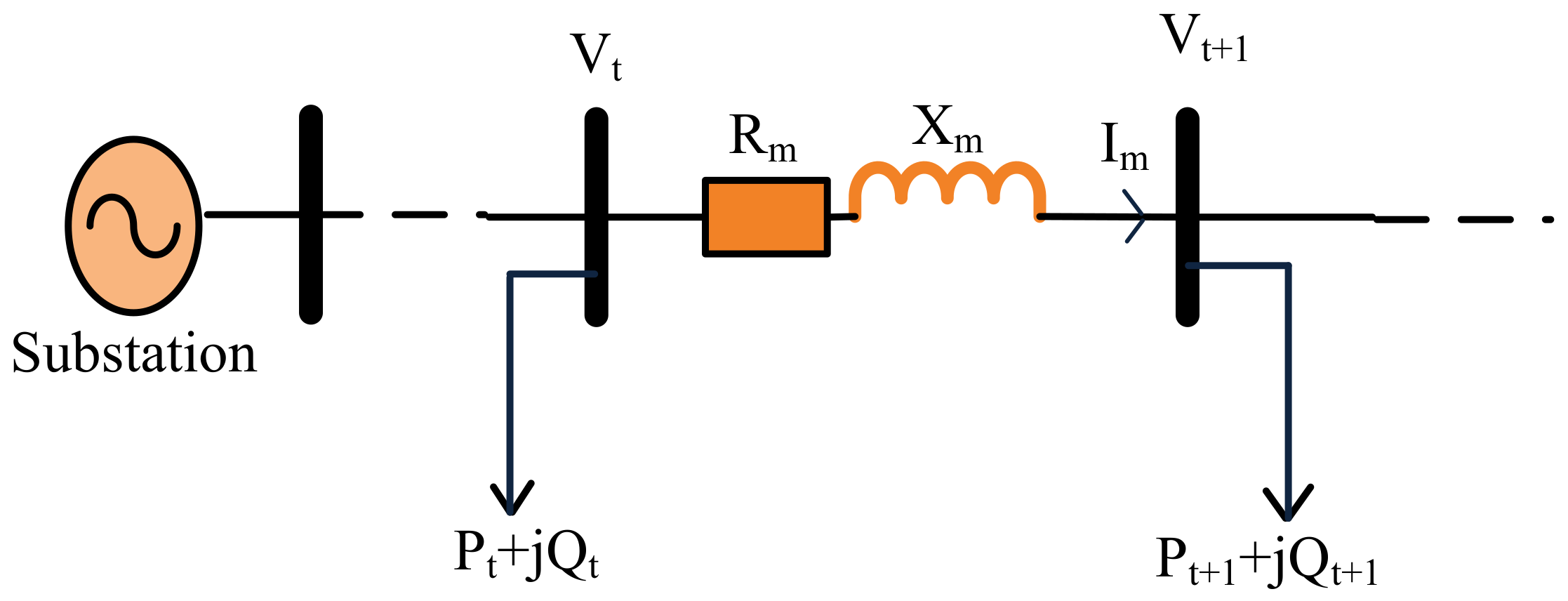
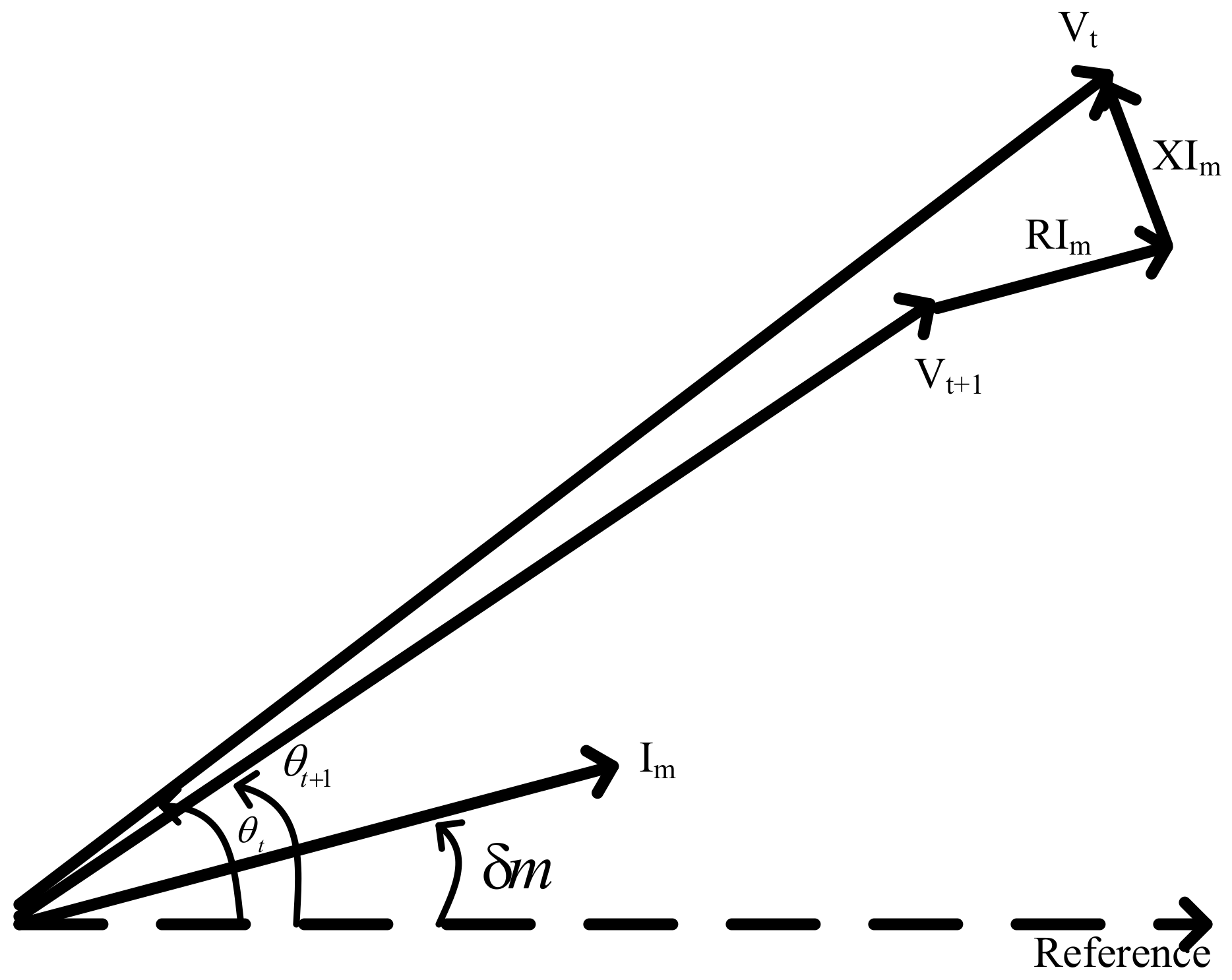
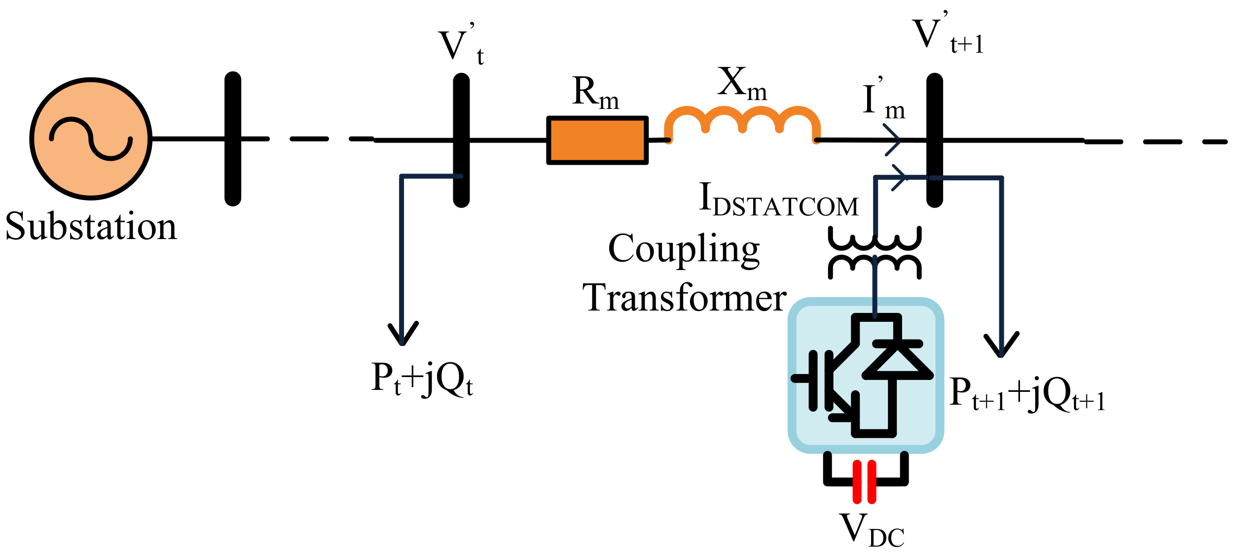
2. D-STATCOM Modeling Features

The D-STATCOM is a shunt-connected CPD capable of exchanging both active and reactive power to improve the power quality at the distribution level. It includes an IGBT- or GTO-based voltage source converter (VSC), DC capacitor bus, energy storage device, coupling transformer and tuned filter. Because of the VSC’s ability to swap roles as generalized capacitive and inductive reactance synchronously, the D-STATCOM may export or import reactive power at the point of common coupling (PCC) to facilitate continuous reactive power compensation up to the device’s maximum MVA rating. The DC capacitor bus helps maintain a constant DC link voltage at the DC side of the device and thereby helps regulate the output AC voltage of the D-STATCOM. A D-STATCOM coupled with energy storage devices can deliver active power in addition to reactive power support. The AC side of the VSC is interfaced with the PCC through the coupling transformer. A tuned filter is designed to suppress the harmonics within the stipulated margin.
The D-STATCOM may operate either in power control mode (PCM) or voltage control mode (VCM) [12]. In PCM, a soft voltage constraint is applied at the compensated node (CN), and the size of the D-STATCOM is estimated to provide the necessary reactive power compensation at the PCC and also to the downstream nodes. So, the CN is represented as a PQ node. Meanwhile, in VCM, a harder voltage constraint is imposed on the CN to provide regulated voltage locally for the exigent customers (critical load), and therefore the size of the D-STATCOM is determined to provide steady-state voltage compensation at the CN. Thus, the CN is modeled as a PV node. A schematic representation of a D-STATCOM as a PQ bus and a PV bus is shown in Figure 1.
Let us consider a part of a PDN (consecutive two nodes) where the D-STATCOM is intended to be allocated. Figure 2 depicts the part of the PDN (consecutive two nodes) before the allocation of the D-STATCOM.
Applying Kirchhoff’s voltage law (KVL) to the part of the PDN shown in Figure 2 results in the following equation.
V t + 1 θ t + 1 = V t θ t ( R m + j X m ) I m δ m
where Vt and Vt+1 are the bus voltages of t and t + 1 node. θt and θt+1 are the corresponding phase angles, respectively. Im and δm represent the branch current and corresponding phase angle of the mth branch. Branch resistance and reactance of the mth branch are represented by Rm and Xm, respectively. Figure 3 depicts the phasor diagram corresponding to Equation (1).
Now let us connect a D-STATCOM to the t + 1 bus, and the compensated PDN of Figure 2 is now drawn in Figure 4. Hence, the modified KVL equation for the compensated PDN is obtained as:
V t + 1 θ t + 1 = V t θ t ( R m + j X m ) I m δ m + I D S T A T C O M ψ
where ID-STATCOM and ψ are the current injected and phase angle of the D-STATCOM, respectively. The phasor diagram corresponding to Equation (2) is shown in Figure 5.
From the phasor diagram, one can say that the voltage magnitude of the compensated bus has changed from Vt+1 to Vt+1’ due to the additional current supplied by the D-STATCOM.

2.1. Approach A1 [8]

In this approach, the D-STATCOM is modeled as a reactive power source. So, the current supplied by the D-STATCOM (IDSTACOM) will be in quadrature to the voltage of the compensated node (Vt+1′). Hence,
ψ = π 2 + θ t + 1
Now, substituting Equation (3) in Equation (2) and then separating real and imaginary parts, the following equations are generated.
V t + 1 cos θ t + 1 = e V t θ t + X m I D S T A T C O M sin π 2 + θ t + 1 e Z m I m δ m R m I D S T A T C O M cos π 2 + θ t + 1
V t + 1 sin θ t + 1 = m V t θ t X m I D S T A T C O M cos π 2 + θ t + 1 m Z m I m δ m R m I D S T A T C O M sin π 2 + θ t + 1
Let us define the following
a 1 = e V t θ t e Z m I m δ m ,
a 2 = m V t θ t m Z m I m δ m
a 3 = V t + 1
a 4 = R and
a 5 = X
Then,
I D S T A T C O M = a 3 cos θ t + 1 a 1 a 4 sin θ t + 1 a 5 cos θ t + 1
I D S T A T C O M = a 3 sin θ t + 1 a 2 a 5 sin θ t + 1 + a 4 cos θ t + 1
Now, equating Equations (6) and (7), we obtain,
a 1 a 5 a 2 a 4 sin θ t + 1 + a 1 a 4 a 2 a 5 cos θ t + 1 + a 3 a 4 = 0
Let k 1 = a 1 a 5 a 2 a 4 , k 2 = a 1 a 4 + a 2 a 5 and x = sin θ t + 1 .
Then,
k 1 2 + k 2 2 x 2 + 2 k 1 a 3 a 4 x + a 3 2 a 4 2 k 2 2 = 0
After finding the root of Equation (9), θ t + 1 can be determined as:
θ t + 1 = sin 1 x
As Equation (9) yields two roots, the correct root is identified by applying load flow conditions. Now, the current injected by the D-STATCOM can be computed using Equation (6) or Equation (7). The size of the D-STATCOM is given by:
j Q D S T A T C O M = V t + 1 θ t + 1 I D S T A T C O M * π 2 + θ t + 1
In this approach, the size of the D-STATCOM is computed from the load for ensuring the voltage of the CN is 1.0. Hence, this modeling technique is called VCM–SDM.

2.2. Approach A2 [7]

The authors, in this approach, derived an analytical modeling of the D-STATCOM based on optimal phase angle injection at the CN. The CN is treated as a PQ node, and therefore this modeling is called PCM–SDM. The model is suitably integrated with the FBS-LF. The detailed mathematical modeling is presented below.
The modified KVL equation after the integration of the D-STATCOM at t + 1 node and the phase angle of the current supplied by the D-STATCOM were already expressed in Equations (2) and (3). Now, applying some algebraic manipulation, the real and imaginary parts of IDSTACOM can be expressed as:
I D S T A T C O M cos ( θ t + 1 + π 2 ) = V t R m cos θ t R m 2 + X m 2 + V t X m sin θ t R m 2 + X m 2 V t + 1 R m cos θ t + 1 R m 2 + X m 2 V t + 1 X m sin θ t + 1 R m 2 + X m 2 I m cos δ m
I D S T A T C O M cos ( θ t + 1 + π 2 ) = V t R m sin θ t R m 2 + X m 2 V t X m cos θ t R m 2 + X m 2 V t + 1 R m sin θ t + 1 R m 2 + X m 2 + V t + 1 X m cos θ t + 1 R m 2 + X m 2 I m sin δ m
From Equations (12) and (13), the magnitude of the current injected by the D-STATCOM can be obtained as:
I D S T A T C O M = [ C 1 sin δ m θ t + φ ] [ C 2 sin δ m θ t + 1 + φ ] sin δ m ψ
where C 1 = V t R m 2 + X m 2 and C 2 = V t + 1 R m 2 + X m 2 .
Φ is a unique angle that satisfies the following conditions: 1. π < φ < π and 2. tan φ = X m R m .
This model of the D-STATCOM is integrated into the FBS-LF at the bus by modifying its reactive load demand as:
Q L o a d ( t ) = Q L o a d ( t ) Q D S T A T C O M
where the size of the D-SATACOM is obtained from Equation (11) for a specific value of θ t . So, in this modeling, the size of the D-STATCOM is a function of the phase angle of the CN. The optimal size of the D-STATCOM corresponds to the optimal location of the phase angle of the CN. Generally, in control applications of the D-STATCOM, phase-angle-based control has not been preferred as it produces both active and reactive power to regulate voltage at the CN.

2.3. Proposed PCM–D-STATCOM Modeling

In the proposed modeling approach, the D-STATCOM is considered as a current source (ID-STATCOM) whose magnitude and direction are decided by the relative polarity between the D-STATCOM output voltage (VD-STATCOM) and the voltage of the compensated node (VCN). If VD-STATCOM is greater than VCN, then ID-STATCOM flows from the D-STATCOM to the PCC, and if VCN is greater than VD-STATCOM, then ID-STATCOM will flow in the opposite direction.
In general, the power flow equation of the D-STATCOM coupled with energy-storing devices can be written as:
S D S T A T C O M = P D S T A T C O M j Q D S T A T C O M = V t + 1 V D S T A T C O M X L sin α V t + 1 V D S T A T C O M X L cos α V t + 1 2 X L
where SD-STATCOM, PD-STATCOM and QD-STATCOM are the apparent power, real power and reactive power of the D-STATCOM, respectively. VD-STATCOM is the output AC phase voltage of the D-STATCOM, and XL is the leakage reactance. α represents the relative phase angle difference between Vt+1′ and VD-STATCOM.
In the present work, the D-STACOM is considered to be capable of exchanging reactive power only. So, PD-STATCOM = 0, and correspondingly, from Equation (16), α = 0. It implies that for the D-STACOM to exchange reactive power only, the voltages of the compensated node (Vt+1′) and the D-STACOM (VD-STATCOM) should in the same phase. Hence,
V D S T A T C O M = V t + 1 = θ t + 1
Further, the DC bus voltage decides the magnitude of the output AC phase voltage of the D-STATCOM (VD-STATCOM) which is often regulated by the D-STATCOM control algorithm. Without the loss of any generality, in the present study, the voltage magnitude of the D-STATCOM voltage is considered as 1.0 p.u. Hence, it is the difference between the output AC phase voltage of the D-STATCOM and the voltages of the compensated node (Vt+1′) (and the leakage reactance connecting the two voltage sources) that will decide the magnitude and direction of the current injected by the D-STATCOM at the PCC. Therefore, the size of the D-STATCOM can be determined using Equation (11). Now, the expression for IDSTACOM in terms of QD-STATCOM and VD-STATCOM is obtained as:
I D S T A T C O M = j Q D S T A T C O M V D S T A T C O M * = Q D S T A T C O M V D S T A T C O M θ t + 1 + π 2
In Equation (18), the value of θt+1′ is unknown. To compute it, Equation (18) is first substituted in Equation (2), and then applying a few algebraic manipulations, the real and imaginary parts of modified Equation (2) are formed which are:
Real part:
V t + 1 cos θ t + 1 = e [ V t θ t R m + j X m I m δ m ] X m Q D S T A T C O M V D S T A T C O M cos θ t + 1 + R m Q D S T A T C O M V D S T A T C O M sin θ t + 1
Imaginary part:
V t + 1 sin θ t + 1 = m V t θ t R m + j X m I m δ m + X m Q D S T A T C O M V D S T A T C O M sin θ t + 1 R m Q D S T A T C O M V D S T A T C O M cos θ t + 1
Now, let us define
K1 = e [ V t θ t R m + j X m I m δ m ]
K2 = m [ V t θ t R m + j X m I m δ m ]
C1 = − R m , C2 = − X m , x1 = cos θ t + 1 and x2 = sin θ t + 1 .
Now, substituting the above parameters in Equations (19) and (20), we obtain
x 1 = K 1 ( 1 C 2 Q D S T A T C O M V D S T A T C O M ) + K 2 C 1 Q D S T A T C O M V D S T A T C O M 1 + C 2 Q D S T A T C O M V D S T A T C O M 1 + C 2 Q D S T A T C O M V D S T A T C O M + C 1 C 2 Q D S T A T C O M V D S T A T C O M 2 1 V t + 1
x 2 = K 2 ( 1 + C 2 Q D S T A T C O M V D S T A T C O M ) + K 2 C 1 Q D S T A T C O M V D S T A T C O M 1 + C 2 Q D S T A T C O M V D S T A T C O M 1 + C 2 Q D S T A T C O M V D S T A T C O M + C 1 C 2 Q D S T A T C O M V D S T A T C O M 2 1 V t + 1
From Equations (21) and (22) θ t + 1 can be computed using Equation (23) or Equation (24) as:
θ t + 1 = cos 1 x 1
θ t + 1 = sin 1 x 2

3. Implementation of Load Flow with Proposed D-STATCOM Model

Load flow programs are the tools used to obtain the steady-state snapshot of the power system which helps network operators in finalizing the optimal planning and operational strategies. Distribution load flow programs (DLFPs) are specially designed to deal with ill-conditioned (high R/X ratio, radial topology) PDNs. The proposed D-STATCOM model is integrated with a forward–backward sweep load flow (FBS-LF) as discussed below.

3.1. Forward–Backward Sweep Load Flow

A forward–backward sweep load flow (FBS-LF) [32] involves two major steps, i.e., a backward sweep and a forward sweep. In the backward sweep, branch currents are computed from node currents as follows.
Backward Sweep: First, all node voltages are initialized with 1.0 p.u. (i.e., flat voltage initialization). Then, node currents are computed as:
I n t = P L o a d ( t ) j Q L o a d ( t ) V t * + σ × I D S T A T C O M   t = 1 ,   2 ,   3     n b u s
where σ is a constant that is assigned unity if the node is connected with a D-STATCOM; otherwise, it is assigned a zero.
I b ( m ) = t Γ I n ( t )
where Γ consists of all downstream nodes corresponding to the mth branch. ID-STATCOM is the current supplied by the D-STATCOM at the CN as computed using Equation (18).
Forward Sweep: Now, in the forward sweep, all the node voltages are determined as:
V t + 1 = V t I b ( m ) Z m ( m )
Finally, a convergence check is carried out after each forward sweep using the following equations.
Δ V e r r o r i t e r = max [ a b s V t i t e r V t i t e r 1 ]
Δ V e r r o r i t e r 0.00001
Both backward sweep and forward sweep calculations are iterated until the convergence criteria mentioned in (29) are satisfied.

3.2. BIBC–BCBV-Matrix-Based Direct Load Flow

The direct load flow approach [33] exploits the topology of the PDN. First, two topology-specific matrices, namely bus injection to branch current (BIBC) and branch current to bus voltage (BCBV), are developed. The multiplication of these two matrices is utilized to yield the load flow solution.
The load flow program begins with assigning each bus voltages 1.0 p.u. The branch currents are calculated utilizing the BIBC matrix which links the branch currents (Ib) to the bus injections, i.e., node currents (In) as expressed in (30):
I b = B I B C I n
The bus injections (node currents) for each bus of the PDN in the presence of the D-STATCOM can be computed as (25), and ID-STATCOM is computed using Equation (18).
Then, bus voltages are determined using the BCBV matrix that relates the branch currents (computed in the previous step) with the bus voltages (deviation voltages of the respective busses from the substation bus) as presented in Equation (33).
Δ V = B I B C I b
Further, Equations (30) and (31) are combined to directly obtain the variations in bus voltages from the branch injections as follows.
Δ V = B I B C B C B V I n
Or ,   Δ V = [ D L F ] I n
Where ,   D L F = B I B C B C B V
Each bus voltage except the substation bus is iteratively updated using Equations (25), (33) and (35) unless a termination criterion is satisfied.
V k + 1 = [ V k ] + Δ V k

4. Optimal Allocation of D-STATCOMs (OADS)

4.1. Active Power Loss Reduction Index (APLRI)

D-STATCOM allocation and sizing must be optimized to reduce active power losses. The APLRI can be used to calculate the percentage reduction in active power loss in the PDN due to the inclusion of the D-STATCOM. As shown in Equation (36), the APLRI is the ratio of power loss incurred by the PDN with the D-STATCOM ( P l o s s d s t a t ) to without the D-STATCOM ( P l o s s 0 ).
% A P L R I = P l o s s d s t a t P l o s s 0 × 100
The power loss of the PDN can be obtained from the load flow analysis using Equation (37).
P l o s s = m = 1 n b r a n c h I m 2 × R ( m )
If the % APLRI is less than unity, optimal D-STATCOM allocation is acceptable since it implies a decreased power loss of the PDN when D-STATCOMs are assigned. An APLRI higher than or equal to unity is not advantageous to the PDN because it amounts to greater or equal power loss in the presence of the D-STATCOM than in the absence of the D-STATCOM.

4.2. Voltage Variation Minimization Index (VVMI)

For a radial PDN, with increased loading, the bus voltage fluctuates significantly. As the distance between the bus and substation increases, the voltage fluctuations become more noticeable. If the bus voltage variation exceeds a specified threshold, it might negatively impact system performance. The voltage variation minimization index (VVMI) is a metric that can be used to assess the effect of device allocation on the improvement of the voltage profile. The % VVMI is defined as the ratio of voltage variation (VV) of the PDN with the D-STATCOM ( V V d s t a t ) to without ( V V 0 ) the D-STTACOM as indicated in Equation (38):
% V V M I = V V d s t a t V V 0 × 100
The voltage variation of the PDN can be computed using (39) from the load flow results.
V V = t = 1 n b u s ( V t V V s ) 2
A % VVMI value less than one indicates that voltage regulation is better in the presence of the D-STATCOM than in the absence of the D-STATCOM. Similarly, in the presence of the D-STATCOM, a % VVMI larger than unity correlates to an unacceptable voltage profile.

4.3. Voltage Stability Improvement Index (VSII)

In an attempt to meet the growing load demand and large industrial load encroachments, the PDN often ended up operating at the verge of stability limit. The voltage stability index [34] is a key indicator that reveals the current stability status of the PDN. Therefore, the impact of the D-STATCOM in alleviating stability issues can be well measured by the voltage stability improvement index (VSII) which is shown in Equation (40).
% V S I I = ( 1 V S I d s t a t ) ( 1 V S I 0 ) × 100
The voltage stability index of any bus of the PDN can be computed from the load flow results using Equation (41).
V S I ( t + 1 ) = V t 4 4 P t + 1 e f f × X m Q t + 1 e f f × R m 2 4 P t + 1 e f f × R m + Q t + 1 e f f × X m V t 2
where P t + 1 e f f and Q t + 1 e f f are, respectively, the effective real and reactive power load fed through bus t.
The bus with the lowest VSI value is known as the critical bus, and the VSI of the critical bus is used in Equation (40) to calculate the percentage VSII. Using a D-STATCOM, a PDN with a % VSII less than unity is more secure than one without a D-STATCOM. However, a % VSII score of more than one indicates that the PDN with a D-STATCOM is more insecure than without a D-STATCOM.

4.4. Annual Expenditure Index (AEI)

The D-STATCOM is undoubtedly one of the most sophisticated and costly equipment connected to the PDN. Therefore, it is essential to ascertain the economic feasibility of D-STATCOM integration into the PDN. As the D-STATCOM helps in active power loss reduction, over time, it is reflected as the cost of energy saving which is served as a benefit to the utility. Meanwhile, the utility considers the annual installment paid toward the D-STATCOM as an investment. To measure the economic benefit of the PDN, the annual expenditure index (AEI) is framed which is the ratio of the annual expenditure of the utility with ( A E d s t a t ) and without ( A E 0 ) the D-STATCOM as expressed in Equation (42).
% A E I = A E d s t a t A E 0 × 100
The annual expenditure of the distribution utilities (DUs) without D-STATCOM allocations accounts for the power purchased from the upstream grid as expressed in Equation (43).
A E 0 = P s u b 0 × k s u b r e a l × 8760 + Q s u b 0 × k s u b r e a c
where P s u b 0 and Q s u b 0 are the substation real and reactive power import, respectively; k s u b r e a l and k s u b r e a c are the cost coefficient of the real and reactive power and are considered as 78 USD/MWh and 5230 USD/kVAr.
When D-STATCOMs are installed in the PDN, the PDNOs have to bear the annual investment cost of the D-STACOM ( A I C d s t a t ) in addition to the cost of power import from the upstream grid as manifested in Equation (44).
A E d s t a t = A I C d s t a t + P s u b d s t a t × k s u b r e a l × 8760 + Q s u b d s t a t × k s u b r e a c
where P s u b d s t a t and Q s u b d s t a t are the real and reactive power drawn by the substation in the presence of the D-STATCOMs. For an optimally allocated D-STATCOM, the real and reactive power import by the grid substantially reduces resulting in economic benefits for PDNOs. The annual investment cost of the D-STATCOM comprises annual installation cost ( I C d s t a t ) and operation and maintenance cost I M d s t a t as shown in Equations (45)–(47).
A I C d s t a t = I C d s t a t + I M d s t a t
I C d s t a t = K d s t a t * Q D S T A T C O M y ( 1 + r ) y * r ( 1 + r ) y 1
I M d s t a t = 0.05 * I C d s t a t
where r and y are the annual discount rate and life period of the D-STATCOM, respectively. In the present analysis, the values of the annual installment cost of the D-STATCOM, annual discount rate and D-STATCOM life are considered as 50 USD/kVAr, 10% and 30 years, respectively. An AEI value of more than or equal to unity makes it economically infeasible to consider D-STATCOM allocation. However, an AEI value of less than unity refers to economic gain for the PDNOs who encourage the adoption of sophisticated devices to boost the technical performance of the PDNs.

4.5. Multiobjective Function (MOF)

Wrong allocation and sizing of D-STATCOM may leave negative footprints on the performance of the PDN. Hence, to clearly bring out the impact of the D-STATCOM on the PDN, techno-economic aspects are required to be considered. Therefore, the following multiobjective function (MOF) demonstrated in Equation (48) is formulated by combining the above techno-economic factors (APLRI, VVMI, VSII and AEI).
M O F = min ( μ 1 A P L R I + μ 2 × V V M I + μ 3 × V S I I + μ 4 . × A E I )
where µ1, µ2, µ3 and µ4 are the constants that can be adjusted to prioritize the influence of individual factors on the overall MOF. The values of these weighting factors are to be carefully chosen and were chosen in this paper considering the analytical hierarchy process (AHP) as described in [27].

4.6. Constraints

  • Power Balance Constraints:
At a steady state, the real and reactive power of the PDN must be balanced. That is, the real power import at the substation must be equal to the sum of the total real power load of the system and the total real power loss of the system in the presence of the D-STATCOM. Similarly, the reactive power import at the substation and the total reactive power supplied by the D-STATCOM units must be equal to the combination of total reactive power load and total reactive power loss in the presence of the D-STATCOM.
P s u b = t = 1 n b u s P l o a d ( t ) + P l o s s d s t a t
Q s u b + j = 1 n d s t a t Q D S T A T C O M , j = t = 1 n b u s Q l o a d ( t ) + Q l o s s d s t a t  
  • Voltage Constraint:
The voltage at any bus of the PDN must not vary beyond a certain voltage range which is stated in Equation (51). In this paper, the range is set at ± 5 % .
V i min < V i < V i max
  • Current Constraint:
The feeder of the PDN has a thermal limit. Therefore, the current flowing through the branches must be restricted to the safe limits of the feeders as shown in Equation (52) where I m max is the maximum allowable branch current considering thermal limit.
I m I m max
  • D-STATCOM Capacity Constraint:
The net reactive power supplied by D-STATCOM units should be less than the total reactive power demand of the PDN as shown in Equation (53).
j = 1 n d s t a t Q D S T A T C O M , j t = 1 n b u s Q l o a d ( t )

5. Proposed OADS Using (SPBO) Algorithm

5.1. Student-Psychology-Based Optimization (SPBO)

Student-psychology-based optimization (SPBO) begins with an initial population of the prospective solution vectors that represent the performance of N students of a class in D different subjects. The fitness of the initial population is determined by evaluating the objective function that resembles the overall marks secured by the students in the class examination. The students often try to enhance their overall class performance by securing better marks in each subject offered to them and trying to be the topper of the class. The student’s performance in a subject is influenced by factors such as the student’s interest, motivation/incentives for the subject and efficiency and the capability of the student to handle the subject. Therefore, the entire class is divided into four groups of students based on the student’s psychology toward performing in the examination. Group-I represents the student with the highest overall marks in the examination. S/he is called the best student or topper of the class. A student who belongs to this group puts valiant effort into each subject compared to any other student of the class to maintain his/her first position in the class. Therefore, the performance of Group-I students can be expressed as:
p b e s t , j k + 1 = p b e s t , j k + ( 1 ) α × r a n d × p b e s t , j k p r j k
where the performance of the best student in the kth iteration and the (k + 1)th iteration for the jth subject are shown as p b e s t , j k and p b e s t , j k + 1 , respectively. The performance of any randomly selected student of the class in the kth iteration for the jth subject is represented as p r j k ; α is the switching parameter which can either be 0 or 1; rand represents a random number in the range of zero to unity.
Students who have performed well in the respective subjects are subjectwise good students (SGS) and are placed in Group-II. Because of the stated factors, SGS, though they performed well in a particular subject, might have average performance in some other subjects. Therefore, the selection of students for Group-II is a random process. Some students in Group-II may try to be in Group-I by endeavoring a similar effort as the best student of the class, and their improvement in performance can be defined in (55).
p i , j k + 1 = p b e s t , j k + r a n d × p b e s t , j k p i , j k
where p i , j k represents the performance of the ith student in the jth subject for iteration k.
Again, some SGS may put effort which is more than the average effort of the class as well as in line with the effort made by the best student. It can be modeled as in (56).
p i , j k + 1 = p i , j k + r a n d × p b e s t , j k p i , j k + r a n d × p i , j k p j , a v g k
where p j , a v g k is the average class performance for the kth iteration in the jth subject.
Students having average performance in a subject are included in Group-III and are called subjectwise average students (SAS). Since students’ psychology is different for different subjects, they are randomly included in Group-III. These students may improve their overall performance as shown in (57).
p i , j k + 1 = p i , j k + r a n d × p j , a v g k p i , j k
Students who do not show any structured effort to improve their performance and often perform poorly in the class belong to Group-IV and are referred to as below-average students (BAS). BAS put random efforts into the subject to improve their overall score, and therefore their performance improvement can be expressed as in (58).
p i , j k + 1 = p j min + r a n d × p j max p j min
where p j max and p j min are the subjectwise maximum and minimum performance ranges.
Here, the psychology of different students to continuously upgrade their class performance reflects the intrinsic philosophy of the optimization.

5.2. Implementation of SPBO Algorithm for Solving OADS

In the SPBO algorithm, each feasible solution vector (Pi) is termed as the performance of the students, while each entry (pij) represents the performance of the ith student in the jth subject. The solution vectors shall contain sizes of D-STATCOMs followed by their corresponding location strings which are generated using Equation (59).
P i = s i z e d s t a t 1 , , s i z e n d s t a t , l o c d s t a t 1 , , l o c n d s t a t
These solutions are randomly generated within the stipulated ranges of the rating and insertion bus of the D-STATCOM as expressed in Equations (60) and (61).
s i z e d s t a t = s i z e d s t a t , min + r a n d ( s i z e d s t a t , max s i z e d s t a t , min )
l o c d s t a t = r o u n d ( l o c d s t a t , min + r a n d ( l o c d s t a t , max l o c d s t a t , min ) )
The step-by-step implementation procedure for OADS using the SPBO algorithm is illustrated below in Figure 6.

6. Results and Discussion

The proposed methodology for modeling a D-STATCOM, integrating it with distribution load flow programs and determining the optimal allocation in a multiobjective framework was accomplished on a standard 33-bus test system [35] and on a practical 51-bus rural feeder [36]. The 33-bus PDN caters to a total load of 3715 + j2300 kVA through 4 lateral and 32 branches at 12.66 kV. In the base case, the PDN incurs a real and reactive power loss of 202.6 kW and 135.2 kVAr, respectively. The PDN experiences a minimum bus voltage of 0.9131 at the 18th bus. Similarly, the 51-bus PDN caters to a total load of 2463 + j1569 kVA through 6 lateral and 50 branches. Without the allocation of the D-STATCOM, the PDN incurs a real and reactive power loss of 129.5 kW and 111.67 kVAr, respectively. The PDN experiences a minimum bus voltage of 0.9081 at the 16th bus. All simulations were performed on a laptop (Intel(R) Core (TM) i3-6006U CPU @2.00 GHz, 4 GB RAM) using a MATLAB 2016a software package.

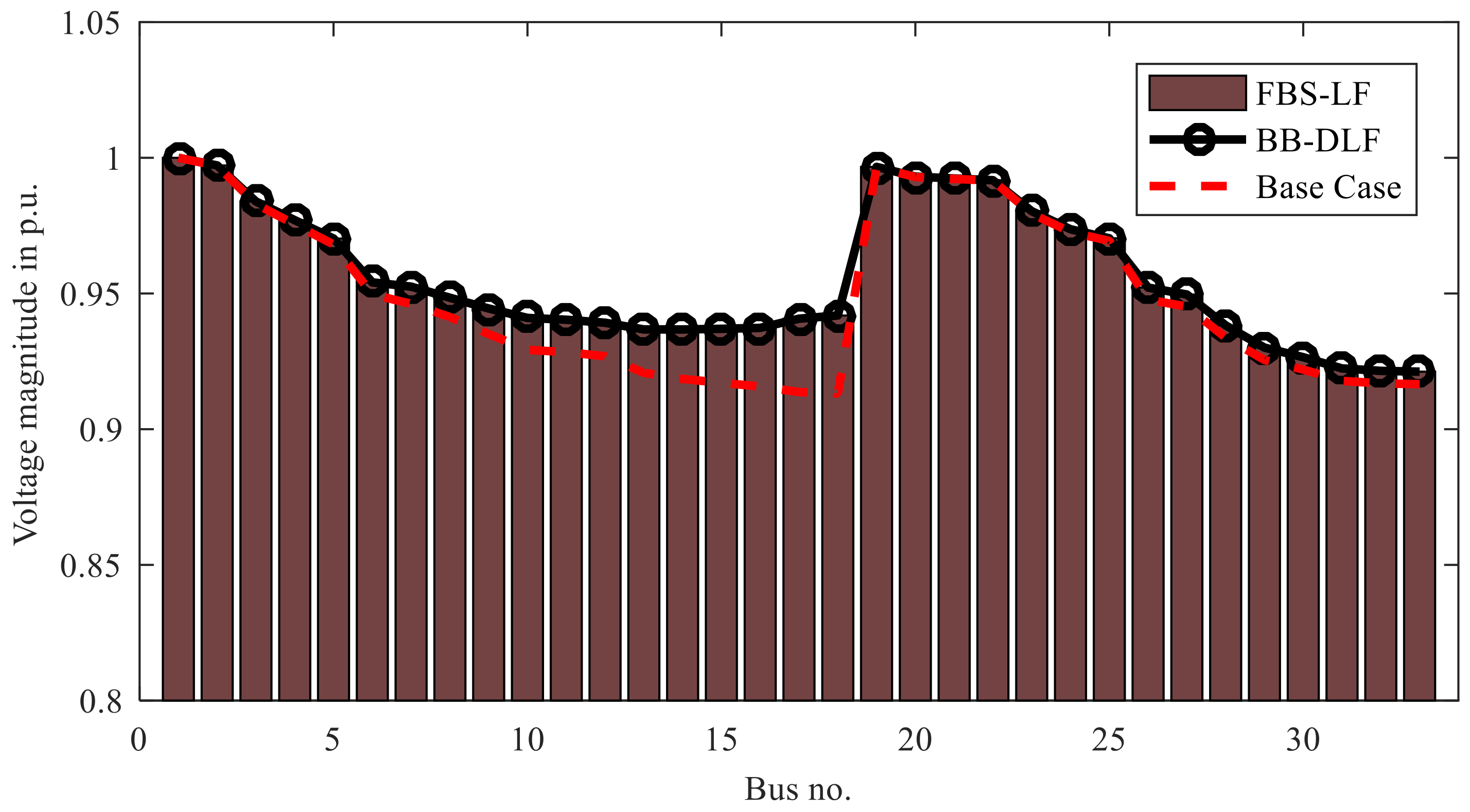
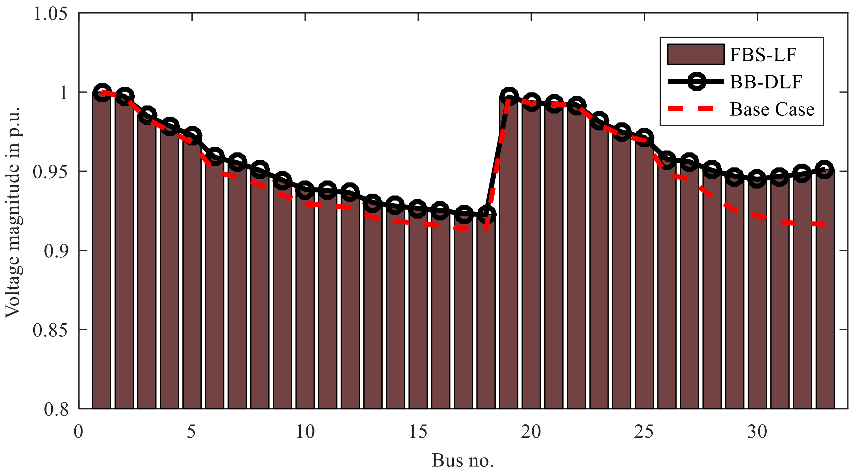
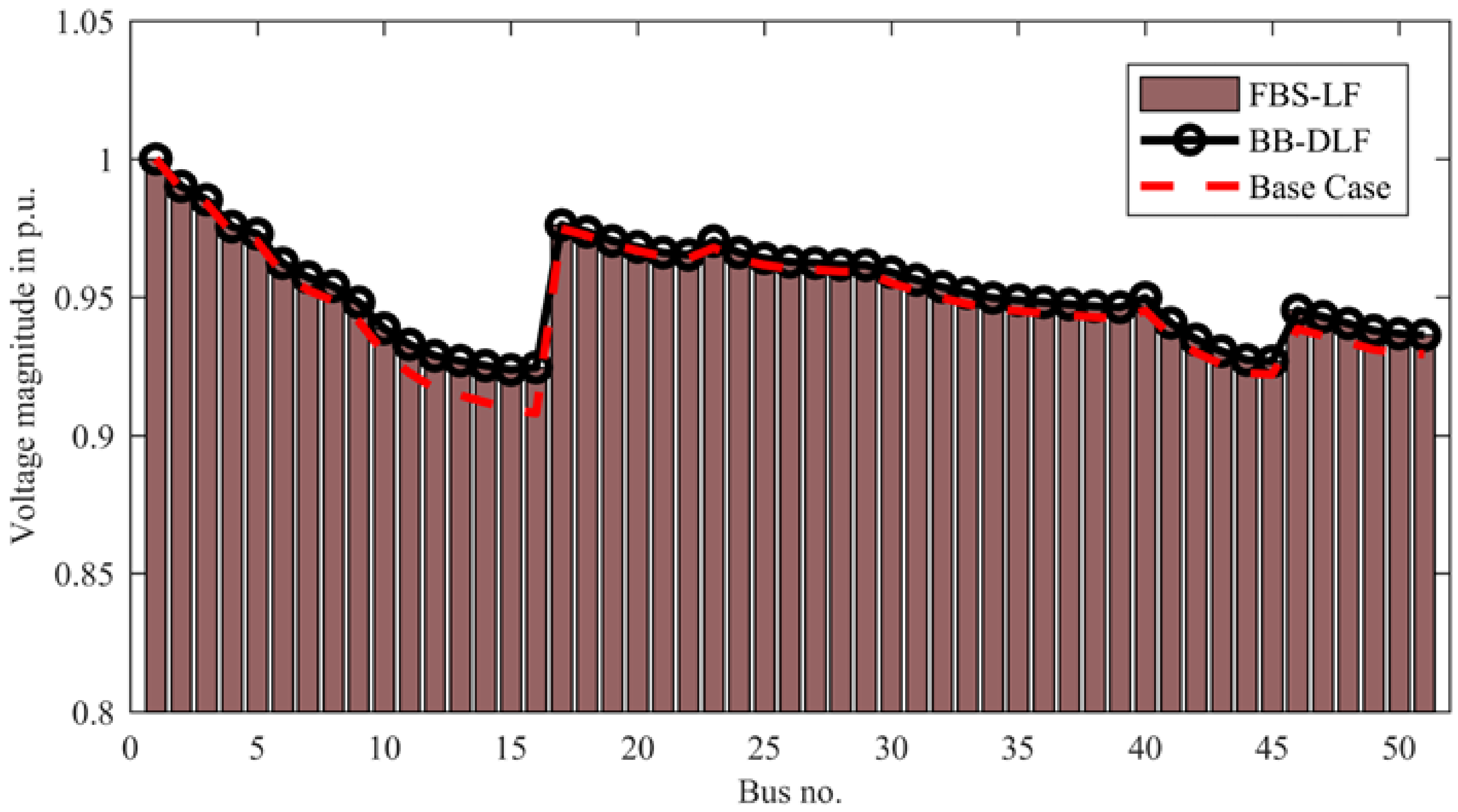
6.1. Integration of D-STATCOM in Load Flow

The robustness and versatility of the suggested PCM–D-STATCOM model are illustrated by combining it with the most widely used distribution load flows: the forward–backward sweep load flow (FBS-LF) and the BB-direct load flow (BB-DLF). For both load flow methodologies, the load flow results of the test systems without and with D-STATCOM allocation are compared. For this purpose, a D-STATCOM of arbitrary size is assigned sequentially to two randomly chosen network buses with poor voltage magnitude for the test systems. Figure 7 and Figure 8 compare the voltage profiles of the 33-bus test system recorded using both load flow methodologies when a D-STATCOM of 500 kVAr and 1000 kVAr is connected to buses 18 and 33, respectively. Similarly, the voltage profile of the 51-bus PDN when a D-STATCOM of 300 kVAr and 1000 kVAr is connected to buses 16 and 9, respectively, is depicted in Figure 9 and Figure 10. It may be noted from Figure 7, Figure 8, Figure 9 and Figure 10 that the voltage magnitude of each bus as obtained by the FBS-LF and BB-DLF are identically the same. Hence, as far as D-STATCOM allocation is concerned, both load flow approaches are equally good.
Table 1 and Table 2 compare the performance of the studied load flow approaches for 33-bus and 51-bus systems for both without and with the sequential allocation of a D-STATCOM. The results indicate that both load flow techniques converged after four iterations; however, the FBS-LF is the quickest. The performance of PDNs is found to be better with a D-STATCOM. However, optimal device assignment may result in the best possible exploitation of the D-STATCOM for overall system performance enhancement. The following sections describe the optimal planning of a PDN with a D-STATCOM.

6.2. Validation of the Proposed D-STATCOM Allocation Method Using SPBO Algorithm

The optimal location and size of D-STATCOM(s) are obtained by minimizing the multiobjective function using the SPBO algorithm for different numbers of the devices. In the present work, the initial class size and maximum iterations of 50 and 100 are set for the SPBO algorithm. The best results out of 30 independent trial runs are considered for OADS. The results for optimal D-STATCOM allocation to minimize real power losses of the 33-bus PDN are compared with the established approaches in Table 3. It can be seen from Table 3 that the proposed SPBO approach is superior compared to the genetic algorithm (GA), immune algorithm (IA), differential evolution (DE) and modified sine cosine algorithm (MoSCA) in minimizing the real power loss of the PDN for a different number of D-STATCOM allocation. Further, the vanishingly small standard deviation (SD) of the objective function proves the robustness of the proposed SPBO approach of solving OADS.
The convergence characteristics of the SPBO algorithm for solving OADS to minimize the MOF in 33-bus and 51-bus PDNs are shown in Figure 11 and Figure 12. It may be noted that the SPBO algorithm converges to the final optimal value within 20 iterations for the 33-bus PDN and within 30 iterations for the 51-bus PDN for one, two and three D-STATCOM allocation.

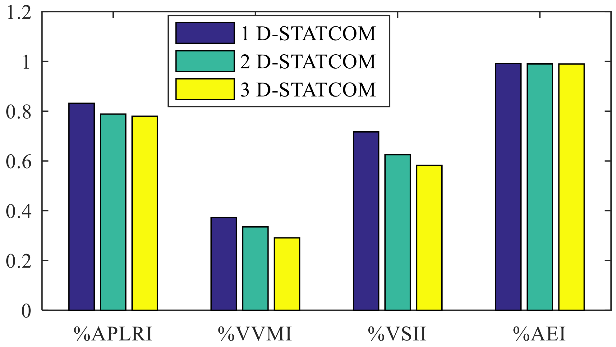
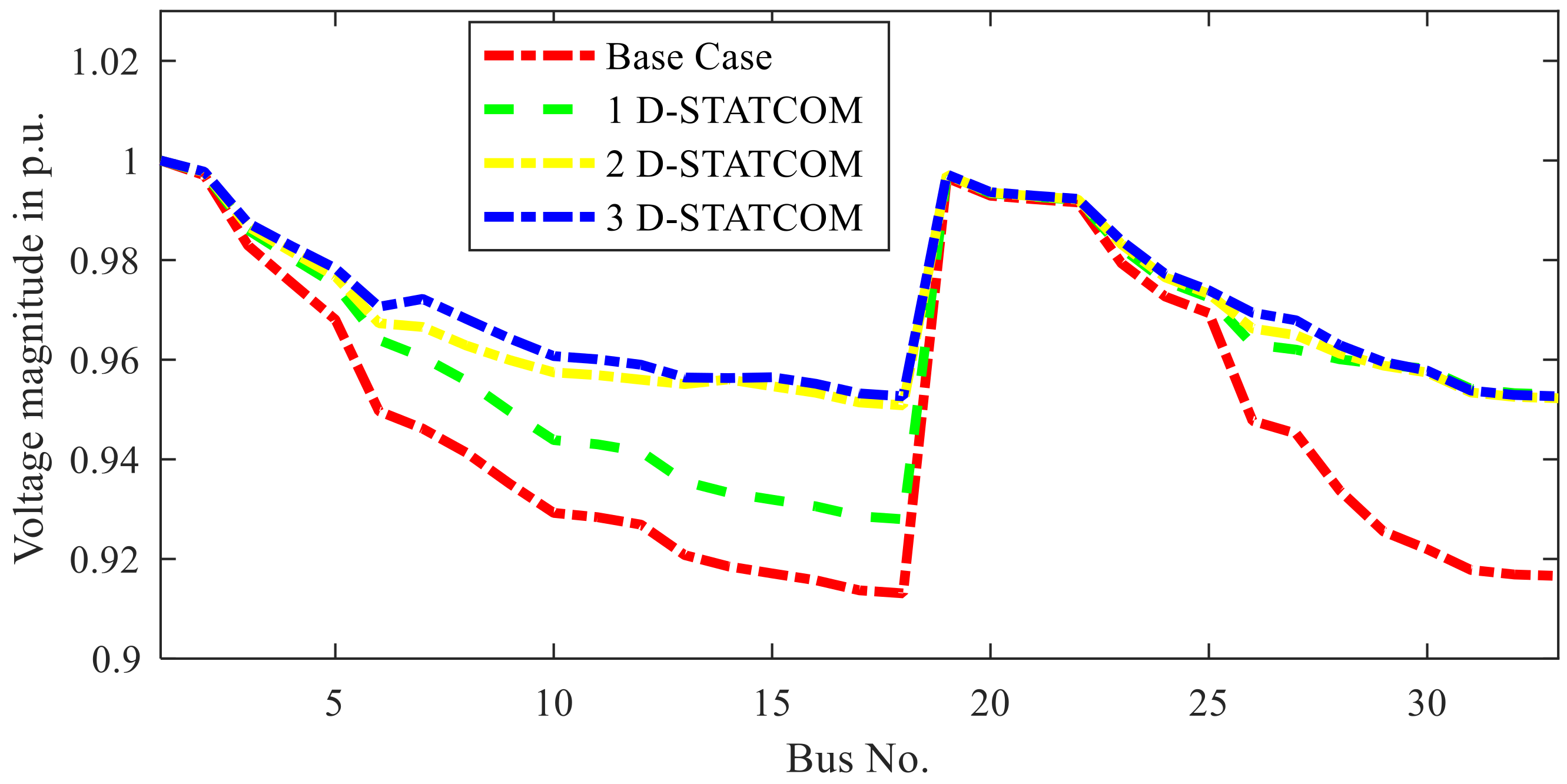
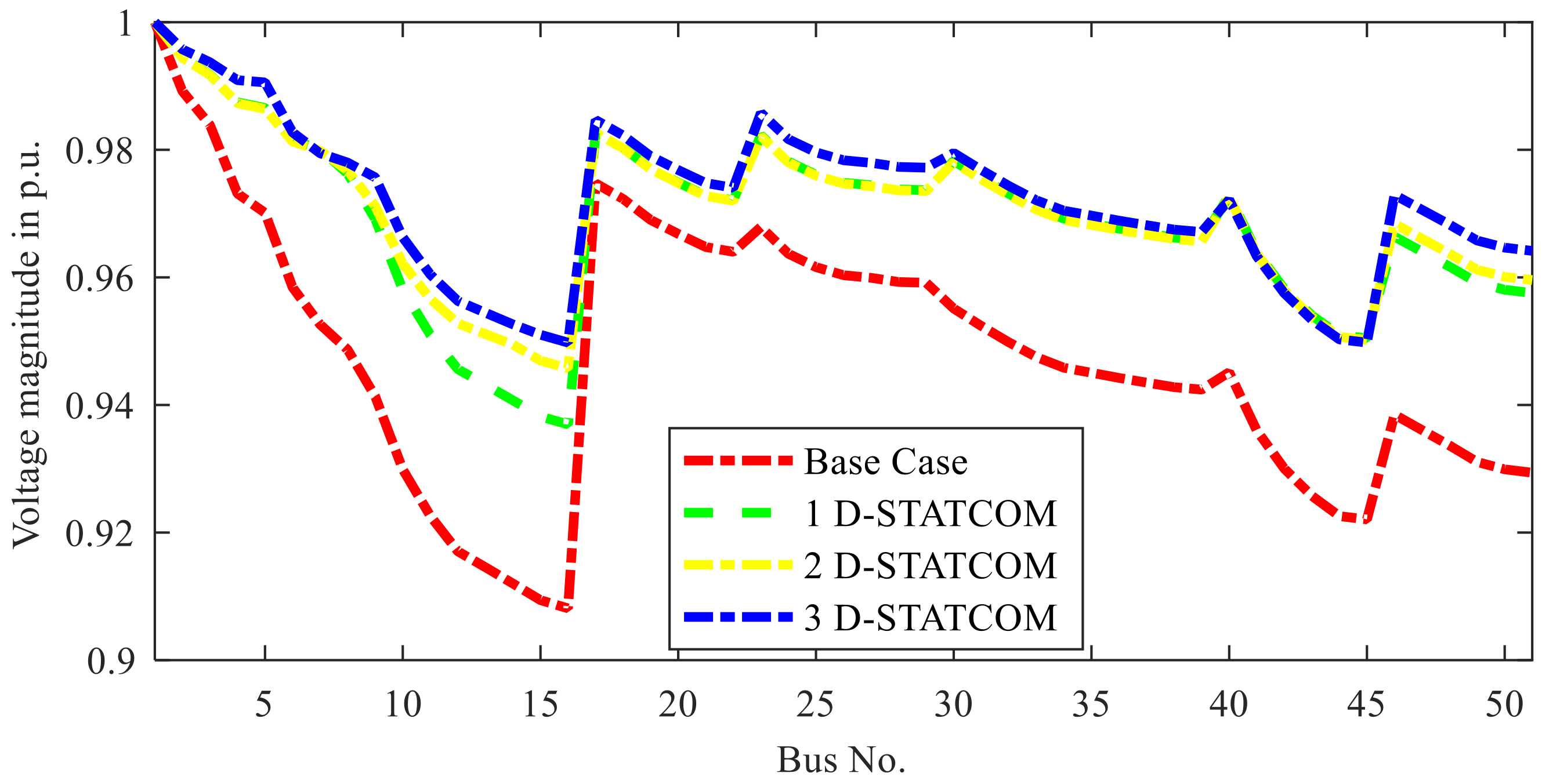
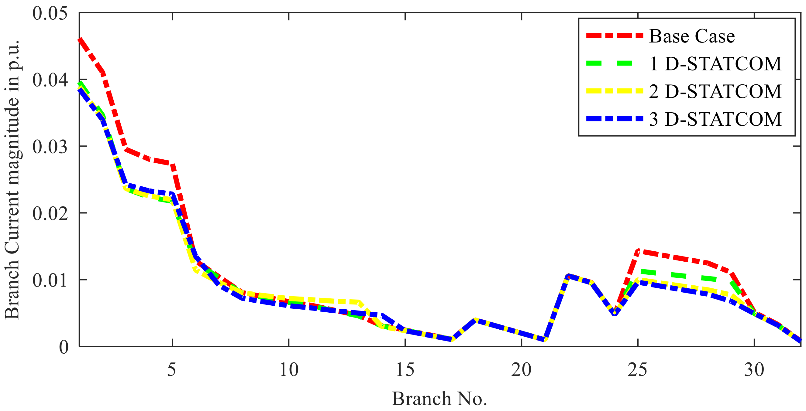
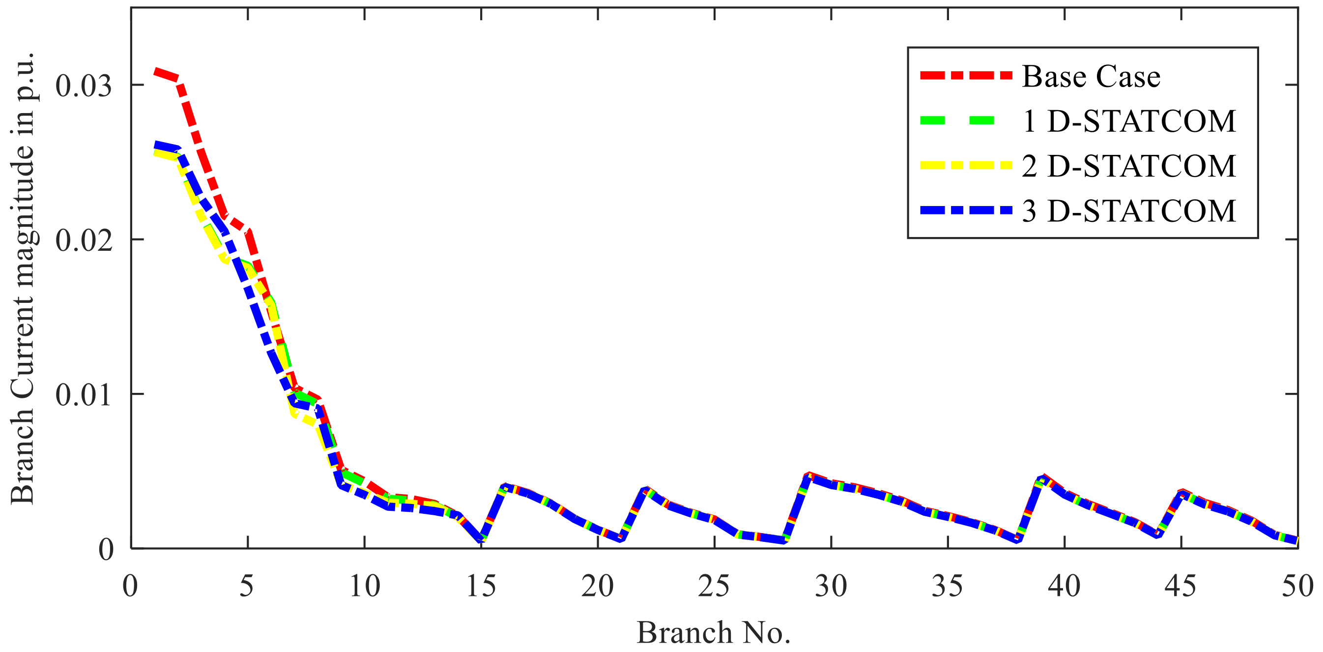
6.3. Performance Analysis of the PDN in Presence of Optimally Allocated D-STATCOMs

Since the D-STATCOM is a costly piece of equipment, the optimal D-STATCOM allocation is obtained to simultaneously optimize both technical and economical indices. The simultaneous optimal placement and rating of one, two and three D-STATCOM units for the minimum multiobjective function are obtained using the SPBO algorithm and are presented in Table 4 and Table 5 for the 33-bus and 51-bus PDNs, respectively. Table 4 and Table 5 also report the real power loss, minimum bus voltage (Vmin), stability index of the critical bus (VSIc), %APLRI, %VVMI, %VSII, %AEI and MOF for the optimal allocation of D-STATCOM(s) for 33-bus and 51-bus PDNs. Table 4 and Table 5 reveal that an optimally allocated D-STATCOM resulted in a much-improved system performance both in terms of technical and economic factors compared to the absence of the D-STATCOM for both of the studied PDNs. Further, the system performance is the best when three D-STATCOM units are optimally allocated than single- and double-unit allocation. In the presence of the three optimally allocated D-STATCOMs, the power loss reduced to 139.1840 kW from 202.6 kW for the 33-bus PDN and 101.0208 kW from 129.5 kW for the 51-bus PDN. Similarly, the minimum bus voltage was improved to 0.9526 p.u. and 0.9498 p.u. with the D-STATCOM from 0.9131 p.u. and 0.9081 p.u. without the D-STATCOM for the 33-bus and 51-bus PDNs, respectively. The voltage stability index of the critical bus also improved from 0.6951 and 0.6801 without the D-STATCOM to 0.8236 and 0.8137 with optimally assigned three D-STATCOMs for the 33-bus and 51-bus PDNs, respectively.
The effect of the optimal D-STATCOM allocation is assessed by the various technical and economic indices of %APLRI, %VVMI, %VSII and %AEI defined in the present work. As seen in Table 4 and Table 5, the values of % APLRI, %VVMI, %VSII and %AEI for optimally assigned three D-STATCOM units are 0.6868, 0.3141, 0.5785 and 0.9843 and 0.7798, 0.2911, 0.5823 and 0.9895, respectively, for the 33-bus and 51-bus PDNs which are significantly lower compared to one and two D-STATCOM allocation. A comparison of the aforementioned indices for one, two and three optimal D-STATCOM allocations for the 33-bus and 51-bus PDNs is also presented in Figure 13 and Figure 14.
Figure 13 and Figure 14 reveal that, for three optimally allocated D-STATCOM units, all four indices are minimum compared to those of optimally allocated one and two D-STATCOM unit(s) for both 33-bus and 51-bus PDNs. Hence, the PDN attains a superior technical performance and economic gain for optimally allocated three D-STATCOM units.
Further, the voltage profile and the branch current variations for the PDN without a D-STATCOM and optimally placed one, two and three D-STATCOMs are compared in Figure 15, Figure 16, Figure 17 and Figure 18 for 33-bus and 51-bus PDNs, respectively.
From Figure 15, it is evident that the voltage profile of the 33-bus PDN is much better in the presence of optimally allocated three D-STATCOMs than in the base case. However, there is a marginal improvement in the voltage profile for three D-STATCOM allocation than two D-STATCOM allocation. Similarly, for the 51-bus PDN, the voltage profile of the PDN in the presence of optimally allocated three D-STATCOMs is far better than that without the allocation of a D-STATCOM as seen in Figure 16. Further, except for a few buses, the voltage profile of the PDN for three D-STATCOM allocation and two D-STATCOM allocation is more or less the same. In terms of the current drawn from the substation, the allocation of one, two and three D-STATCOMs is not significantly different for both PDNs as evident from Figure 17 and Figure 18. However, the current drawn from the substation in the presence of an optimally allocated D-STATCOM is significantly less as compared to without any D-STATCOM for both of the studied PDNs.

6.4. Economic Analysis of the PDN in Presence of Optimally Allocated D-STATCOMs

From the perspective of power distribution network operators (PDNOs), the investment in the augmentation of sophisticated devices for the grid to improve technical performance is justified if it is economically feasible. Hence, a detailed analysis of the annual expenditure of the PDNOs without any device allocation and with the allocation of different numbers of D-STATCOM(s) was carried out in this work. Table 6 reports the annual expenditure and saving thereof for the 33-bus and 51-bus PDNs with no D-STATCOM (base case), one D-STATCOM, two D-STATCOMs and three D-STATCOMs. The result reveals that without any device allocation, the 33-bus and 51-bus PDNOs incur an annual expenditure of USD 2.6895 × 10⁶ and USD 1.7802 × 10⁶, respectively. Meanwhile, with one, two and three optimally assigned D-STATCOM(s), the PDNOs have savings of USD 3.8016 × 10⁴, USD 4.0643 × 10⁴ and USD 4.2323 × 10⁴ for the 33-bus PDN and USD 1.4221 × 10⁴, USD 1.8049 × 10⁴ and USD 1.8684 × 10⁴ for the 51-bus PDN.

7. Conclusions

This work presents a detailed revisit of the modeling features of D-STATCOMs. A new D-STATCOM modeling approach based on current injection was proposed. The proposed D-STATCOM model was coupled with two notable distribution system load flow programs, namely the forward–backward sweep load flow and the BIBC- and BCBV-matrix-based direct load flow, and the results demonstrate the versatility of the proposed D-STATCOM modeling. Furthermore, the optimal allocation of the D-STATCOM was carried out with the goal of improving the technical performance of the PDN and minimizing the PDN’s annual investment cost. To solve the optimal allocation of the D-STATCOM in a multiobjective framework comprising several technical and economic indicators, the APLRI, VVMI, VSII and AEI, a new parameter-free metaheuristic method, namely a student-psychology-based optimization algorithm, was presented. When compared to other metaheuristic techniques such as DE, GA, IA and MoSCA, the results show that the SPBO algorithm is more efficient and robust in solving OADS. When three D-STATCOMs are optimally deployed, the real power loss is decreased to 139 kW from 202 kW for a 33-bus PDN and to 101 kW from 129 kW for a practical 51-bus PDN. Similarly, for optimally assigned three D-STATCOM units, the reduction in voltage deviation and improvement in the voltage stability index for the 33-bus PDN and 51-bus PDN were 0.9526 p.u., 0.8326 and 0.9498 p.u., 0.8137, respectively. Further, the joint optimization of the technical and economic indices resulted in savings of USD 3.8016 × 10⁴, USD 4.0643 × 10⁴ and USD 4.2323 × 10⁴ for the 33-bus PDN and USD 1.4221 × 10⁴, USD 1.8049 × 10⁴ and USD 1.8684 × 10⁴ for the 51-bus PDN with one, two and three optimally assigned D-STATCOM(s).

Author Contributions

Conceptualization, S.K.D., S.M. and A.Y.A.; methodology, S.K.D. and S.M.; software, S.K.D., S.M. and A.Y.A.; validation, S.K.D., S.M. and A.Y.A.; formal analysis, S.K.D. and A.Y.A.; investigation, S.K.D., S.M. and A.Y.A.; resources, S.K.D. and S.M.; data curation, S.K.D. and S.M.; writing—original draft preparation, S.K.D., S.M. and A.Y.A.; writing—review and editing, S.K.D., S.M. and A.Y.A.; visualization, S.K.D. and S.M.; supervision, S.K.D., S.M. and A.Y.A.; project administration, S.M. and A.Y.A.; funding acquisition, S.M. and A.Y.A. All authors have read and agreed to the published version of the manuscript.

Funding

This research received no external funding.

Institutional Review Board Statement

Not applicable.

Informed Consent Statement

Not applicable.

Conflicts of Interest

The authors declare no conflict of interest.

References

  1. Bollen, M.H. What is power quality? Electr. Power Syst. Res. 2003, 66, 5–14. [Google Scholar] [CrossRef]
  2. Pan, J.; Teklu, Y.; Rahman, S.; Jun, K. Review of usage-based transmission cost allocation methods under open access. IEEE Trans. Power Syst. 2000, 15, 1218–1224. [Google Scholar]
  3. Hosseini, M.; Shayanfar, H.A.; Fotuhi-Firuzabad, M. Modeling of unified power quality conditioner (UPQC) in distribution systems load flow. Energy Convers. Manag. 2009, 50, 1578–1585. [Google Scholar] [CrossRef]
  4. Gupta, A.R.; Kumar, A. Impact of various load models on D-STATCOM allocation in DNO operated distribution network. Procedia Comput. Sci. 2018, 125, 862–870. [Google Scholar] [CrossRef]
  5. Hingorani, N.G. Introducing custom power. IEEE Spectr. 1995, 32, 41–48. [Google Scholar] [CrossRef]
  6. Committee of the IEEE Power and Energy Society. IEEE Guide for Application of Power Electronics for Power Quality Improvement on Distribution Systems Rated 1 kV Through 38 kV. Sponsored by the Transmission and Distribution Committee IEEE Power & Energy Society 2012. Available online: https://ieeexplore.ieee.org/document/6190701/citations#citations (accessed on 18 September 2022).
  7. Sanam, J.; Panda, A.K.; Ganguly, S. Optimal phase angle injection for reactive power compensation of distribution systems with the allocation of multiple distribution STATCOM. Arab. J. Sci. Eng. 2017, 42, 2663–2671. [Google Scholar] [CrossRef]
  8. Hosseini, M.; Shayanfar, H.A.; Fotuhi-Firuzabad, M. Modeling of D-STATCOM in distribution systems load flow. J. Zhejiang Univ.-Sci. A 2007, 8, 1532–1542. [Google Scholar] [CrossRef]
  9. Banerji, A.; Biswas, S.K.; Singh, B. D-STATCOM control algorithms: A review. Int. J. Power Electron. Drive Syst. 2012, 2, 285. [Google Scholar]
  10. Ramsay, S.M.; Cronin, P.E.; Nelson, R.J.; Bian, J.; Menendez, F.E. Using distribution static compensators (D-STATCOMs) to extend the capability of voltage-limited distribution feeders. In Proceedings of the Rural Electric Power Conference, Fort Worth, TX, USA, 28–30 April 1996; p. A4-18. [Google Scholar]
  11. Jazebi, S.; Hosseinian, S.H.; Vahidi, B. D-STATCOM allocation in distribution networks considering reconfiguration using differential evolution algorithm. Energy Convers. Manag. 2011, 52, 2777–2783. [Google Scholar] [CrossRef]
  12. Dehnavi, H.D.; Esmaeili, S. A new multiobjective fuzzy shuffled frog-leaping algorithm for optimal reconfiguration of radial distribution systems in the presence of reactive power compensators. Turk. J. Electr. Eng. Comput. Sci. 2013, 21, 864–881. [Google Scholar] [CrossRef]
  13. Sedighizadeh, M.; Eisapour-Moarref, A. The imperialist competitive algorithm for optimal multi-objective location and sizing of D-STATCOM in distribution systems considering loads uncertainty. INAE Lett. 2017, 2, 83–95. [Google Scholar] [CrossRef]
  14. Hussain, S.S.; Subbaramiah, M. An analytical approach for optimal location of D-STATCOM in radial distribution system. In Proceedings of the 2013 International Conference on Energy Efficient Technologies for Sustainability, Nagercoil, India, 10–12 April 2013; pp. 1365–1369. [Google Scholar]
  15. Devi, S.; Geethanjali, M. Optimal location and sizing determination of Distributed Generation and D-STATCOM using Particle Swarm Optimization algorithm. Int. J. Electr. Power Energy Syst. 2014, 62, 562–570. [Google Scholar] [CrossRef]
  16. Sanam, J.; Ganguly, S.; Panda, A.K. Distribution STATCOM with optimal phase angle injection model for reactive power compensation of radial distribution networks. Int. J. Numer. Model. Electron. Netw. Devices Fields 2017, 30, e2240. [Google Scholar] [CrossRef]
  17. Samal, P.; Mohanty, S.; Ganguly, S. Modelling and allocation of a D-STATCOM on the performance improvement of unbalanced radial distribution systems. J. Electr. Eng. 2016, 16, 323–332. [Google Scholar]
  18. Gupta, A.R.; Kumar, A. Optimal placement of D-STATCOM using sensitivity approaches in mesh distribution system with time variant load models under load growth. Ain Shams Eng. J. 2018, 9, 783–799. [Google Scholar] [CrossRef]
  19. Gupta, A.R.; Kumar, A. Energy saving using D-STATCOM placement in radial distribution system under reconfigured network. Energy Procedia 2016, 90, 124–136. [Google Scholar] [CrossRef]
  20. Yuvaraj, T.; Ravi, K.; Devabalaji, K.R. DSTATCOM allocation in distribution networks considering load variations using bat algorithm. Ain Shams Eng. J. 2017, 8, 391–403. [Google Scholar] [CrossRef]
  21. Yuvaraj, T.; Ravi, K. Multi-objective simultaneous DG and DSTATCOM allocation in radial distribution networks using cuckoo searching algorithm. Alex. Eng. J. 2018, 57, 2729–2742. [Google Scholar] [CrossRef]
  22. Kanwar, N.; Gupta, N.; Niazi, K.R.; Swarnkar, A. Improved cat swarm optimization for simultaneous allocation of DSTATCOM and DGs in distribution systems. J. Renew. Energy 2015, 2015, 189080. [Google Scholar] [CrossRef]
  23. Arya, A.K.; Kumar, A.; Chanana, S. Analysis of distribution system with D-STATCOM by gravitational search algorithm (GSA). J. Inst. Eng. (India) Ser. B 2019, 100, 207–215. [Google Scholar] [CrossRef]
  24. Dash, S.K.; Mishra, S. Simultaneous Optimal Placement and Sizing of D-STATCOMs Using a Modified Sine Cosine Algorithm. In Advances in Intelligent Computing and Communication; Springer: Singapore, 2021; pp. 423–436. [Google Scholar]
  25. Dash, S.K.; Mishra, S.; Raut, U.; Abdelaziz, A.Y. Optimal Allocation of DSTATCOM Units in Electric Distribution Network Using Improved Symbiotic Organisms Search Algorithms. In Proceedings of the 2021 International Conference in Advances in Power, Signal, and Information Technology (APSIT), Bhubaneswar, India, 8–10 October 2021; pp. 1–6. [Google Scholar]
  26. Sanam, J. Optimization of planning cost of radial distribution networks at different loads with the optimal placement of distribution STATCOM using differential evolution algorithm. Soft Comput. 2020, 24, 13269–13284. [Google Scholar] [CrossRef]
  27. Dash, S.K.; Mishra, S.; Raut, U.; Abdelaziz, A.; Hong, J.; Geem, Z.W. Optimal Planning of Multitype DGs and D-STATCOMs in Power Distribution Network using an Efficient Parameter Free Metaheuristic Algorithm. Energies 2022, 15, 3433. [Google Scholar] [CrossRef]
  28. Das, B.; Mukherjee, V.; Das, D. Student psychology-based optimization algorithm: A new population-based optimization algorithm for solving optimization problems. Adv. Eng. Softw. 2020, 146, 102804. [Google Scholar] [CrossRef]
  29. Balu, K.; Mukherjee, V. Optimal siting and sizing of distributed generation in radial distribution system using a novel student psychology-based optimization algorithm. Neural Comput. Appl. 2021, 33, 15639–15667. [Google Scholar] [CrossRef]
  30. Roy, R.; Mukherjee, V.; Singh, R.P. Model order reduction of proton exchange membrane fuel cell system using student psychology based optimization algorithm. Int. J. Hydrog. Energy 2021, 46, 37367–37378. [Google Scholar] [CrossRef]
  31. Das, B.; Barik, S.; Mukherjee, V.; Das, D. Application of mixed discrete student psychology-based optimization for optimal placement of unity power factor distributed generation and shunt capacitor. Int. J. Ambient. Energy 2022, accepted. [Google Scholar] [CrossRef]
  32. Mishra, S.; Das, D.; Paul, S. A simple algorithm for distribution system load flow with distributed generation. In Proceedings of the IEEE International Conference on Recent Advances and Innovations in Engineering (ICRAIE), Jaipur, India, 9–11 May 2014. [Google Scholar]
  33. Teng, J.H. A direct approach for distribution system load flow solutions. IEEE Trans. Power Deliv. 2003, 18, 882–887. [Google Scholar] [CrossRef]
  34. Chakravorty, M.; Das, D. Voltage stability analysis of radial distribution networks. Int. J. Electr. Power Energy Syst. 2001, 23, 129–135. [Google Scholar] [CrossRef]
  35. Mishra, S.; Das, D.; Paul, S. A comprehensive review on power distribution network reconfiguration. Energy Systems 2017, 8, 227–284. [Google Scholar] [CrossRef]
  36. Gampa, S.R.; Das, D. Optimum placement and sizing of DGs considering average hourly variations of load. Int. J. Electr. Power Energy Syst. 2015, 66, 25–40. [Google Scholar] [CrossRef]
  37. Taher, S.A.; Afsari, S.A. Optimal location and sizing of DSTATCOM in distribution systems by immune algorithm. Int. J. Electr. Power Energy Syst. 2014, 60, 34–44. [Google Scholar] [CrossRef]
Figure 1. Schematic representation of D-STATCOM modeled as (a) PQ Bus and (b) PV Bus.
Energies 15 06908 g001
Figure 2. Single-line diagram of two consecutive nodes of a PDN.
Energies 15 06908 g002
Figure 3. Phasor diagram of two consecutive nodes of a PDN.
Energies 15 06908 g003
Figure 4. Single-line diagram of two consecutive nodes of a PDN with D-STATCOM at (t + 1)th node.
Energies 15 06908 g004
Figure 5. Phasor diagram of two consecutive nodes of a PDN with D-STATCOM at (t + 1)th node.
Energies 15 06908 g005
Figure 6. Flow Chart for implementing SPBO for OADS.
Energies 15 06908 g006
Figure 7. Comparison of voltage profile of PDN as obtained by FBS-LF and BB-DLF when a 500 kVAr D-STATCOM is allocated to bus 18 of 33-bus PDN.
Energies 15 06908 g007
Figure 8. Comparison of voltage profile of PDN as obtained by FBS-LF and BB-DLF when a 1000 kVAr D-STATCOM is allocated to bus 33 of 33-bus PDN.
Energies 15 06908 g008
Figure 9. Comparison of voltage profile of PDN as obtained by FBS-LF and BB-DLF when a 300 kVAr D-STATCOM is allocated to bus 16 of 51-bus PDN.
Energies 15 06908 g009
Figure 10. Comparison of voltage profile of PDN as obtained by FBS-LF and BB-DLF when a 1000 kVAr D-STATCOM is allocated to bus 9 of 51-bus PDN.
Energies 15 06908 g010
Figure 11. Convergence characteristics for OADS in 33-bus PDN.
Energies 15 06908 g011
Figure 12. Convergence characteristics for OADS in 51-bus PDN.
Energies 15 06908 g012
Figure 13. Comparison of performance indices for OADS in 33-bus PDN.
Energies 15 06908 g013
Figure 14. Comparison of performance indices for OADS in 51-bus PDN.
Energies 15 06908 g014
Figure 15. Comparison of voltage profile with and without D-STATCOMs of 33-bus PDN.
Energies 15 06908 g015
Figure 16. Comparison of voltage profile with and without D-STATCOMs of 51-bus PDN.
Energies 15 06908 g016
Figure 17. Comparison of current profile with and without D-STATCOMs of 33-bus PDN.
Energies 15 06908 g017
Figure 18. Comparison of current profile with and without D-STATCOMs of 51-bus PDN.
Energies 15 06908 g018
Table 1. Comparison of Performance of Load Flow for incorporation of proposed D-STATCOM Modeling into 33-Bus PDN.
ParametersBase Case500 kVAr @ 181000 kVAr @ 33
FBS-LFDLFFBS-LFDLFFBS-LFDLF
Simulation Time, Sec0.0030750.0051300.0046850051650.0033210.005137
No. of Iteration444444
Ploss, kW202.6650202.6650182.5309182.4719154.4535154.3767
Qloss, kVAr135.1327135.1327123.3050123.2629106.5591106.5066
Vmin, p.u.0.91310.91310.92120.92120.92260.9226
SImin, p.u.0.69510.69510.72010.72010.72460.7246
Table 2. Comparison of Performance of Load Flow for incorporation of proposed D-STATCOM Modeling into 51-Bus PDN.
ParametersBase Case300 kVAr @ 161000 kVAr @ 9
FBS-LFBB-DLFFBS-LFBB-DLFFBS-LFBB-DLF
Simulation Time, Sec0.0060320.0104960.0089240.0104700.0062140.013345
No. of Iteration444444
Ploss, kW129.5500129.5500115.9553115.9209104.5432103.9642
Qloss, kVAr111.6786111.678698.521798.497084.897984.3043
Vmin, p.u.0.90810.90810.92370.92380.93190.9321
SImin, p.u.0.68010.68010.72410.72420.75420.7549
Table 3. Comparison of OADS using different methods for 33-bus PDN.
MethodsNdstatLocationD-STATCOM Size, MVArPloss, kWWorst
Ploss,
kW
Average
Ploss,
kW
SD of Ploss, kW
Base case0202.6---
MoSCA [24]1301.3060143.5---
Proposed1301.3154143.5143.5963143.59631.04 × 10−14
GA [37]1121114.2173.9---
IA [37]1120.9624171.8---
DE [26]1301.2527143.5---
MoSCA [24]230
10
0.6645
1.0561
137.8---
Proposed230
12
1.1109
0.4936
135.7135.7480135.74801.04 × 10−9
MoSCA [24]330
4
11
0.7713
0.9933
0.4251
135.2---
Proposed324
13
30
0.5555
0.4005
1.0890
132.1132.1685132.16833.48 × 10−5
Table 4. Comparison of results for OADS using SPBO algorithm for 33-bus PDN.
Optimal BusOptimal D-STATCOM Rating, MVArRPL, kWVmin,
p.u.
VSIc%APLRI%VVMI%VSII%AEIMOF
301.5810145.99160.92800.74150.72040.53690.84770.98590.7139
14
30
0.7012
1.2669
141.83670.95080.81740.69990.34660.59900.98490.6360
15
7
30
0.4651
0.8283
1.0419
139.18400.95260.82360.68680.31410.57850.98430.6190
Table 5. Comparison of results for OADS using SPBO algorithm for 51-bus PDN.
Optimal BusOptimal D-STATCOM Rating, MVArRPL, kWVmin,
p.u.
VSIc%APLRI%VVMI%VSII%AEIMOF
71.7763107.76850.93690.77070.83190.37260.71690.99200.7360
7
14
1.4473
0.3142
102.13990.94570.79990.78840.33510.62540.98990.6917
5
15
9
1.2129
0.2428
0.7508
101.02080.94980.81370.77980.29110.58230.98950.6727
Table 6. Economic analysis of the PDNs with and without allocation of D-STATCOMs.
ParametersPDNBase CaseNdstat = 1Ndstat = 2Ndstat = 3
AE0 (USD)(33-bus)2.6895 × 10⁶---
(51-bus)1.7802 × 10⁶---
AEdstat (USD)(33-bus)-2.6515 × 1062.6489 × 1062.6472 × 106
(51-bus)-1.7660 × 1061.7621 × 1061.7615 × 106
Savings =
AE0–AEdstat (USD)
(33-bus)-3.8016 × 1044.0643 × 1044.2323 × 104
(51-bus)-1.4221 × 1041.8049 × 1041.8684 × 104
Publisher’s Note: MDPI stays neutral with regard to jurisdictional claims in published maps and institutional affiliations.

