Abstract
Prognostics and Health Management (commonly called PHM) is a field that focuses on the degradation mechanisms of systems in order to estimate their health status, anticipate their failure and optimize their maintenance. PHM uses methods, tools and algorithms for monitoring, anomaly detection, cause diagnosis, prognosis of the remaining useful life (RUL) and maintenance optimization. It allows for permanently monitoring the health of the system and provides operators and managers with relevant information to decide on actions to be taken to maintain the system in optimal operational conditions. This paper aims to present the emergence of the PHM thematically to describe the subjacent processes, particularly prognosis, how it supplies the different maintenance strategies and to explain the benefits that can be anticipated. More specifically, this paper establishes a state of the art in prognostic methods used today in the PHM strategy. In addition, this paper shows the multitude of possible prognostic approaches and the choice of one among them that will help to provide a framework for industrial companies.
1. Introduction
With the challenge of the industries to maintain their equipment at maximum reliability, availability, profitability and safety with minimum maintenance cost, maintenance strategies such the PHM (Prognostics and Health Management) have been developed. This strategy is applied to industrial systems requiring higher reliability standards. This imposes a major challenge for many industries such as aerospace, aeronautics, automotive, manufacturing sectors, electronic systems, energy systems, rotating machinery and health sciences [1,2,3,4]. In order to satisfy the requirements cited above, many works have been carried out on the subject of PHM. Great efforts have been made over the past twenty years by researchers and industrialists to find methods for preventing and predicting failures [5,6,7,8,9,10]. These methods have been developed in different fields of application and can be grouped under the term PHM. Upstream goals behind implementing a PHM architecture include:
- -
- Better availability and a consequent reduction in operating and maintenance costs, due to a strategy based on monitoring the state of the system;
- -
- Improved reliability and safety of operational units;
- -
- Faster detection of performance degradation or loss for increased operating efficiency.
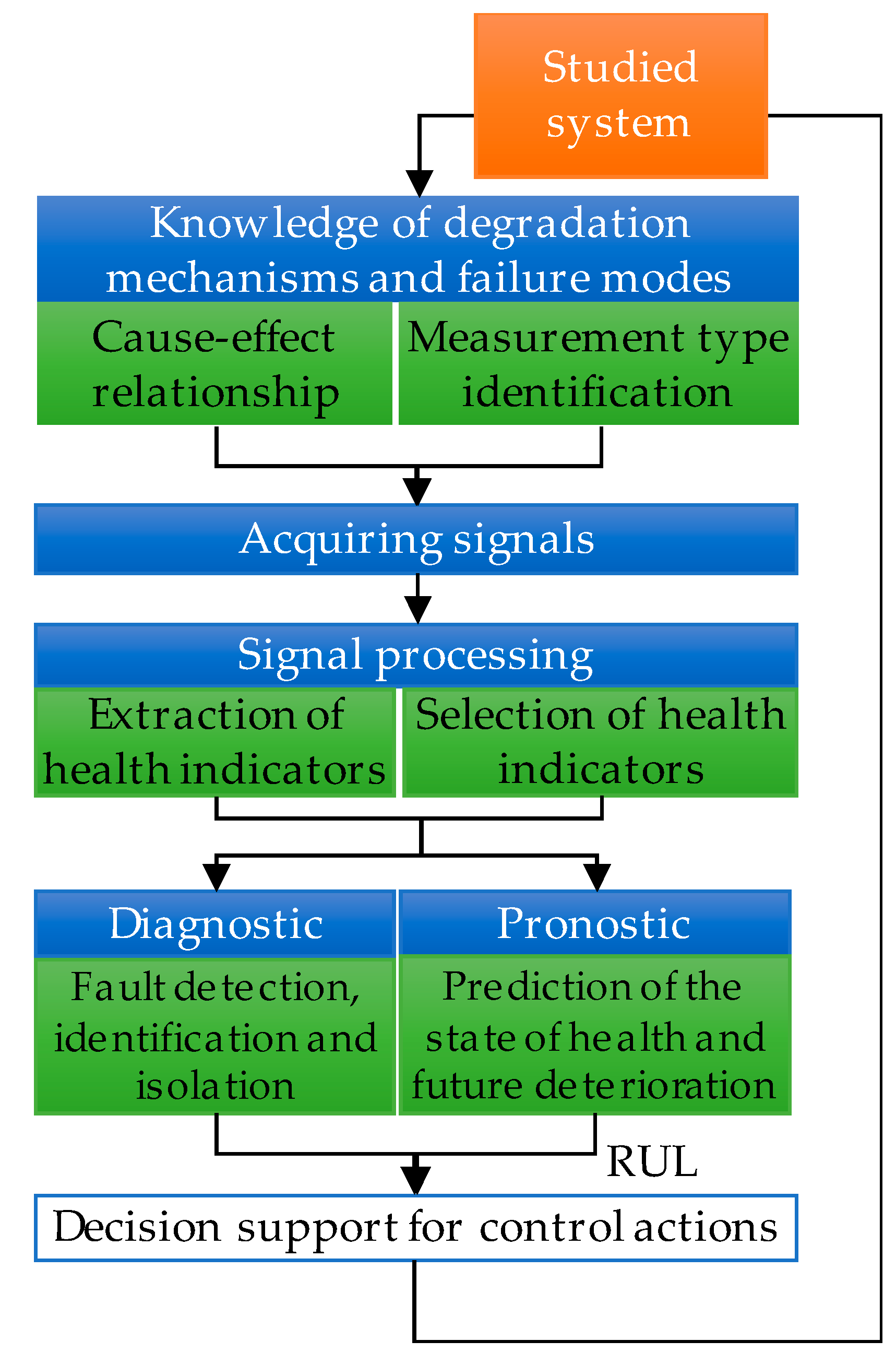
The downstream objective of implementing a PHM architecture includes monitoring the condition of the system for predictive maintenance. As shown in Figure 1, PHM is defined as a strategy to detect, diagnose and predict the future state of a system. This process is carried out using the modules described below: knowledge of degradation mechanisms and failure modes, data acquisition, data pre-processing, diagnosis and prognosis, and decision support.
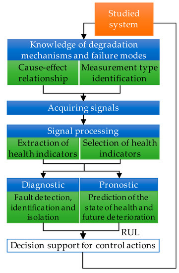
Figure 1.
Architecture of the PHM process.
As can be seen from Figure 1, the prognosis is an essential step for the implementation of a PHM strategy. Its purpose is to estimate the remaining useful life (RUL) of the selected components, i.e., the remaining operating time before these components fail or no longer operate sufficiently satisfactorily. This makes it possible to adapt and optimize the maintenance schedule. This step defines the difference between a predictive maintenance policy and the condition-based maintenance.
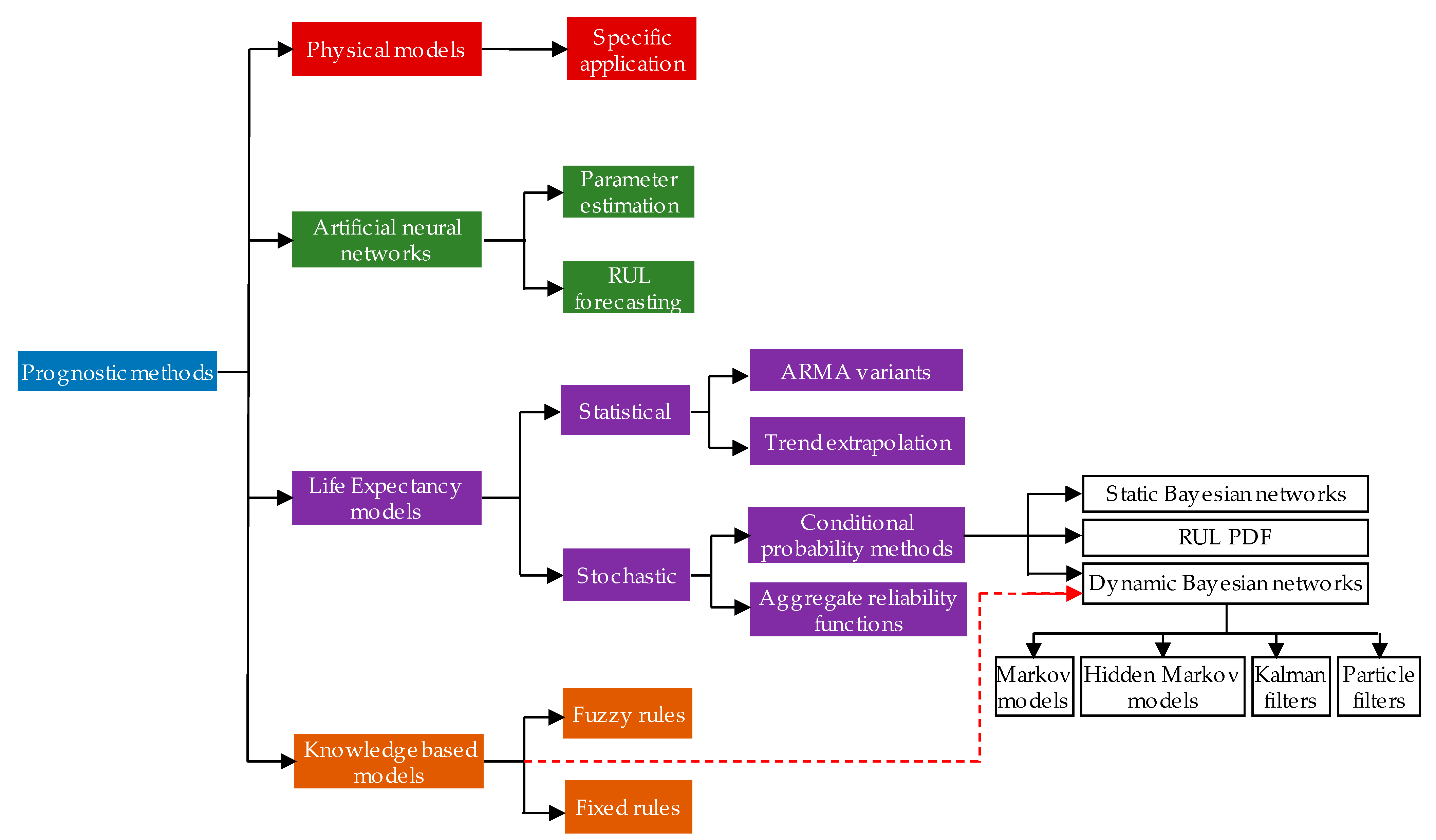
The prognosis has been the subject of growing interest for several decades, and several methods have been developed, tested and improved. Categorizing these methods into distinct classes proves to be complicated by the diversity of tasks to be performed. For instance, Roemer et al. in [11] categorize prognostic methods into three types as shown in Figure 2:

Figure 2.
Prognostic approaches [11].
- -
- Prognosis based on physical models, which relies on mathematical and/or physical models of degradation phenomena;
- -
- Data-based prognosis, which consists of analyzes of datasets for the search for health indicators of the state of health of the component;
- -
- Prognosis based on experience, which is based on the exploitation of knowledge acquired by the failure or degradation of the component in the past.
Nevertheless, it is conceivable to include experience-based prognosis in data-driven prognosis since it processes the system data. Thus, the classification into model-based, data-based and artificial intelligence given in [12,13] will be considered. Hence, a classification of prognostic categories delivered by [11] is shown in Figure 3.
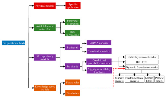
Figure 3.
Prognostic methods classification [11].
This classification evolved over time as shown in Table 1. The study and analysis of the different classifications proposed in the literature, and summarized in Table 1, led us to note that the groupings of methods proposed were organized by the type of data and the formalization tools used. In addition, we note that the model-based approach often comes up, and the other approaches have similarities with each other in the tools they use. Based on this observation, the PHM community tends more and more toward a unified and consensual classification between the different proposals published in the literature.

Table 1.
Evolution of the classification of prognostic methods.
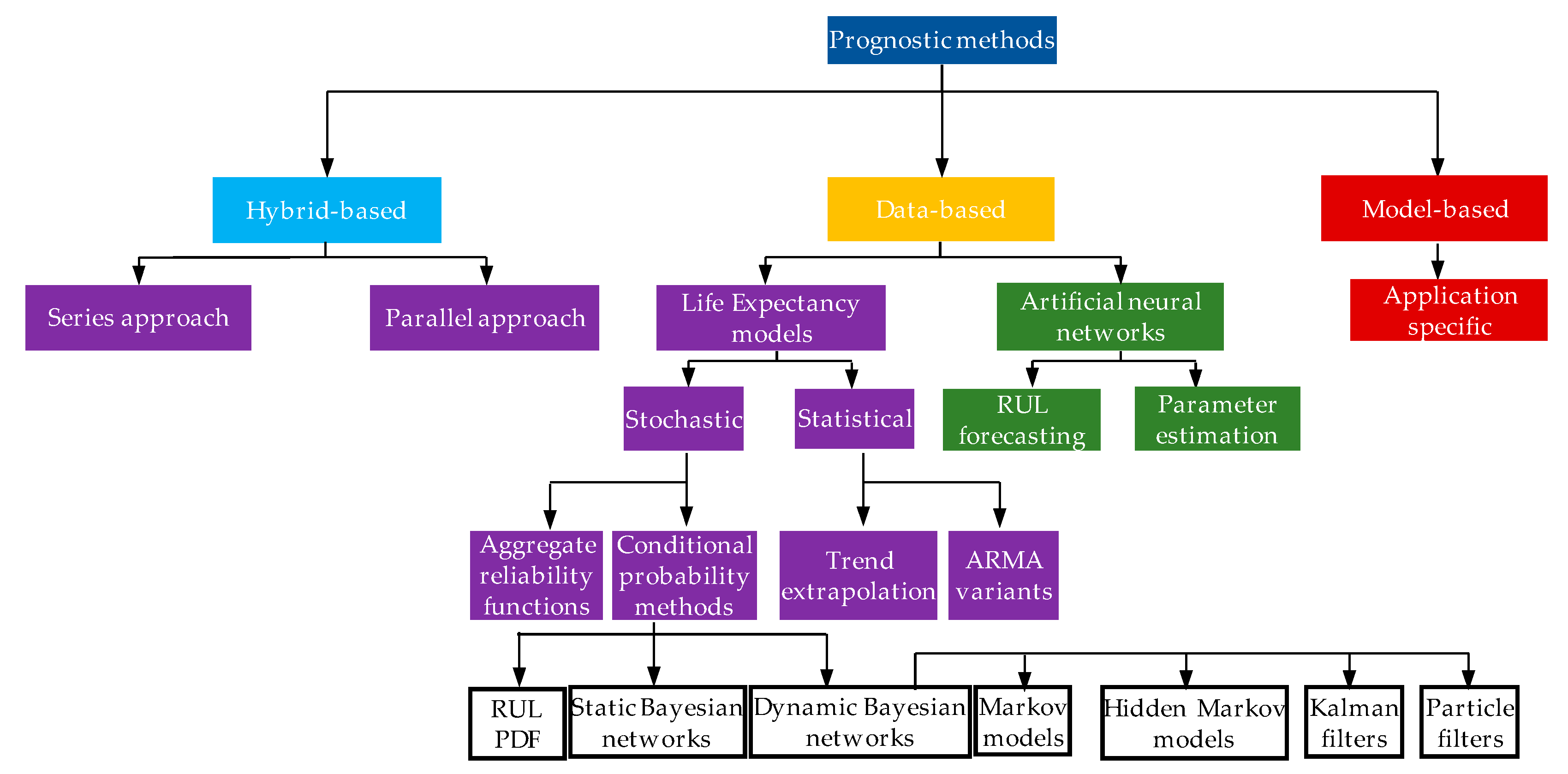
On the basis of this study, we propose to follow the following classification illustrated in Figure 4:

Figure 4.
Classification of prognostics approaches.
- −
- the prognosis based on a physical model;
- −
- data-driven prognosis;
- −
- the hybrid prognosis.
To these three categories, we added several criteria in order to identify the applicability of each category as shown in Table 2.

Table 2.
Applicability of the prognosis approaches.
Hence, this work details the prognostic layer of the PHM architecture and provides prognostic methods treated in the literature and which are used in the Prognostics and Health Management strategy. Thus, it lists the various possible approaches and establishes the choice of a method among prognostic techniques which will represent a major interest in the industry. Therefore, sections of this work are centered around the detailed presentation of prognostic methods used in the domain of the PHM strategy and their categorization. In the next section, this aspect is detailed.
2. Prognostic Methods Categorization
2.1. Model-Based Prognostic
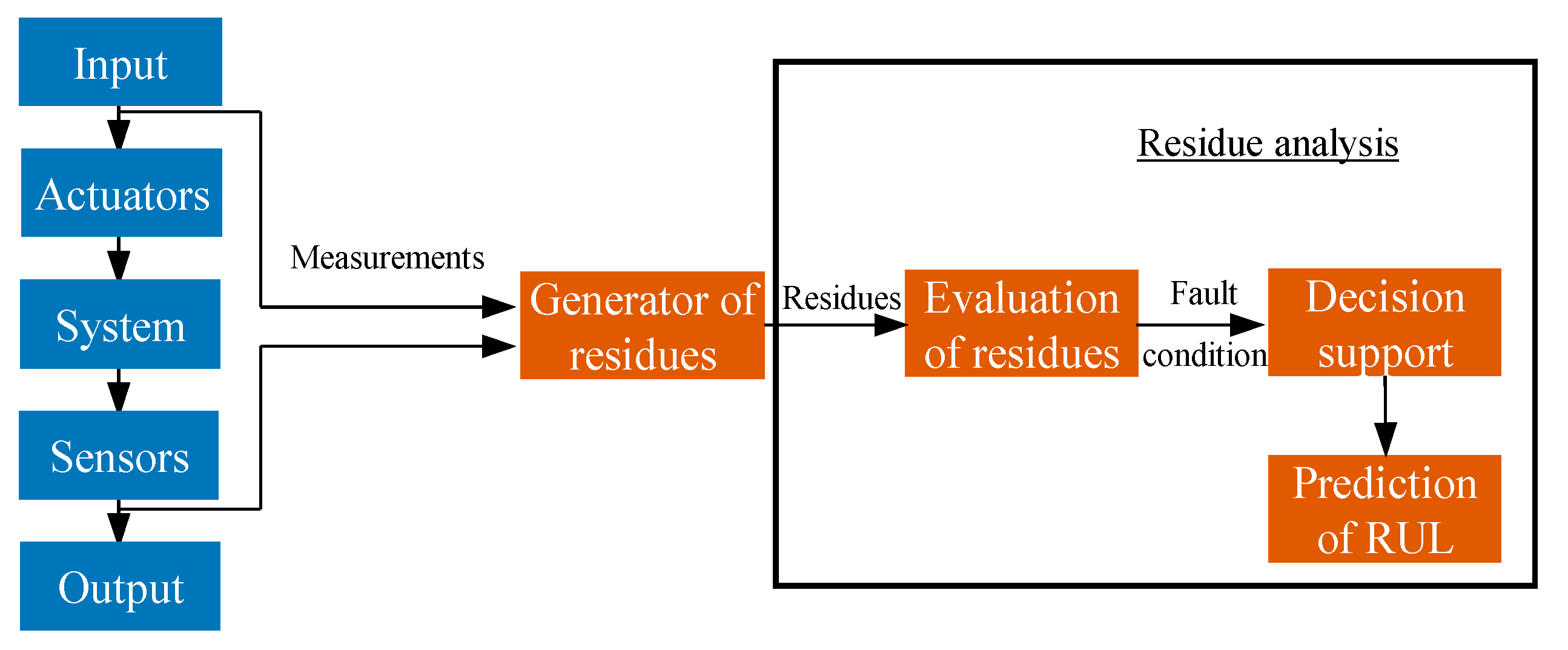
Model-based prognosis deals with a physical model that uses mathematical representations to include a physical comprehension of the degradation process [11]. A conceptual diagram of the model-based prognostic is displayed in Figure 5. It consists of investigating the physics of the monitored system’s failure and representing it by a physical model [21]. Mathematical functions, such as differential equations, are developed to represent the system [22]. These equations are then used in statistical techniques such as Kalman filters and parity relationships to evaluate the system’s state. Residues that are the difference between the model prediction and observations are then used to detect, isolate and predict the system’s degradation [11]. Residues show the divergence between the system model and actual observations. The statistical analysis of these residues allows for detecting degradation in which the prediction is performed to estimate the remaining time until the occurrence of a fault by setting a predetermined default threshold.

Figure 5.
Typical architecture of model-based prognostic methods.
The first benefit of this approach is that it does not require the historical data to estimate the future state of the system when the model is known. Another benefit is that it allows for considering the deterioration caused by environmental conditions such as heat, humidity, vibration, loads and shock. However, its drawback is that a mathematical representation of a system requires a deep understanding of the subjacent physical processes that lead to system failure [22]. It is also necessary to define a physical model for each mode of failure as well as the data describing the conditions related to each process [23]. The creation of models representing the different physical processes produced is also a difficulty to overcome [11].
2.1.1. Physics of Failure
The implementation of a model based on the physics of failure (PoF) is valid in the absence of observations and the availability of observations only. It considers the physics of the system, the system’s degradation behavior as well as failure modes and uses the degradation properties such as material, geometry and loading conditions [23]. Thus, this method identifies degradation trends and estimates the RUL [24]. A typical PoF model is the fault propagation models such as spalls propagation or cracks. Lie et al. [25,26] established the relationship between bearing defect growth rates, defect zone size and material parameters through the crack propagation modeling technique. This method is based on Paris’ Law crack growth where a least-square scheme allows for adaptability to changes in the system state. However, the material parameters have to be determined in an empirical way, and the defect area size is considered linearly correlated to vibration root mean square level. Furthermore, this approach was also used in [27,28] but with the addition of a 2D finite element analysis that calculates stress and strain based on the load of the gear tooth, the defect size, geometry and material properties. However, this method needs high computation capacity. In [29], another PoF based on the propagation model is the Forman law crack growth used for rotor shaft crack growth, which has to link condition monitoring information and crack physics to life models. The Yu–Harris equation for estimating bearing life, with a stochastic version, has been exploited by [30,31] in order to forecast spall beginning. These authors also used the Kotzalas–Harris progression model to assess the time to failure. This framework was enhanced in [32]. The Contact Analysis for Bearing Prognostics program (CABPro) was used in [33] using finite element analysis in order to calculate material stress based on defect dimensions, bearing geometry, load and speed. After this step, the cycles to failure are estimated. Furthermore, acceleration amplitude and natural frequency of a rolling-element bearing were used to determine the failure time by taking the element as a vibratory system with only one degree of freedom [34].
2.1.2. Bayesian Estimation with Kalman Filters
Kalman Filter (KF) is used as a model for approximating system output based on a certain gain. The difference between the estimation and the actual output is used to generate residuals that are used for diagnostic and prognostic purposes. It is designed for linear systems through minimization of the squared error between the input without noise and the one with added noise. It considers that additive measurement and process noises are independent and Gaussian. When non-linear systems or links between systems and measurement take place, KF is replaced by Extended Kalman Filter (EKF), which proceeds by partial derivatives to linearize the estimation. Recently, EKF was used in [35] for prognostic of the proton exchange membrane fuel cell. However, when noise is not Gaussian, EKF is no longer reliable because calculation time will increase and cause the divergence of the filter when calculating the Jacobian matrix [36]. Other forms of enhancements for non-linear systems with Gaussian noise exist and are different from one another in terms of the method used for integral estimation. Such enhancements are the Gauss–Hermite Quadrature Kalman Filter as well as the Unscented Kalman Filter, which is an extension of the Quadrature Kalman Filter and Monte-Carlo Kalman Filter [37].
2.1.3. Bayesian Estimation with Particle Filters
Sequential Monte Carlo methods are particle filters that are used to estimate an online future state and alleviate the drawbacks of KF and its derivatives. The concept of this filter is to use a set of random samples called particles, iteratively generated to represent the posterior Probability Density Function (PDF). They are associated with weights that are updated with each generation. Thus, the outputs estimates are calculated according to these particles and their weights. Moreover, particles of dynamic noise are also drawn at each iteration. The higher the number of particles, the nearer the filter output is to the posterior Probability Density Function (PDF). However, when the number of iterations increases, the posterior PDF approximation tends toward zero [38]. It is possible to attenuate this effect by increasing the number of particles but it is not always applicable. Hence, at the end of each iteration, a resampling step must be added. Recently, particle filtering approaches were thoroughly developed, and the results showed that Unscented Kalman filter is more accurate and has less calculation cost than particle filtering [39]. The authors in [40] used a particle filtering framework for lithium-ion battery health management prognostic [41] and Miao et al. used an UKF for the same purpose [42].
2.2. Data-Driven Prognostic
The remaining useful life is estimated by the data-based prognostic approach when the system in question does not have a reliable model. The RUL predicts the time before the defect exceeds some predetermined alarm value.
Data-driven prognosis hypothesizes that the monitoring data are stable until a fault occurs. In the data-driven prognostic approach, indicators represent the degradation of the system. In the first step, sensitive indicators are extracted from the data thoroughly after an analysis phase. In the second step, prediction methods are used to study the evolution of these indicators and their trend in order to estimate the time remaining before the failure worsens the system and exceeds its previously set threshold value [20]. Figure 6 summarizes the data-driven prognostic structure. A new risk assessment framework that includes PHM and PRA (Probabilistic Risk Assessment) techniques and concepts were presented in [43]. In this work, the authors presented a hybrid model, which combines both PHM and PRA concepts, to deliver a forward-looking approach to risk assessment to study complex engineering systems.

Figure 6.
Architecture of a data-driven prognosis.
Data-driven prognosis offers many advantages compared to the model-based one. It learns the system behavior based on data provided by sensors and therefore does not require any specific knowledge for modeling purposes. Furthermore, the number of extracted features is large if it is a complex system, and this technique could be successfully applied. Data-driven prognostic methods categorization is given by [16,19,44].
2.2.1. Knowledge Based Models
In order to determine the RUL, the so-called knowledge-based methods compare and estimate the similarity between the real situation and a dataset including the failure. They regroup expert systems and fuzzy-rule based systems.
Researchers have applied expert systems to solve prognostic problems. This involves using a set of syntactic rules and if-then statements, combined with knowledge gathered from experts to determine how and when this knowledge should be applied. This development allows to provide the expert system in the form of a software [45]. The latter is updated in a continuous way according to the changes of the system configuration. Furthermore, a set of inputs in the database provides an output, and as the number of inputs/outputs expands, the number of possible combinations may generate a combinatorial explosion [46].
The use of fuzzy rule-based systems allows for the remediation of the disadvantages of expert systems. These fuzzy systems are not sensitive to noise and require fewer rules and work correctly even if the data are incomplete. However, these fuzzy approaches, which are based on probabilistic models, use an approximate rule set instead of exact rules [47]. Fuzzy logic has been developed to handle the concept of partial truth, where the truth value can range between completely true and completely false. Thus, the decision making is replaced by fuzzy sets, and the rules are replaced by fuzzy rules. This method seems to be efficient when handling noisy and inaccurate data because it works in an intuitive way.
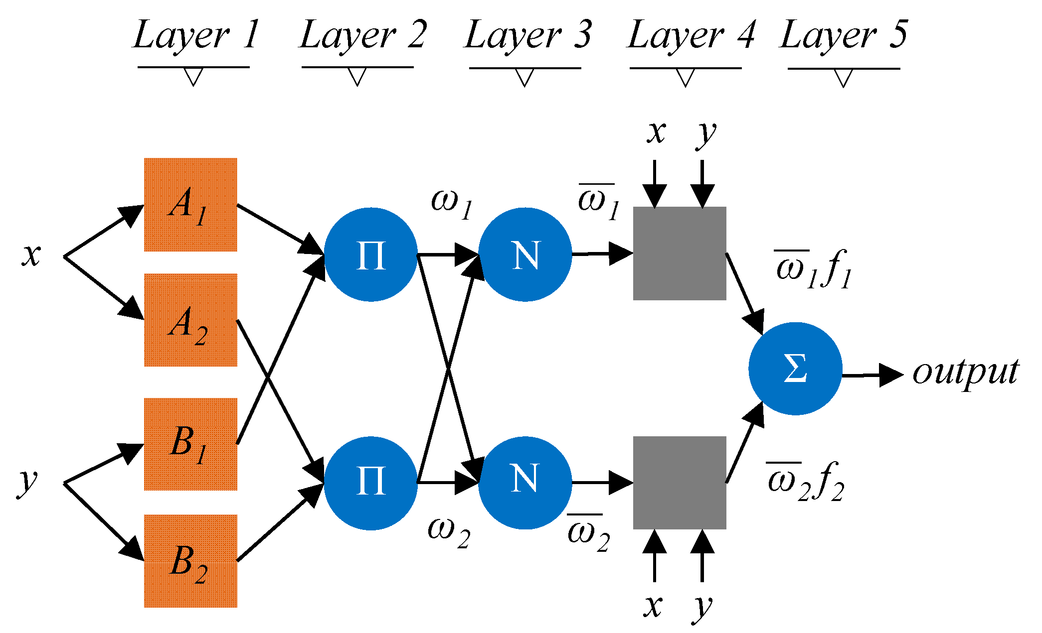
The fuzzy logic becomes more complicated with complex systems due to the large number of rules. In this case, the neural-fuzzy (BF) method allows to simplify it. This last one includes both neural networks and fuzzy logic principles. The combination of the two approaches allows one to avoid the problems that are related to the distribution of the membership function of the fuzzy logic and how to choose its nature, including how to compose the fuzzy rules and how to overcome the problem of incomplete knowledge [48]. For example, the neuro-fuzzy inference system is described by a black box that contains the set of fuzzy rules that weigh the inputs and provide a single output [49]. As shown in Figure 7, the ANFIS structure is composed of five layers: fuzzyfication, weighting, normalization, defuzzyfication, and summation [50].

Figure 7.
ANFIS architecture for two inputs and two rules.
Each input (x, y) is linked to membership functions (A1,2, B1,2) that evaluate their degree of membership. The membership functions are associated with fuzzy rules via weights noted ω1,2. In layer 3, each weight is normalized, and a set of (IF-THEN) rules is computed. The output of the ANFIS system is given by the sum of the contributions of all the rules able to approximate non-linear functions [51]. In [52], a study comparing techniques (ANN, ANFIS) and a new method called Coactive Adaptive Neuro-Fuzzy Inference System is realized. It combines an extended form of the ANFIS, which manages any number of input–output pair and a Genetic Algorithm (GA). GA optimizes the system’s performance and overcomes some problems of the ANN such as optimizing the network parameters including learning rate and the momentum of the network for each input. This study estimates the ore grade and shows that CANFIS-GA is more accurate than non-optimized techniques.
In [53], the authors implemented the ANFIS method for the prediction of skin temperature in lower membrane prostheses. Then, they compared it with Gaussian process machine learning methods. The results show a similarity in terms of performance between the predicted and real data. This technique can be used for the invasive monitoring of temperature.
2.2.2. Life Expectancy Models
The degradation of the process behaves like a stochastic process influenced by random sources due to variability and uncertainty of processes. Therefore, stochastic models are used to complete prognostics [9]. Several stochastic and statistic models have been used to model the system degradation process [54,55,56].
Stochastic Models
When the system is complex, building a physical model is complicated. In such a way, the idea is to bulify an experience approach, which is based on the stochastic modeling of the degradation based on a collected dataset. These models consider that the times to failure of identical systems are statistically the same and follow a random distribution. Therefore, they are represented by a function of probability density.
- Aggregate reliability functions
The industrialists have given a lot of interest to the reliability analysis approach of aggregated failure data for predicting the system state [55]. The approach consists in estimating the probability density function by analyzing the failure times of a set of components [57]. The phenomenon of degradation is modeled in various distributions, but when it is gradual, it is more convenient to use the Gaussian function [58]. The Weibull distribution is often used in the field of life analysis, due to its flexibility: as said before, it allows for one to represent at least approximately an infinity of probability laws. This function is subject to all types of degradation and is used in prognosis. Its strong point lies in the fact that it does not require a detailed knowledge of the physical mechanism and the degradation [59]. An algorithm was proposed to automatically calculate the parameters of the Weibull distribution from a machine database of downtime [60].
- 2.
- Conditional probability model
The objective of the prognosis is to estimate the time to failure or residual life as well as the risk of existence or subsequent occurrence of one or more failure modes. To estimate this duration, a probabilistic model based on Bayes’ theorem could be used. A reliability function is used to present the actual state, and then, Bayes’ theorem is applied to evaluate the probable values of the future behavior [61].
The probability density function of the components is necessary to generalize the classical reliability study and to represent the probability density function of the remaining useful life. It is assumed that the observations are added later as predictive density functions and that the equipment distribution is updated by Bayes’ rules. In this case, Bayesian networks and Kalman filtering approaches can be used to improve the prediction process that depends on the system and noise type. Moreover, in most cases, this process is not simple since it requires integral resolution. Thus, several methods based on approximation to estimate integrals were used, such as regression models [62]. The accuracy of the method is inversely proportional to the remaining useful lifetime (RUL). As the RUL increases, the accuracy decreases and vice versa.
Furthermore, the Static Bayesian Network (SBN) is a directed acyclic graphical model composed of random variables and their interdependent probabilities [63]. The variables are represented by nodes that are characterized by a conditional probability table depending on the predecessor’s states [64]. In Bayesian network theory jargon, the term “vertex” is commonly replaced by the term “node”. These networks model the evolution of the state of a component as a function of influencing factors, where the arcs of the graph represent the probable causality between two variables. This probable causality will be quantified by a conditional probability. Bayesian inference is easily performed and with a low computational cost due to the graph theory.
The implementation of a Bayesian network requires two x major phases. The first one is used to construct the graph, i.e., to identify the variables of the variables of the model and to indicate the dependencies and conditional independence between these variables. The second phase consists in calculating or evaluating the probabilities needed to calculate the joint probability of all the variables. These two phases can be performed either by a model selection procedure with feedback data, by expert opinion, or by a combination of both. Despite the complexity of this approach, it is useful when the database is incomplete. Moreover, it is adaptive to new observations but may have a high computation time.
The authors in [65] have developed an adaptive Bayesian decision model in order to assess the more convenient periodicity of replacement and examination parts. Moreover, a novel approach called objected-oriented Bayesian networks was proposed to predict the system’s state in the future by one step forward time series forecasting [66]. This work does not include RUL estimation but proved the consistency of SBN when used for prognostic purposes. In [67], the authors developed a Bayesian framework that exploits actual condition monitoring observations to update the stochastic parameters of exponential degradation models. When the degradation signals are well modeled, they characterize the residual-life distribution of the system. In [68], a degradation model was developed for the study of rotating bearings monitoring systems. This model was carried out in two stages and is combined of two parts, a part that follows a linear function and a random part simulating the errors. The degradation rate passes through a switching point where the rate takes different values before and after this point, which allows for a two-stage degradation model. The degradation level and time represent the switching points. This model remains limited because it is based on a linear regression. In addition, Bouaziz et al. [69] developed a Bayesian network methodology based on a predictive model. This methodology is used to predict the system health factor applied on complex semiconductor systems. The same idea was developed recently by Bian et al. in [70], who used a Bayesian framework to update a signal and conditions parameters as well as the residual lifetime distribution of the monitored system.
Dynamic Bayesian Networks (DBN) also exist, which are Bayesian networks that relate variables to each other over adjacent time steps. Among DBN, the Markov Model (MM) is a stochastic model that is used to model randomly changing systems where it is assumed that future states depend only on the current state, not on the events that occurred before it and that the state is visible to the observer [71].
The time horizon of contracts is an important criterion that must be considered during the coordination process. This consideration simply considers the aging process that the assets will undergo and not only the amortization of the investments made by the providers. The authors in [72] present a range of methods such as the Semi-Markov model (SMM) or the Semi-Markov model (SMM). They consider the repair and replacement of critical components. The proposed methods are adaptable for RUL estimation. In [73], Carlin and Chib estimated the Remaining Useful Lifetime by the Monte-Carlo hazard model.
The drawback of MM and SMM represents their inflexibility to temporal failure degradation, which means that they cannot consider gradual failure and are not applicable to partially repaired systems. In general, the degradation of the failure is gradual, which limits the use of Markov and semi-Markov models. To remedy this, hidden Markov models (HMM) have been developed, but their learning requires a large database and powerful computing unit. As shown in Figure 8, two parameters are used to describe this, defined by two parameters, to know the model states’ number and the different observation symbols per state’s number . In addition, three probability distributions are important, namely the state transition probability distribution (), the observation symbol probability distribution and the initial state distribution [74].
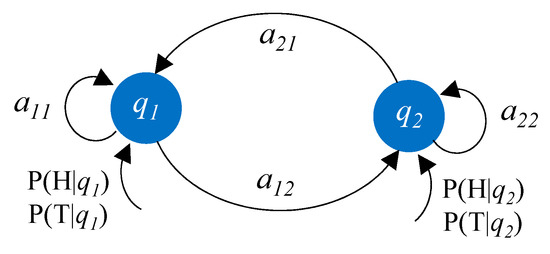
Figure 8.
HMM with the states q1 and q2, the output alphabet {H, T} and the transitions and output probabilities as labeled.
This method has been used in several domains, but it has been applied to the prognostic. As the authors note in [75], a precondition for the successful implementation of CBM practices in the industry is efficient diagnosis and prognosis. In their work, they describe a method in which several HMMs are used to represent the health status of a metal cutting tool and to evaluate the RUL of tools.
The Hidden Semi-Markov model is used to predict the RUL. This model is similar to the Hidden Markov model. The difference between the two lies in the probability of state change that remains fixed in the HMM and that depends on the time elapsed between the beginning and the current state for the HSMM. In [76], the authors developed a new approach based on segmental SHMM that combines the diagnostic and prognostic operations. The developed approach allows for predicting the RUL. Moreover, this approach facilitates the computation and uses a novel forward–backward algorithm for the training of HSMM. In [77], two algorithms based on SHMM were used to forecast a future state; thus, they provide the RUL estimation of a complex system as a function of time. Recently, R. Moghanddass et al. in [78] introduced a non-homogeneous semi-Markov model to discuss the parameters’ estimation for the model’s training and to develop the measures of the prognostic model reliability including the mean residual life. This model takes into account that the system exhibits several degradation states under limited observations during the operation of the monitored system. The model was applied to a bearing shell to monitor its degradation and to demonstrate the model’s validity. HMM and SHMM have better adaptability to gradual failures, but they are reliable for fault prediction only when a sufficient amount of data covering all progression stages of the failure are provided [19]. In addition, all MM need a large capacity of calculations depending on the model complexity. Thus, they have been often combined with a dimensionality reduction method (PCA) [79].
Another stochastic model is the rain flow counting method [80]. This is based on counting stress-reversal fatigue cycles from a time history by the application of Miner’s rule (a cumulative damage model for fatigue produced failures) for the assessment of fatigue life of a complex-loaded structure. This method allows for transition cycles to be processed accurately but does not fully account for the slowly varying mean stress [81].
In addition, the first/second-order reliability method (FORM/SORM) is a reliable method for structural prognosis [35,82]. In FORM, the reliability index is seen as the minimum distance between the origin and the limit state surface, and its design point (the most probable point of failure) is then searched. However, there is an accuracy problem when the performance function is non-linear. SORM is, in consequence, introduced as a solution, and it is obtained by approximating the limit state surface by a second-order surface [83].
Statistical Models
Statistical models go through two steps, which are evaluation and prediction. The first step consists in evaluating the evolution of faults by considering historical data of a system. The second step allows for extrapolation of the data to predict the future state of the system.
- 3.
- Trend evaluation
This method consists in using a parameter calculated from the data acquired by the sensors. This parameter is well correlated with the RUL and will be followed over time. The implementation of an alarm and a pre-alarm determines an estimate of the RUL. Once the trend is established, extrapolation regression methods will be used to predict the RUL and to track the progression of degradation over time. This method is limited by the noise that comes from different sources putting uncertainty on the results obtained (see Figure 9). To remedy this, advanced techniques can be used to model the noise and take it into account in the estimates [84].
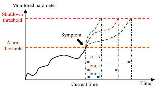
Figure 9.
Illustration of RUL with uncertainties [84].
- 4.
- Autoregressive models
An autoregressive model (AR) is a linear predictive modeling technique used to predict the evolution of a monitored parameter on the basis of previous observations by using the AR parameters as coefficients. Many regression methods were used for RUL forecasting such as the autoregressive moving average. The autoregressive moving average was applied for stationary signals. This model is able to model uncorrelated time series, and it is applicable for prognostics [85,86,87,88,89]. For non-stationary signals, the Autoregressive Integrated Moving Average Model (ARIMA) gives better results in the case of noises in the observations. It deals with the observation values as well as the noises in the observations and thus yields minimal modeling error [90].
Recently, authors have presented in [91] a method to estimate the health status of the system and to predict its reliability in evolving trends in an online condition monitoring applied to a vertical roller mill. This method uses the integrated moving average model presented before and forecasts the state of the parameters, which is the input of a multi-observation HMM. The parameters of the AR model are estimated by non-linear optimization techniques method in order to minimize the estimation error. Finally, the model is validated through the examination of standardized residuals and the autocorrelation of residuals [85].
The shortcoming of this method is its inefficiency when the historical data are incomplete, which may lead to a false extrapolation [92]. Furthermore, these models are less efficient for long-term prediction because of the dynamic noise. This is reduced by exploiting predictions based on actual observations for RUL prediction instead of past predictions [88].
2.2.3. AI Approach
Recently, many data-driven methods of prognostic systems have been implemented based on the Artificial Neural Network (ANN) approach because of its good efficiency in the field of state prediction and direct RUL estimation. The learning capacity of ANNs from the system historical data make them the most common tool of system prognostics. The values of an ANN’s input layer are successively weighted and processed by artificial neurons of the hidden layers, which simulate the biological neuron concept to obtain one or multiple estimation values at the output layer [42]. ANNs are faster than traditional statistical prognostic methods [92]. Furthermore, they are more reliable for complex non-linear systems that do not need a considerable amount of data.
Several papers reporting the use of long short-term memory (LSTM) networks for RUL are studied in the literature. We can cite the work of Liu ZH and all the authors in [93] who applied an advanced approach combining an elastic net long short-term memory network (LSTM), with the aim of increasing the predictive accuracy of the remaining useful life (RUL) of the rotating bearing in rotating machinery. Another approach, based on the deep learning model using LSTM autoencoders, is employed for predictive maintenance in cyber-physical production systems [94]. A variant of the LSTM approach, called the convolution-based long short-term memory (CLSTM) network, is proposed to predict the RUL of rotating machineries mining the in situ vibration data [95].
An adaptive prognostic method was proposed and applied to lithium-ion batteries to forecast their end of discharge by training online the radial basis (RB) function model [96]. In [97], Tian et al. proposed a prognostic approach of a wind power generation system using a feed-forward neural network model with two hidden layers. The inputs of the ANN model were the component age and the condition monitoring measurements at the inspection points, and the output was the life percentage at the current inspection point.
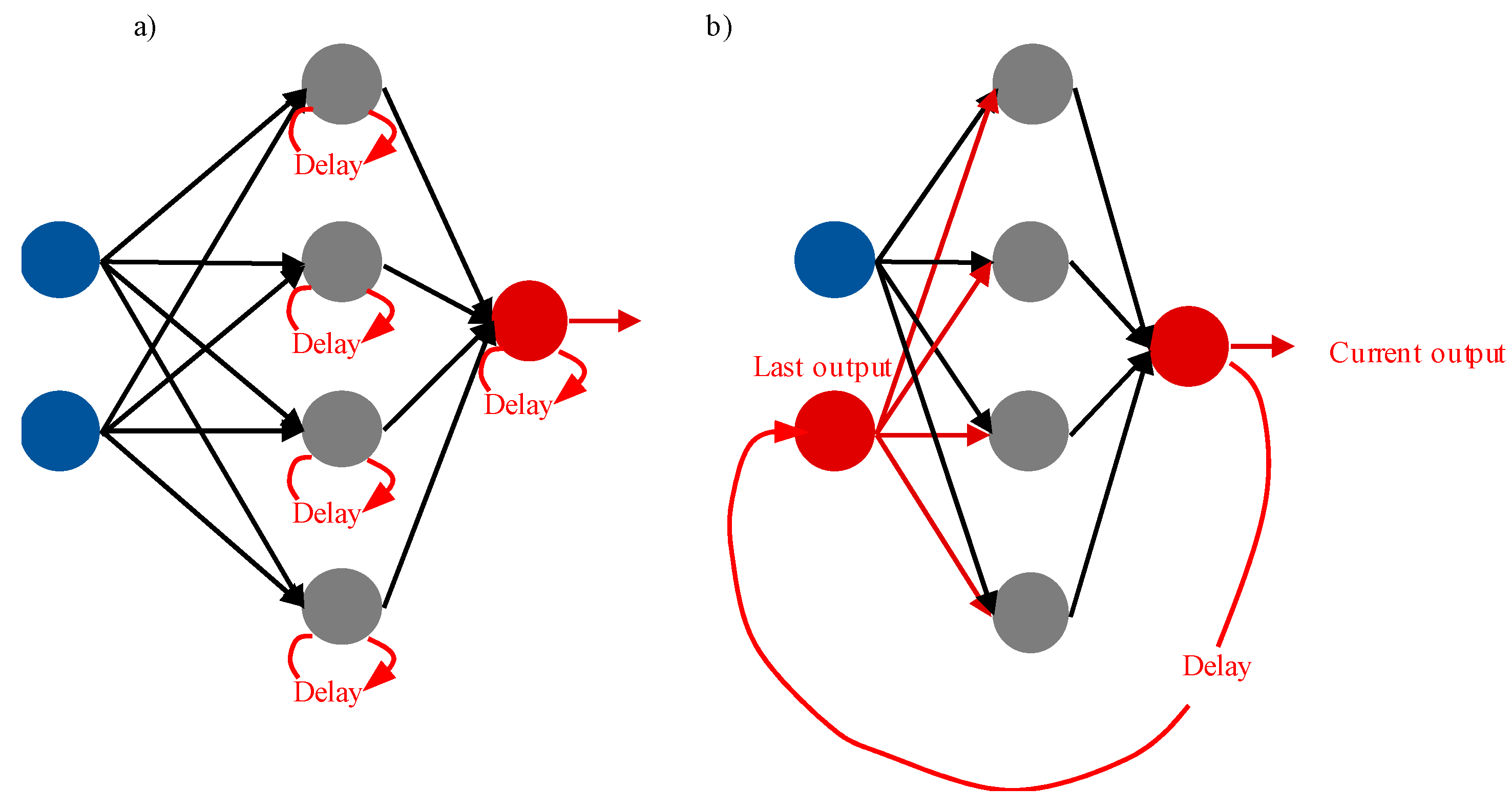
ANNs are reinforced when combined with different techniques. For instance, hybrid neural networks that can accept different types of inputs were introduced by Wang and Vachtsevanos [98]. In addition, Wavelet Neural Networks (WNNs) were used for failure assessment based on their features. Dynamic Wavelet Neural Networks (DWNNs) were also used to forecast the fault evolution and to assess the RUL. In [99], Yam et al. used recurrent neural networks (RNNs) to build an intelligent predictive decision support system for power plants’ integrated maintenance management. RNNs are obtained by adding a temporal memory to the network using the past internal state of each node [100,101]. Moreover, Time Delay Neural Networks (TDNNs) are another dynamic architecture of neural networks commonly used for time series prediction [102]. As seen in Figure 10, TDNNs and RNNs work in a sequential way; thus, they are called feedback neural networks, which make them more convenient for prediction applications since they are time variant.
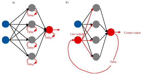
Figure 10.
Typical architectures of (a) RNN (b) TDNN [101].
Decision-making support is the ultimate mission of predictive maintenance; it consists of scheduling the best maintenance interventions at the right time using the RUL prediction outcomes [103,104]. The authors in [105] used the self-organizing maps (SOMs) or Kohonen map, where an automatic fault mode detection is presented based on the SOM network and the kernel density estimation with as little as possible prior knowledge.
2.2.4. Deep Learning Approach
More recently, machine learning, particularly deep learning methods, has gained popularity in the field of PHM. Many studies have examined how deep learning can improve the overall performance of PHM [106,107,108].
Deep Learning (DL) algorithms have recently emerged in the field of prognosis. Since then, several algorithms have been introduced and are used in various application areas.
Today, the use of DL has become essential due to their intelligence, efficient learning, accuracy and robustness in building prediction models [109]. In the literature, the most recently used DL algorithms can be classified into tree main categories: Convolutional Neural Networks (CNN), Deep Belief Neural Networks (DBN), and long short-term memory networks (LSTM).
Convolutional Neural Network (CNN)
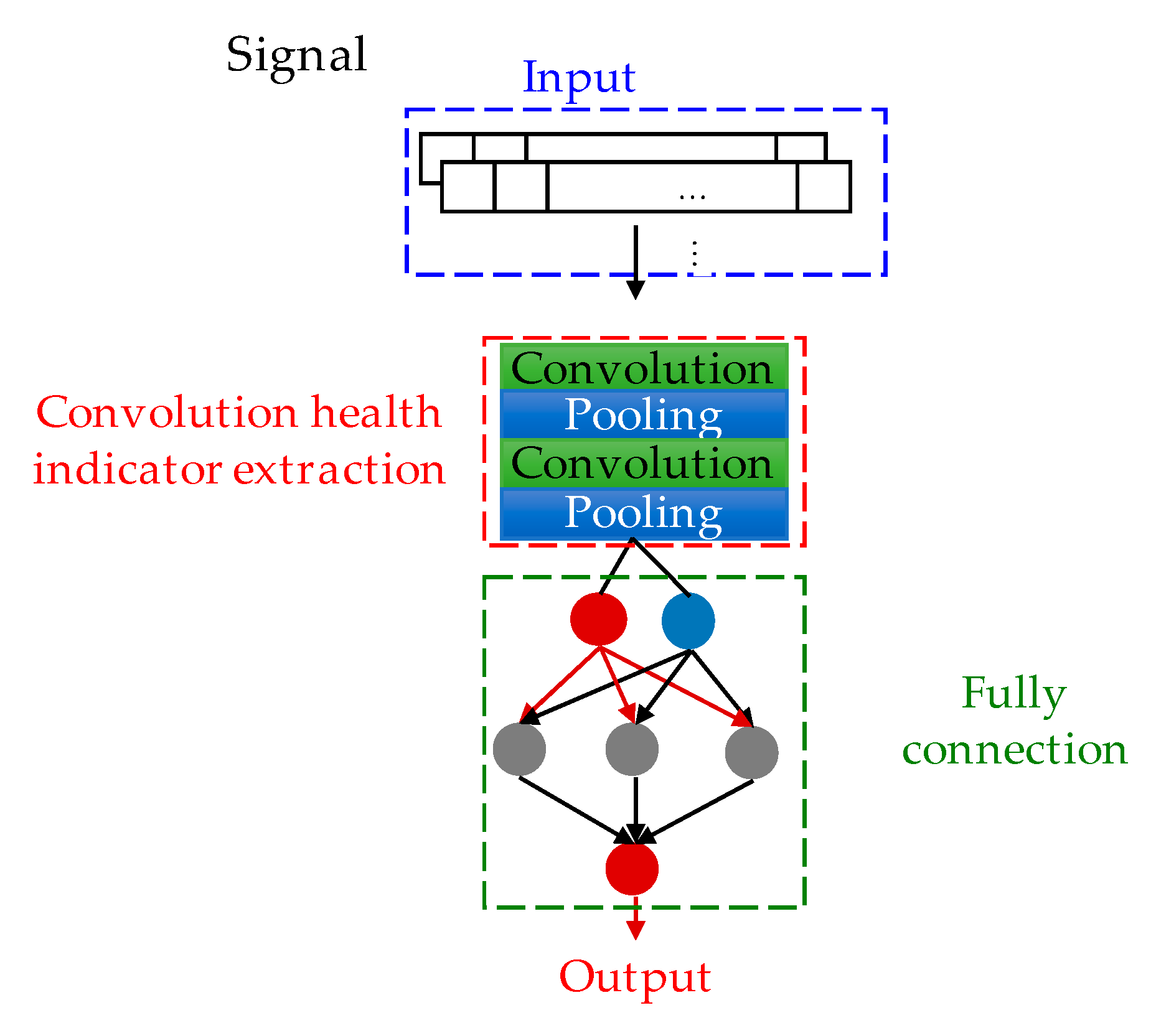
CNN is one of the best-known architectures of Deep Learning techniques. It has been proposed for fault prediction in flight vehicle systems [110]. This technique starts with raw sensor data; learns sensor dependent features and timing features through convolutional layers; and predicts the remaining useful life of aircraft components. This technique can be used in other field fields such as bearings and machining processing [111,112]. CNN contains three types of layers with different convolutional, pooling and fully connected layers. In each CNN, there are two steps for the learning process, the feedforward step and the backward step. In the forward step, the CNN takes a set of nodes and transforms it into a convolutional layer with filters or Local Receptive Fields considering the overlap window. After activating these transformations using the predetermined activation function, the new data space will again be down-sampled (pooled) using a well-defined sampling type such as (mean, min or maximum). The convolutional layers and the down sampling layers are locally connected. The final down-sampling results will be fully connected to the output layer. In the backward step, the learning algorithms will try to tune these connections (weights) based on the approximation error to satisfy the target function. Generally, CNNs are trained using the back-propagation algorithm. Figure 11 illustrates the fundamental architecture of a CNN neural network.
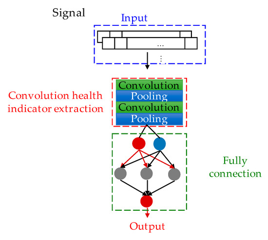
Figure 11.
Architecture of a CNN.
Deep Belief Neural Networks (DBN)
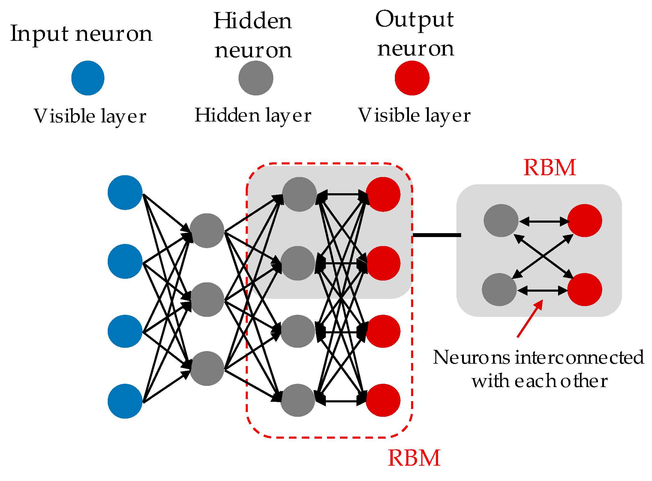
DBN are probabilistic generative models composed of several visible and hidden layers of stochastic latent variables. Hidden layer variables are typically binary, while visible layer variables can be binary or real. The two upper layers are the restricted Boltzman machine (RBM). RBM in its restricted version consists of two layers: a layer with input neurons, and a layer with hidden neurons. All of these neurons are interconnected. Much like autoencoder networks, the hidden layer often has fewer dimensions than the visible layer (although this is not always the case). To illustrate the concept, Figure 12 shows a diagram of a restricted Boltzmann machine. As can be seen, we only have two layers and all the neurons are interconnected with each other. Unlike conventional neural networks, information no longer flows from the input layer to an output layer. We are here in a logic where information circulates in a circular way. In its initial design, the algorithm is used to study the relationships between inputs and outputs.
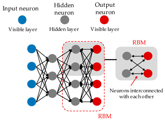
Figure 12.
DBN architecture.
DBN can be considered as a composition of simple networks and unsupervised architectures such as restricted Boltzmann machines (RBM). The deep belief network consists of an RBM layer for pre-training and a feedforward neural network for the fine-tuning phase. J. Deutsch et al. in [113] used DBN trained with data collected from bearing profiles to predict remaining life in higher-dimensional space. The advantage of using DBN is that it only depends on a small training set to achieve good tuning of unsupervised and supervised parameters. J. Ma et al. [114] used auto-encoders based on “Sparse Coding” combined with a hidden layer of logistic output for learning a DBN for the prediction of the RUL of aircraft engines. DBN are considered as very intelligent prediction methods and are available for a variety of applications.
The Long Short-Term Memory Networks (LSTM)
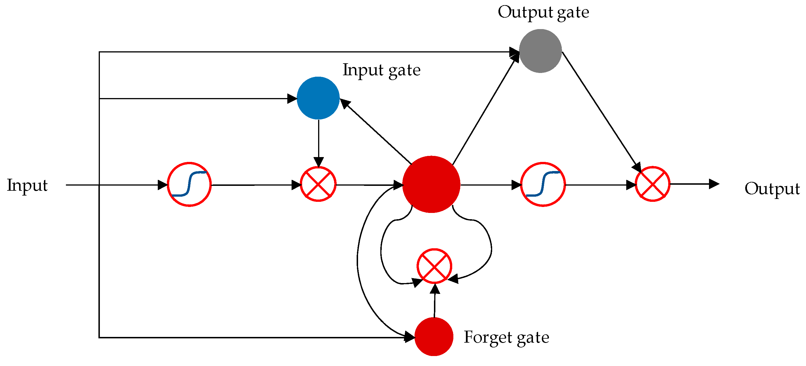
Traditional RNN have a limitation in learning and encounter the problem of vanish gradient problem if the time series is too long. Moreover, RNN are only able to memorize the so-called near past and begin to “forget” after about fifty iterations. The long short-term memory networks make it possible to bypass this lock. A LSTM unit is composed of a cell, a forget gate, an input gate and an output gate that manages a dynamic memory (denoted C), which evolves according to the temporal data sequence, this architecture is illustrated in Figure 13.The Forget Gate is an operation leading to the ability to forget information (or to greatly reduce its weight), which was useful at time t − 1 but which is no longer so at time t. Input Gate is, on the contrary, an operation that gives the cell the ability to store new information at time t while this same information is non-existent or of little relevance (very low weight) at time t − 1. Finally, the output Gate controls the information that will be transmitted at time t + 1 according to the memory C and the activation function. The LSTM cell, due to this memory vector C, stores the values over arbitrary time intervals, and the three gates regulate the flow of information into and out of the cell.

Figure 13.
LSTM architecture.
Z. H. Liu et al. in [93] proposed the LSTM method to forecast the RUL of rolling bearings. The algorithm is called E-LSTM, and it consists of an elastic mesh and LSTM, taking temporal–spatial correlation into consideration to forecast the RUL through the LSTM. In [115], LSTM neural networks were used to solve the bottleneck problem of high-precision RUL estimation for complicated engineered systems.
2.2.5. Similarity-Based Learning
Similarity-based methods mainly aim to build an offline equivalent model of the system degradation behavior using supervised machine learning techniques. Regression is a well-reputed technique in this domain due to its good results in prediction and forecasting applications [92]. Many algorithms such as k-Nearest Neighbors and belief functions were used to assess the system health and then estimate its RUL. It was applied in [116] for turbofan engines when a degradation attains a fixed threshold.
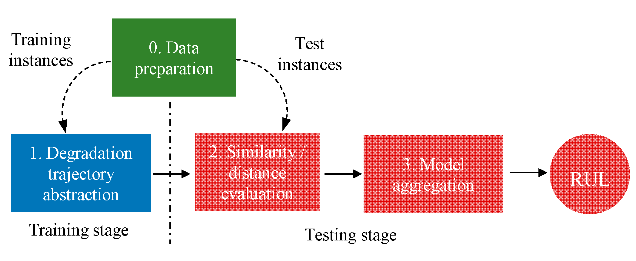
Tianyi Wang proposed an alternative learning methodology for the RUL prediction of a turbofan engine called Trajectory Similarity Based Prediction (TSBP) in [90], where a library of degradation models was created based on historical condition monitoring data and failure times. Then, these RUL estimates of the different degradation models are aggregated with a density estimation method to obtain the final RUL estimate of the test instance. This model aggregation was also presented by Eker et al. in [117], as shown in Figure 14.

Figure 14.
Typical procedure of TSBP approach [117].
In [118], Ramasso et al. proposed a new similarity-based prognostic approach called EVIPRO-KNN, where belief functions were used to deal with the lack of data labels and to manage degradation trajectories with different temporal lengths. In addition, the developed model was applied to predict jointly continuous and discrete states of the system degradation. When expert knowledge is available, the fuzzy-based similarity can be carried out to assess the distance between run to failure information by using fuzzy membership functions instead of sharp distance consideration [119].
2.3. Hybrid Prognostics
As shown in Figure 15, this approach revolves around the combination of model-based and data-driven methods in order to benefit from their strengths [17]. These methods tend to simplify the physical model when the monitored system is more complex. They are divided into two categories: series approach and parallel approaches [17].
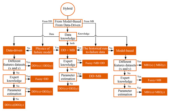
Figure 15.
Scheme of hybrid methods-based prognostic.
The series approach, as shown in Figure 16, is based on extracting parameters indicating fault evolution from sensor output signals. Then, certain model parameters will be reassessed according to these signals such as recursive estimators. Hence, the output of the first method is fed into the second method. This approach is used in real-time prognostics. It includes four combinations: data-driven + data-driven, data-driven + model-based, model-based + data-driven and model-based + model-based methods.

Figure 16.
Series approach structure.
In the parallel approach illustrated in Figure 17, data-driven methods are used to complement model-based methods when they are incapable of modeling certain processes. Then, in order to perform the prediction, the residues are gathered and used from both methods. This approach enhances the prognosis accuracy. The combination of the outputs of model-based and data-driven approaches is achieved by fusion techniques such as fuzzy fusion or statistics-based fusion. This approach includes two combinations: data-driven/model-based and model-based/data-driven methods.

Figure 17.
Parallel approach structure.
Creating a hybrid prognostic application is achieved by carrying out hybrid methods upfront or associating already realized data-driven or model-based methods to other methods.
2.3.1. Data-Driven Combinations
If the previously implemented approach is data driven (DD) and the physics of failure are unknown, it is more convenient to carry out DD combinations to enhance the results accuracy. When the data present various scenarios, the same DD method is applied to each scenario in a parallel structure based on DD combination. It was applied to enhance the prediction performance for a nuclear power plant with a modified probabilistic support regression [22]. Moreover, when expert knowledge is available, it is associated with the DD method, which was applied in [120]. In this paper, the authors used expert knowledge as fuzzy logic and associated HMM to the adaptive neuro-fuzzy inference system. However, when expert knowledge is not available, a DD method is used as a parameter estimator and the other DD method put into the series gives more accuracy. This was the case in [121] where Liu et al. used the least square support vector regression with HMM in order to predict the future faults and the RUL. If all these tests are negative, DD methods are merged in parallel as in the case in [122] where Hu et al. combined multiple number algorithms with a weighted-sum formulation. These weights are determined by three proposed weighting schemes. This approach forecasts future faults and assesses the RUL.
2.3.2. Data-Driven and Model-Based Combinations
DD and MB methods can be combined to enhance their performance. When expert knowledge is available, it is combined with DD and MB methods. For instance, fuzzy logic is used with the DD method to enhance parameter estimation, which will be the input of the MB method. In the case where there is no expert knowledge, DD and MB methods are combined to estimate the prior parameters of the MB method by the DD method. In [123], a hybrid approach for RUL estimation was proposed, which consists of combining neural networks and based particle filtering. MB and DD are combined in a parallel way to enhance RUL estimation accuracy when the conditions are not verified. This model was built in [124] by using an ensemble of Kernel regression with PoF models. Recently, a framework for a hybrid model for RUL prediction was developed in [125]. The proposed method is able to enhance forecasting accuracy and consists of combining two DD methods with a particle filter. The first DD method estimates the measurement model, which is a mapping from measurements to system state while the second DD provides a prediction of future measurements in order to decrease the uncertainty of the long-term prediction of the particle filter. The flow chart of the proposed method is shown in Figure 18.

Figure 18.
Fusion of data-driven and model-based methods [125], Reprinted with permission from Elsevier: license number 5387500327402, 14 September 2022.
2.3.3. Model-Based Combinations
When knowledge contains various scenarios, MB methods are combined in a parallel manner, as is shown in [126]. An ensemble of empirical models gives the RUL estimation of each model, and they represent the input of the Kalman filter-based algorithm. This method was applied to turbine blades undergoing developing creep. Moreover, when expert knowledge is available, it is associated with the MB method in order to control uncertainties. It was applied in [127] where multi-sensor data fusion based on fault detection and fuzzy Kalman filter feedback were used to reduce vehicle risk. When there is no expert knowledge, BM methods are used in a parallel manner to estimate parameters such as in [128] where UKF is used to estimate the state of the process and the particle filter has to predict the RUL.
3. Conclusions
In this paper, a survey of prognostic methods used for prognostics and health management is proposed. According to the state of the art, the various approaches are classified into three main axes, which are: model-based, data-driven and hybrid methods. Due to the study of a large number of works, it was established that model-based, such as the physics of failure as well as the Bayesian estimation with particle filters and Kalman filters have the advantage of being reliable and accurate in terms of prognosis. However, in terms of disadvantage, it mainly requires a deep understanding of the physical mechanism of the failure and, moreover, expert knowledge. Data-driven methods, such as knowledge-based models, life expectancy models and neural networks, are able to quickly establish behavioral models. However, these methods are mainly based on historical data of the system to be monitored, ranging from a healthy state to failure. Hybrid methods that combine the aforementioned approaches benefit for their strengths, and it is also possible to improve the associated model performance by the online data, thus enhancing the accuracy of the RUL prediction. Their major drawback is that they require understanding of the physical mechanism of failure and expert knowledge about the most significant sensor data in order to estimate model parameters. From this comparison, it can be seen that data-driven prediction methods are more appropriate for applications where it is possible to learn the behavior of a system without specific knowledge of the system for modeling purposes. However, historical system data must be relevant to assess trends leading to a fault and hence failure. As a compromise, hybrid methods can be carried out with minimal historical data. However, both need event and condition data in order to establish the proper prognostic.
Finally, we cannot say which approach is the best because the choice depends strongly on the application. Nevertheless, knowing that the phase of establishing a behavioral model is not easy, especially for complex systems, we propose the following Table 3 that will help to provide a framework for the choice of an approach.

Table 3.
Advantages and disadvantages of the three prognostic approaches.
4. Future Prospects
The prognosis is not only interested in the prediction of failures already initiated, but also in the possibility that they lead to the appearance of other failure modes. This should lead us to take an interest in the near future in:
- −
- The criteria for the appearance of other failure modes;
- −
- The interrelationships between failure modes and their associated rates of deterioration;
- −
- The effect of maintenance on degradation;
- −
- The conditions considered and the assumptions made.
In addition, the estimation of the RUL requires answering several questions:
- −
- Is the component in a degraded state?
- −
- Which failure mode initiated the degradation?
- −
- What is the state of degradation?
- −
- How fast is the degradation progressing, and how much time remains before reaching failure?
- −
- What new events can modify the evolution of the degradation (for example slowing down or accelerating the process)?
- −
- What other factors can affect the RUL estimate and how (e.g., type of model, noise in the data, uncertainties)?
Author Contributions
All authors contributed to the research in this paper. A.S. conceived the methodology and model of research system of this article. M.L. and B.E. performed experimentation an analyzed the data. H.R. finished the original draft of this article. A.S. edited and reviewed the article. All authors have read and agreed to the published version of the manuscript.
Funding
This research received no external funding.
Institutional Review Board Statement
Not applicable.
Informed Consent Statement
Not applicable.
Data Availability Statement
Not applicable.
Conflicts of Interest
The authors declare that they have no known competing financial interests or personal relationships that could have appeared to influence the work reported in this paper. The authors declare that they have no financial relationship with the organization that sponsored the research.
References
- Soualhi, A.; Razik, H.; Clerc, G. Data Driven Methods for the Prediction of Failures. In Proceedings of the 2019 IEEE 12th International Symposium on Diagnostics for Electrical Machines, Power Electronics and Drives (SDEMPED), Toulouse, France, 27–30 August 2019; pp. 474–480. [Google Scholar] [CrossRef]
- Li, Y.; Liu, K.; Foley, A.M.; Zülke, A.; Berecibar, M.; Nanini-Maury, E.; Van Mierlo, J.; Hoster, H.E. Data-driven health estimation and lifetime prediction of lithium-ion batteries: A review. Renew. Sustain. Energy Rev. 2019, 113, 109254. [Google Scholar] [CrossRef]
- Zhang, S.; Zhang, S.; Wang, B.; Habetler, T.G. Deep Learning Algorithms for Bearing Fault Diagnostics—A Comprehensive Review. IEEE Access 2020, 8, 29857–29881. [Google Scholar] [CrossRef]
- Srikanth, I.; Arockiasamy, M. Deterioration models for prediction of remaining useful life of timber and concrete bridges: A review. J. Traffic Transp. Eng. 2020, 7, 152–173. [Google Scholar] [CrossRef]
- Javed, K.; Gouriveau, R.; Zerhouni, N. State of the art and taxonomy of prognostics approaches, trends of prognostics applications and open issues towards maturity at different technology readiness levels. Mech. Syst. Signal Process. 2017, 94, 214–236. [Google Scholar] [CrossRef]
- Berghout, T.; Benbouzid, M. A Systematic Guide for Predicting Remaining Useful Life with Machine Learning. Electronics 2022, 11, 1125. [Google Scholar] [CrossRef]
- Lipu, M.H.; Hannan, M.; Hussain, A.; Hoque, M.; Ker, P.J.; Saad, M.; Ayob, A. A review of state of health and remaining useful life estimation methods for lithium-ion battery in electric vehicles: Challenges and recommendations. J. Clean. Prod. 2018, 205, 115–133. [Google Scholar] [CrossRef]
- Khan, S.; Yairi, T. A review on the application of deep learning in system health management. Mech. Syst. Signal Process. 2018, 107, 241–265. [Google Scholar] [CrossRef]
- Lei, Y.; Li, N.; Guo, L.; Li, N.; Yan, T.; Lin, J. Machinery health prognostics: A systematic review from data acquisition to RUL prediction. Mech. Syst. Signal Process. 2017, 104, 799–834. [Google Scholar] [CrossRef]
- Zhao, R.; Yan, R.; Chen, Z.; Mao, K.; Wang, P.; Gao, R.X. Deep learning and its applications to machine health monitoring. Mech. Syst. Signal Process. 2019, 115, 213–237. [Google Scholar] [CrossRef]
- Roemer, M.; Hess, A.; Vachtsevanos, G.; Wu, B. Intelligent Fault Diagnosis and Prognosis for Engineering Systems; Wiley-Blackwell: Hoboken, NJ, USA, 2007; pp. 423–434. [Google Scholar]
- Mahamad, A.K.; Saon, S.; Hiyama, T. Predicting remaining useful life of rotating machinery based artificial neural net-work. Comput. Math. Appl. 2010, 60, 1078–1087. [Google Scholar] [CrossRef]
- Benkedjouh, T.; Medjaher, K.; Zerhouni, N.; Rechak, S. Fault prognostic of bearings by using support vector data description. In Proceedings of the 2012 IEEE Conference on Prognostics and Health Management, Denver, CO, USA, 18–21 June 2012; pp. 1–7. [Google Scholar]
- Lebold, M.; Thurston, M. Open standards for condition-based maintenance and prognostic systems. In Proceedings of the Maintenance and Reliability Conference (MARCON) (2001), Gatlinburg, TN, USA, 6–9 May 2001. [Google Scholar]
- Jardine, A.K.; Lin, D.; Banjevic, D. A review on machinery diagnostics and prognostics implementing condition-based maintenance. Mech. Syst. Signal Process. 2006, 20, 1483–1510. [Google Scholar] [CrossRef]
- Heng, A.; Zhang, S.; Tan, A.C.; Mathew, J. Rotating machinery prognostics: State of the art, challenges and opportunities. Mech. Syst. Signal Processing 2009, 23, 724–739.21. [Google Scholar] [CrossRef]
- Peng, Y.; Dong, M.; Zuo, M. Current status of machine prognostics in condition-based maintenance: A review. Int. J. Adv. Manuf. Technol. 2010, 50, 297–313. [Google Scholar] [CrossRef]
- Zio, E.; Di Maio, F. A data-driven fuzzy approach for predicting the remaining useful life in dynamic failure scenarios of a nuclear system. Reliab. Eng. Syst. Saf. 2010, 95, 49–57. [Google Scholar] [CrossRef]
- Sikorska, J.; Hodkiewicz, M.; Ma, L. Prognostic modelling options for remaining useful life estimation by industry. Mech. Syst. Signal Process. 2011, 25, 1803–1836. [Google Scholar] [CrossRef]
- Lee, J.; Wu, F.; Zhao, W.; Ghaffari, M.; Liao, L.; Siegel, D. Prognostics and health management design for rotary machinery systems reviews, methodology and applications. Mech. Syst. Signal Process. 2014, 42, 314–334. [Google Scholar] [CrossRef]
- Mosallam, A.F. Remaining Useful Life Estimation of Critical Components Based on Bayesian Approaches. Ph.D. Thesis, Université de Franche-Comté, Besançon, France, 2014. [Google Scholar]
- Liu, J.; Vitelli, V.; Seraoui, R.; Zio, E. Dynamic weighted psvr-based ensembles for prognostics of nuclear components. In Proceedings of the European Conference of the PHM Society, Aug 2014, João Pessoa, Brazil; pp. 1–9.
- Aizpurua, J.; Catterson, V. Towards a Methodology for Design of Prognostic Systems. In Proceedings of the Annual Conference of the PHM Society, Coronado, CA, USA, 18–24 October 2015; Volume 7. [Google Scholar]
- Vachtsevanos, G.; Lewis, F.L.; Roemer, M.; Hess, A.; Wu, B. Intelligent Fault Prognosis for Engineering Systems; John Wiley and Sons: Hoboken, NJ, USA, 2007. [Google Scholar]
- Li, Y.; Billington, S.; Zhang, C.; Kurfess, T.; Danyluk, S.; Liang, S. Adaptive prognostics for rolling element bearing con-dition. Mech. Syst. Signal Processing 1999, 13, 103–113. [Google Scholar] [CrossRef]
- Li, Y.; Kurfess, T.; Liang, S. Stochastic Prognostics for Rolling Element Bearings. Mech. Syst. Signal Process. 2000, 14, 747–762. [Google Scholar] [CrossRef]
- Li, C.; Choi, S. Spur gear root fatigue crack prognosis via crack diagnosis and fracture mechanics. In Proceedings of the 56th Meeting of the Society of Mechanical Failures Prevention Technology, Virginia Beach, VA, USA, 15–19 April 2002; pp. 311–320. [Google Scholar]
- Li, C.J.; Lee, H. Gear fatigue crack prognosis using embedded model, gear dynamic model and fracture mechanics. Mech. Syst. Signal Process. 2005, 19, 836–846. [Google Scholar] [CrossRef]
- Joshi, R.; Reeves, C. Beyond the cox model: Artificial neural networks for survival analysis. In Proceedings of the 18th International Conference on Systems Engineering, Las Vegas, NV, USA, 16–18 August 2006; pp. 179–184. [Google Scholar]
- Orsagh, R.; Roemer, M.; Sheldon, J.; Klenke, C.J. A Comprehensive Prognostics Approach for Predicting Gas Turbine Engine Bearing Life. In Proceedings of the ASME Turbo Expo 2004: Power for Land, Sea, and Air, Vienna, Austria, 14–17 June 2004; pp. 777–785. [Google Scholar] [CrossRef]
- Orsagh, R.F.; Sheldon, J.; Klenke, C.J. Prognostics/diagnostics for gas turbine engine bearings. In Proceedings of the 2003 IEEE Aerospace Conference Proceedings (Cat. No.03TH8652), Big Sky, MT, USA, 8–15 March 2003; pp. 3095–3103. [Google Scholar] [CrossRef]
- Kacprzynski, G.; Sarlashkar, A.; Roemer, M. Predicting rul by fusing the physics of failure modeling with diagnostics. J. Miner. Met. Mater. Soc. 2004, 56, 29–35. [Google Scholar]
- Marble, S.; Morton, B.P. Predicting rul of propulsion system bearings. In Proceedings of the IEEE Aerospace Conference, Big Sky, MT, USA, 4–11 March 2006; pp. 1–8. [Google Scholar]
- Qiu, J.; Seth, B.B.; Liang, S.Y.; Zhang, C. Damage Mechanics Approach for Bearing Lifetime Prognostics. Mech. Syst. Signal Process. 2002, 16, 817–829. [Google Scholar] [CrossRef]
- Bressel, M.; Hilairet, M.; Hissel, D.; Bouamama, B.O. Extended Kalman Filter for prognostic of Proton Exchange Membrane Fuel Cell. Appl. Energy 2016, 164, 220–227. [Google Scholar] [CrossRef]
- Welch, G.; Bishop, G. An Introduction to the Kalman Filter; Technical Report; University of North Carolina at Chapel Hill: Chapel Hill, NC, USA, 1995. [Google Scholar]
- Wang, Y.; Binaud, N.; Gogu, C.; Bes, C.; Fu, J. Determination of Paris’ law constants and crack length evolution via ex-tended and unscented Kalman filter: An application to aircraft fuselage panels. Mech. Syst. Signal Process. 2016, 80, 262–281. [Google Scholar] [CrossRef]
- Haug, J.A. A Tutorial on Bayesian Estimation and Tracking Techniques Applicable to Nonlinear and Non-Gaussian Processes; Defense Technical Information Center: Fort Belvoir, VA, USA, 2005; pp. 1–52. [Google Scholar]
- Daigle, M.; Saha, B.; Goebel, K. A comparison of filter-based approaches for model-based prognostics. In Proceedings of the 2012 IEEE Aerospace Conference, Big Sky, MT, USA, 3–10 March 2012; pp. 1–10. [Google Scholar] [CrossRef]
- Dalal, M.; Ma, J.; He, D. Lithium-ion battery life prognostic health management system using particle filtering framework. Proc. Inst. Mech. Eng. Part O: J. Risk Reliab. 2011, 225, 81–90. [Google Scholar] [CrossRef]
- Xing, Y.; Ma, E.W.; Tsui, K.-L.; Pecht, M. An ensemble model for predicting the remaining useful performance of lithi-um-ion batteries. Microelectron. Reliab. 2013, 53, 811–820. [Google Scholar] [CrossRef]
- Miao, Q.; Xie, L.; Cui, H.; Liang, W.; Pecht, M. Remaining useful life prediction of lithium-ion battery with unscented particle filter technique. Microelectron. Reliab. 2012, 53, 805–810. [Google Scholar] [CrossRef]
- Moradi, R.; Groth, K.M. Modernizing risk assessment: A systematic integration of PRA and PHM techniques. Reliab. Eng. Syst. Saf. 2020, 204, 107194. [Google Scholar] [CrossRef]
- Tsui, K.; Chen, N.; Zhou, Q. Phm: A Review on Data Driven Approaches. Math. Probl. Eng. 2015, 2015, 793161. [Google Scholar] [CrossRef]
- Biagetti, T.; Sciubba, E. Automatic diagnostics and prognostics of energy conversion processes via knowledge-based sys-tems. Energy 2004, 29, 2553–2572. [Google Scholar] [CrossRef]
- Garga, A.; McClintic, K.; Campbell, R.; Yang, C.-C.; Lebold, M.; Hay, T.; Byington, C. Hybrid reasoning for prognostic learning in CBM systems. In Proceedings of the 2001 IEEE Aerospace Conference Proceedings (Cat. No.01TH8542), Big Sky, MT, USA, 10–17 March 2001; pp. 2957–2969. [Google Scholar] [CrossRef]
- Elghazel, W.; Bahi, J.; Guyeux, C.; Hakem, M.; Medjaher, K.; Zerhouni, N. Dependability of wireless sensor networks for industrial prognostics and health management. Comput. Ind. 2015, 68, 1–15. [Google Scholar] [CrossRef]
- Tahmasebi, P.; Hezarkhani, A. Application of a Modular Feedforward Neural Network for Grade Estimation. Nonrenewable Resour. 2011, 20, 25–32. [Google Scholar] [CrossRef]
- Jang, J.-S.R. Fuzzy modeling using generalized neural networks and alman filter algorithm. In Proceedings of the Ninth National Conference on Artificial Intelligence, Anaheim, CA, USA, 14–19 July 1991; Volume 2, pp. 762–767. [Google Scholar]
- Odeh, S.M.; Baareh, A.K.M. A comparison of classification methods as diagnostic system: A case study on skin lesions. Comput. Methods Programs Biomed. 2016, 137, 311–319. [Google Scholar] [CrossRef] [PubMed]
- Abraham, A. Adaptation of Fuzzy Inference System Using Neural Learning. In Granular Computing; Springer Science and Business Media LLC: Berlin, Germany, 2005; Volume 181, pp. 53–83. [Google Scholar] [CrossRef]
- Tahmasebi, P.; Hezarkhani, A. A hybrid neural networks-fuzzy logic-genetic algorithm for grade estimation. Comput. Geosci. 2012, 42, 18–27. [Google Scholar] [CrossRef] [PubMed]
- Mathur, N.; Glesk, I.; Buis, A. Comparison of adaptive neuro-fuzzy inference system (ANFIS) and Gaussian processes for machine learning (GPML) algorithms for the prediction of skin temperature in lower limb prostheses. Med. Eng. Phys. 2016, 38, 1083–1089. [Google Scholar] [CrossRef] [PubMed]
- Si, X.-S.; Wang, W.; Hu, C.-H.; Zhou, D.-H. Remaining useful life estimation—A review on the statistical data driven approaches. Eur. J. Oper. Res. 2011, 213, 1–14. [Google Scholar] [CrossRef]
- Oppenheimer, C.H.; Loparo, K.A. Physically based diagnosis and prognosis of cracked rotor shafts. In Proceedings of the SPIE—The International Society for Optical Engineering, Orlando, FL, USA, 1–5 April 2002; pp. 122–132. [Google Scholar]
- Ahmadzadeh, F.; Lundberg, J. Remaining useful life estimation: Review. Int. J. Syst. Assur. Eng. Manag. 2013, 5, 461–474. [Google Scholar] [CrossRef]
- Goode, K.B.; Moore, J.; Roylance, B.J. Plant machinery working life prediction method utilizing reliability and condi-tion-monitoring data. Part E J. Process Mech. Eng. 2000, 214, 109–122. [Google Scholar] [CrossRef]
- Van Noortwijk, J. A survey of the application of gamma processes in maintenance. Reliab. Eng. Syst. Saf. 2009, 94, 2–21. [Google Scholar] [CrossRef]
- Sundin, P.; Montgomery, N.; Jardine, A. Pulp mill on-site implementation of cbm decision support software. In Proceedings of the International Conference of Maintenance Societies, 2007. [Google Scholar]
- Schomig, K.A.; Rose, O. On the suitability of the weibull distribution for the approximation of machine failures. In Proceedings of the Industrial Engineering Research Conference, Portland, OR, USA, 17–21 May 2003; p. 26. [Google Scholar]
- Banjevic, D.; Jardine, A.K.S. Calculation of reliability function and remaining useful life for a Markov failure time process. IMA J. Manag. Math. 2006, 17, 115–130. [Google Scholar] [CrossRef]
- Maguluri, G.; Zhang, C.-H. Estimation in the Mean Residual Life Regression Model. J. R. Stat. Soc. Ser. B 1994, 56, 477–489. [Google Scholar] [CrossRef]
- Weidl, G.; Madsen, A.; Israelson, S. Applications of object-oriented Bayesian networks for condition monitoring, root cause analysis and decision support on operation of complex continuous processes. Comput. Chem. Eng. 2005, 29, 1996–2009. [Google Scholar] [CrossRef]
- Dey, S.; Stori, J. A Bayesian network approach to root cause diagnosis of process variations. Int. J. Mach. Tools Manuf. 2005, 45, 75–91. [Google Scholar] [CrossRef]
- Kallen, M.; van Noortwijk, J. Optimal maintenance decisions under imperfect inspection. Reliab. Eng. Syst. Saf. 2005, 90, 177–185. [Google Scholar] [CrossRef]
- Zhang, S.; Ma, L.; Sun, Y.; Mathew, J. Asset health reliability estimation based on condition data. In Proceedings of the World Congress on Engineering Asset Management; Harrogate, UK; pp. 2195–2204.
- Gebraeel, N.Z.; Lawley, M.A.; Li, R.; Ryan, J. Residual-life distributions from component degradation signals: A Bayesian approach. IIE Trans. 2005, 37, 543–557. [Google Scholar] [CrossRef]
- Chen, N.; Tsui, K.L. Condition monitoring and remaining useful life prediction using degradation signals: Revisited. IIE Trans. 2013, 45, 939–952. [Google Scholar] [CrossRef]
- Bouaziz, M.F.; Zamai, E.; Duvivier, F. Towards Bayesian network methodology for predicting the equipment health factor of complex semiconductor systems. Int. J. Prod. Res. 2013, 51, 4597–4617. [Google Scholar] [CrossRef]
- Bian, L.; Gebraeel, N.; Kharoufeh, J.P. Degradation modeling for real-time estimation of residual lifetimes in dynamic environments. IIE Trans. 2015, 47, 471–486. [Google Scholar] [CrossRef]
- Rausand, M.; Hoyland, A. System Reliability Theory: Models, Statistical Methods and Applications; Wiley-Interscience: Hoboken, NJ, USA, 2004. [Google Scholar]
- Lugtigheid, D.; Jardine, A.K.S.; Jiang, X. Optimizing the performance of a repairable system under a maintenance and repair contract. Qual. Reliab. Eng. Int. 2007, 23, 943–960. [Google Scholar] [CrossRef]
- Carlin, B.P.; Chib, S. Bayesian Model Choice Via Markov Chain Monte Carlo Methods. J. R. Stat. Soc. Ser. B 1995, 57, 473–484. [Google Scholar] [CrossRef]
- Rabiner, L. A tutorial on hidden Markov models and selected applications in speech recognition. Proc. IEEE 1989, 77, 257–286. [Google Scholar] [CrossRef]
- Baruah, P.; Chinnam, R.B. Hmms for diagnostics and prognostics in machining processes. Int. J. Prod. Res. 2005, 43, 1275–1293. [Google Scholar] [CrossRef]
- Dong, M.; He, D. A segmental hidden semi-Markov model (HSMM)-based diagnostics and prognostics framework and methodology. Mech. Syst. Signal Process. 2007, 21, 2248–2266. [Google Scholar] [CrossRef]
- He, D.; Wu, S.; Banerjee, P.; Bechhoefer, E. Probabilistic Model Based Algorithms for Prognostics. In Proceedings of the 2006 IEEE Aerospace Conference, Big Sky, MT, USA, 4–11 March 2006. [Google Scholar] [CrossRef]
- Moghaddass, R.; Zuo, M.J.; Liu, Y.; Huang, H.-Z. Predictive analytics using a nonhomogeneous semi-Markov model and inspection data. IIE Trans. 2014, 47, 505–520. [Google Scholar] [CrossRef]
- Kwan, C.; Zhang, X.; Xu, R.; Haynes, L. A novel approach to fault diagnostics and prognostics. IEEE Int. Conf. Robot. Autom. 2003, 1, 604–609. [Google Scholar]
- Irvine, T. Rainflow Cycle Counting in Fatigue Analysis. Semantic Scholar. 2011, pp. 1–5, Webinar by Tom Irvine.
- Marsh, G.; Wignall, C.; Thies, P.R.; Barltrop, N.; Incecik, A.; Venugopal, V.; Johanning, L. Review and application of Rainflow residue processing techniques for accurate fatigue damage estimation. Int. J. Fatigue 2016, 82, 757–765. [Google Scholar] [CrossRef]
- Zhao, Y.-G.; Ono, T. A general procedure for first/second-order reliabilitymethod (FORM/SORM). Struct. Saf. 1999, 21, 95–112. [Google Scholar] [CrossRef]
- Fiessler, B.; Neumann, H.-J.; Rackwitz, R. Quadratic Limit States in Structural Reliability. J. Eng. Mech. Div. 1979, 105, 661–676. [Google Scholar] [CrossRef]
- Elattar, H.M.; Elminir, H.K.; Riad, A.M. Prognostics: A literature review. Complex Intell. Syst. 2016, 2, 125–154. [Google Scholar] [CrossRef]
- Box, G.E.P.; Jenkins, G. Time Series Analysis, Forecasting and Control; Holden-Day, Inc.: Oakland, CA, USA, 1990. [Google Scholar]
- Lewis, F.L. Applied Optimal Control and Estimation, 1st ed.; Prentice Hall PTR: Hoboken, NJ, USA, 1992. [Google Scholar]
- Tsay, R.S. Time series and forecasting: Brief history and future research. J. Am. Stat. Assoc. 2000, 95, 638–643. [Google Scholar] [CrossRef]
- Wu, W.; Hu, J.; Zhang, J. Prognostics of Machine Health Condition using an Improved ARIMA-based Prediction method. In Proceedings of the 2007 2nd IEEE Conference on Industrial Electronics and Applications, Harbin, China, 23–25 May 2007; pp. 1062–1067. [Google Scholar] [CrossRef]
- Yan, J.; Koc, M.; Lee, J. A prognostic algorithm for machine performance assessment and its application. Prod. Plan. Control 2004, 15, 796–801. [Google Scholar] [CrossRef]
- Wang, T. Trajectory Similarity Based Prediction for Remaining Useful Life Estimation. Ph.D. Thesis, University of Cincinnati, Cincinnati, OH, USA, 2010. [Google Scholar]
- Wang, Q.; Fang, Y.; Zhou, Z.; Zuo, J.; Xiao, Q.; Zhou, S. Reliability assessment of the vertical roller mill based on ARIMA and multi-observation HMM. Cogent Eng. 2017, 4, 1270703. [Google Scholar] [CrossRef]
- Wang, T.; Yu, J.; Siegel, D.; Lee, J. A similarity-based prognostics approach for remaining useful life estimation of engineered systems. In Proceedings of the 2008 International Conference on Prognostics and Health Management PHM 2008, Denver, CO, USA, 6–9 October 2008. [Google Scholar]
- Liu, Z.-H.; Meng, X.-D.; Wei, H.-L.; Chen, L.; Lu, B.-L.; Wang, Z.-H.; Chen, L. A Regularized LSTM Method for Predicting Remaining Useful Life of Rolling Bearings. Int. J. Autom. Comput. 2021, 18, 581–593. [Google Scholar] [CrossRef]
- Bampoula, X.; Siaterlis, G.; Nikolakis, N.; Alexopoulos, K. A Deep Learning Model for Predictive Maintenance in Cyber-Physical Production Systems Using LSTM Autoencoders. Sensors 2021, 21, 972. [Google Scholar] [CrossRef] [PubMed]
- Ma, M.; Mao, Z. Deep-Convolution-Based LSTM Network for Remaining Useful Life Prediction. IEEE Trans. Ind. Informatics 2020, 17, 1658–1667. [Google Scholar] [CrossRef]
- Sbarufatti, C.; Corbetta, M.; Giglio, M.; Cadini, F. Adaptive prognosis of lithium-ion batteries based on the combination of particle filters and radial basis function neural networks. J. Power Sources 2017, 344, 128–140. [Google Scholar] [CrossRef]
- Tian, Z.; Jin, T.; Wu, B.; Ding, F. Condition based maintenance optimization for wind power generation systems under continuous monitoring. Renew. Energy 2011, 36, 1502–1509. [Google Scholar] [CrossRef]
- Lee, J.; Ni, J.; Djurdjanovic, D.; Qiu, H.; Liao, H. Intelligent prognostics tools and e-maintenance. Comput. Ind. 2006, 57, 476–489. [Google Scholar] [CrossRef]
- Yam, R.C.M.; Tse, P.; Li, L.; Tu, P. Intelligent Predictive Decision Support System for Condition-Based Maintenance. Int. J. Adv. Manuf. Technol. 2001, 17, 383–391. [Google Scholar] [CrossRef]
- Heimes, F.O. Recurrent neural networks for remaining useful life estimation. In Proceedings of the International Conference on Prognostics and Health Management, Denver, CO, USA, 6–9 October 2008; pp. 1–6. [Google Scholar]
- Guo, L.; Li, N.; Jia, F.; Lei, Y.; Lin, J. A recurrent neural network based health indicator for remaining useful life prediction of bearings. Neurocomputing 2017, 240, 98–109. [Google Scholar] [CrossRef]
- Zemouri, R.; Racoceanu, D.; Zerhouni, N. Recurrent radial basis function network for time-series prediction. Eng. Appl. Artif. Intell. 2003, 16, 453–463. [Google Scholar] [CrossRef]
- Fink, O.; Wang, Q.; Svens´en, M.; Dersin, P.; Lee, W.-J.; Ducoffe, M. Potential, challenges and future directions for deep learning in prognostics and health management applications. Eng. Appl. Artif. Intell. 2020, 92, 103678. [Google Scholar] [CrossRef]
- Rezaeianjouybari, B.; Shang, Y. Deep learning for prognostics and health management: State of the art, challenges, and opportunities. Measurement 2020, 163, 107929. [Google Scholar] [CrossRef]
- Schwartz, S.; Jimenez, J.J.M.; Salaün, M.; Vingerhoeds, R. A fault mode identification methodology based on self-organizing map. Neural Comput. Appl. 2020, 32, 13405–13423. [Google Scholar] [CrossRef]
- Xu, X. Machine tool 4.0 for the new era of manufacturing. Int. J. Adv. Manuf. Technol. 2017, 92, 1893–1900. [Google Scholar] [CrossRef]
- Gittler, T.; Gontarz, A.; Weiss, L.; Wegener, K. A fundamental approach for data acquisition on machine tools as enabler for analytical Industrie 4.0 applications. Procedia CIRP 2019, 79, 586–591. [Google Scholar] [CrossRef]
- Spendla, L.; Kebisek, M.; Tanuska, P.; Hrcka, L. Concept of predictive maintenance of production systems in accordance with industry 4. In Proceedings of the IEEE 15th International Symposium on Applied Machine Intelligence and Informatics (SAMI), Herl’any, Slovakia, 26–28 January 2017; pp. 000405–000410. [Google Scholar]
- Wang, S.; Jin, S.; Bai, D.; Fan, Y.; Shi, H.; Fernandez, C. A critical review of improved deep learning methods for the re-maining useful life prediction of lithium-ion batteries. Energy Rep. 2021, 7, 5562–5574. [Google Scholar] [CrossRef]
- Chen, Z.; Shang, L.; Zhou, M. A FP-CNN method for aircraft fault prognostics. In Proceedings of the 2018 3rd International Conference on Automation, Mechanical Control and Computational Engineering; Atlantis Press: Amsterdam, The Netherlands, 2018. [Google Scholar]
- Toma, R.N.; Kim, C.-H.; Kim, J.-M. Bearing Fault Classification Using Ensemble Empirical Mode Decomposition and Convolutional Neural Network. Electronics 2021, 10, 1248. [Google Scholar] [CrossRef]
- Liang, Y.C.; Li, W.D.; Lu, X.; Wang, S. Fog computing and convolutional neural network enabled prognosis for machining process optimization. J. Manuf. Syst. 2019, 52, 32–42. [Google Scholar] [CrossRef]
- Deutsch, J.; He, D. Using deep learning-based approaches for bearing remaining useful life prediction. In Proceedings of the Annual Conference of the PHM Society, Denver, CO, USA, 3 October 2016; pp. 1–7. [Google Scholar]
- Ma, J.; Su, H.; Zhao, W.-L.; Liu, B. Predicting the Remaining Useful Life of an Aircraft Engine Using a Stacked Sparse Autoencoder with Multilayer Self-Learning. Complexity 2018, 2018, 3813029. [Google Scholar] [CrossRef]
- Wu, Y.; Yuan, M.; Dong, S.; Lin, L.; Liu, Y. Remaining useful life estimation of engineered systems using vanilla LSTM neural networks. Neurocomputing 2018, 275, 167–179. [Google Scholar] [CrossRef]
- Ramasso, E.; Rombaut, M.; Zerhouni, N. Joint Prediction of Continuous and Discrete States in Time-Series Based on Belief Functions. IEEE Trans. Cybern. 2012, 43, 37–50. [Google Scholar] [CrossRef]
- Eker, O.F.; Camci, F.; Jennions, I.K. A similarity-based prognostics approach for remaining useful life prediction. In Proceedings of the European Conference of the PHM Society, Nantes, France, 8–10 July 2014; pp. 1–5. [Google Scholar]
- Ramasso, E.; Rombaut, M.; Zerhouni, N. Prognostic by Classification of Predictions Combining Similarity-Based Estimation and Belief Functions; Springer: Berlin, Germany, 2012; pp. 61–68. [Google Scholar] [CrossRef]
- Pecht, M.; Jaai, R. A prognostics and health management roadmap for information and electronics-rich systems. Microelectron. Reliab. 2010, 50, 317–323. [Google Scholar] [CrossRef]
- Soualhi, A.; Razik, H.; Clerc, G.; Doan, D.D. Prognosis of Bearing Failures Using Hidden Markov Models and the Adaptive Neuro-Fuzzy Inference System. IEEE Trans. Ind. Electron. 2013, 61, 2864–2874. [Google Scholar] [CrossRef]
- Liu, Z.; Li, Q.; Mu, C. A Hybrid LSSVR-HMM Based Prognostics Approach. In Proceedings of the 2012 4th International Conference on Intelligent Human-Machine Systems and Cybernetics, Nanchang, China, 26–27 August 2012; pp. 275–278. [Google Scholar] [CrossRef]
- Hu, C.; Youn, B.D.; Wang, P.; Yoon, J.T. Ensemble of data-driven prognostic algorithms for robust prediction of remaining useful life. Reliab. Eng. Syst. Saf. 2012, 103, 120–135. [Google Scholar] [CrossRef]
- Baraldi, P.; Compare, M.; Sauco, S.; Zio, E. Ensemble neural network-based particle filtering for prognostics. Mech. Syst. Signal Process. 2013, 41, 288–300. [Google Scholar] [CrossRef]
- Baraldi, P.; Mangili, F.; Gola, G.; Nystad, B.; Zio, E. A hybrid ensemble-based approach for process parameter estimation and degradation assessment in offshore oil platforms. Int. J. Perform. Eng. 2014, 10, 497–509. [Google Scholar]
- Liao, L.; Köttig, F. A hybrid framework combining data-driven and model-based methods for system remaining useful life prediction. Appl. Soft Comput. 2016, 44, 191–199. [Google Scholar] [CrossRef]
- Baraldi, P.; Mangili, F.; Zio, E. A Kalman Filter-Based Ensemble Approach with Application to Turbine Creep Prognostics. IEEE Trans. Reliab. 2012, 61, 966–977. [Google Scholar] [CrossRef]
- Rodger, J.A. Toward reducing failure risk in an integrated vehicle health maintenance system: A fuzzy multi-sensor data fusion Kalman filter approach for IVHMS. Expert Syst. Appl. 2012, 39, 9821–9836. [Google Scholar] [CrossRef]
- Yoon, J.; He, D. Development of an Efficient Prognostic Estimator. J. Fail. Anal. Prev. 2014, 15, 129–138. [Google Scholar] [CrossRef]
Publisher’s Note: MDPI stays neutral with regard to jurisdictional claims in published maps and institutional affiliations. |
© 2022 by the authors. Licensee MDPI, Basel, Switzerland. This article is an open access article distributed under the terms and conditions of the Creative Commons Attribution (CC BY) license (https://creativecommons.org/licenses/by/4.0/).

