
The Impact of Coskewness and Cokurtosis as Augmentation Factors in Modeling Colombian Electricity Price Returns


Abstract
:1. Introduction
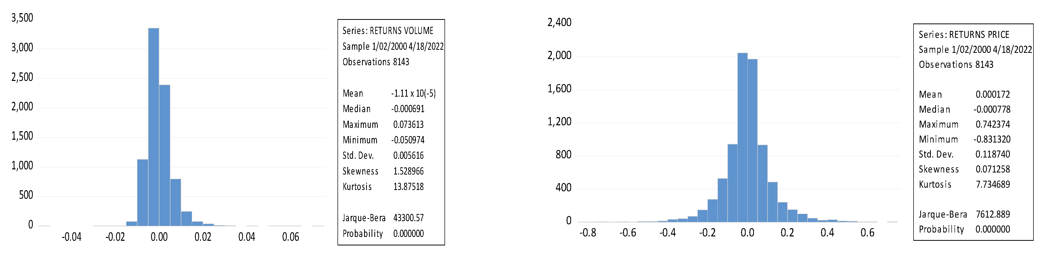
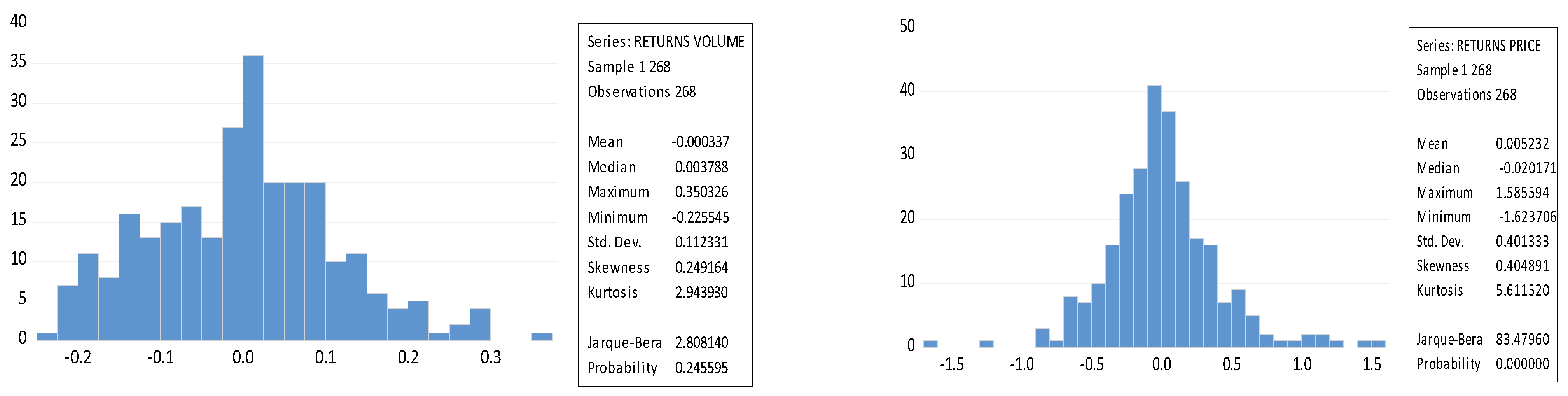
2. Data
3. Model
4. Results
5. Conclusions
Author Contributions
Funding
Data Availability Statement
Conflicts of Interest
References
- Cuaresma, J.C.; Hlouskova, J.; Kossmeier, S.; Obersteiner, M. Forecasting electricity spot-prices using linear univariate time-series models. Appl. Energy 2004, 77, 87–106. [Google Scholar] [CrossRef]
- Robinson, T.A. Electricity pool prices: A case study in nonlinear time-series modelling. Appl. Econ. 2000, 32, 527–532. [Google Scholar] [CrossRef]
- Escribano, A.; Peña, J.I.; Villaplana, P. Modelling Electricity Prices: International Evidence*. Oxf. Bull. Econ. Stat. 2011, 73, 622–650. [Google Scholar] [CrossRef]
- Knittel, C.R.; Roberts, M.R. An empirical examination of restructured electricity prices. Energy Econ. 2005, 27, 791–817. [Google Scholar] [CrossRef]
- Gianfreda, A.; Grossi, L. Zonal price analysis of the Italian wholesale electricity market. In Proceedings of the 2009 6th International Conference on the European Energy Market, Leuven, Belgium, 27–29 May 2009; pp. 1–6. [Google Scholar]
- Gianfreda, A. Volatility and volume effects in European electricity spot markets. Econ. Notes 2010, 39, 47–63. [Google Scholar] [CrossRef]
- Kraus, A.; Litzenberger, R.H. Skewness preference and the valuation of risk assets. J. Financ. 1976, 31, 1085–1100. [Google Scholar]
- Friend, I.; Westerfield, R. Co-skewness and capital asset pricing. J. Financ. 1980, 35, 897–913. [Google Scholar] [CrossRef]
- Fang, H.; Lai, T. Co-kurtosis and capital asset pricing. Financ. Rev. 1997, 32, 293–307. [Google Scholar] [CrossRef]
- Bessembinder, H.; Lemmon, M.L. Equilibrium pricing and optimal hedging in electricity forward markets. J. Financ. 2002, 57, 1347–1382. [Google Scholar] [CrossRef]
- Coelho Junior, L.M.; Fonseca, A.J.D.S.; Castro, R.; Mello, J.C.D.O.; Santos, V.H.R.D.; Pinheiro, R.B.; Sous, W.L.; Júnior, E.P.S.; Ramos, D.S. Empirical Evidence of the Cost of Capital under Risk Conditions for Thermoelectric Power Plants in Brazil. Energies 2022, 15, 4313. [Google Scholar] [CrossRef]
- Mayer, K.; Trück, S. Electricity markets around the world. J. Commod. Mark. 2018, 9, 77–100. [Google Scholar] [CrossRef]
- Ioannidis, F.; Kosmidou, K.; Savva, C.; Theodossiou, P. Electricity pricing using a periodic GARCH model with conditional skewness and kurtosis components. Energy Econ. 2021, 95, 105110. [Google Scholar] [CrossRef]
- Gillich, A.; Hufendiek, K. Asset Profitability in the Electricity Sector: An Iterative Approach in a Linear Optimization Model. Energies 2022, 15, 4387. [Google Scholar] [CrossRef]
- Qussous, R.; Harder, N.; Weidlich, A. Understanding power market dynamics by reflecting market interrelations and flexibility-oriented bidding strategies. Energies 2022, 15, 494. [Google Scholar] [CrossRef]
- Vega-Márquez, B.; Rubio-Escudero, C.; Nepomuceno-Chamorro, I.A.; Arcos-Vargas, Á. Use of Deep Learning Architectures for Day-Ahead Electricity Price Forecasting over Different Time Periods in the Spanish Electricity Market. Appl. Sci. 2021, 11, 6097. [Google Scholar] [CrossRef]
- Wang, J.; Wu, J.; Shi, Y. A Novel Energy Management Optimization Method for Commercial Users Based on Hybrid Simulation of Electricity Market Bidding. Energies 2022, 15, 4207. [Google Scholar] [CrossRef]
- Fanone, E.; Gamba, A.; Prokopczuk, M. The case of negative day-ahead electricity prices. Energy Econ. 2013, 35, 22–34. [Google Scholar] [CrossRef]
- Kyle, A.S. Continuous auctions and insider trading. Econom. J. Econom. Soc. 1985, 53, 1315–1335. [Google Scholar] [CrossRef]
- Chordia, T.; Huh, S.-W.; Subrahmanyam, A. Theory-based illiquidity and asset pricing. Rev. Financ. Stud. 2009, 22, 3629–3668. [Google Scholar] [CrossRef]
- Amihud, Y. Illiquidity and stock returns: Cross-section and time-series effects. J. Financ. Mark. 2002, 5, 31–56. [Google Scholar] [CrossRef]
- Vendrame, V.; Tucker, J.; Guermat, C. Some extensions of the CAPM for individual assets. Int. Rev. Financ. Anal. 2016, 44, 78–85. [Google Scholar] [CrossRef]
- Fabozzi, F.J.; Gupta, F.; Markowitz, H.M. The legacy of modern portfolio theory. J. Invest. 2002, 11, 7–22. [Google Scholar] [CrossRef]
- Jagannathan, R.; Skoulakis, G.; Wang, Z. Generalized methods of moments: Appl. Finance. J. Bus. Econ. Stat. 2002, 20, 470–481. [Google Scholar] [CrossRef]

| Panel A-OLS Regression-Augmented Volume Models | ||||
|---|---|---|---|---|
| Volume Model | Volume with Cokurtosis | Volume with Coskewness | Volume with Coskewness and Cokurtosis | |
| αt | 0.0001 | 0.0002 | 0.0008 | 0.0015 * |
| (0.1648) | (0.1880) | (0.8936) | (1.7959) | |
| λv,t−1 | −2.4937 *** | −2.7753 *** | −2.3919 *** | −0.9888 |
| −(10.8580) | −(14.0247) | −(5.5231) | −(1.4454) | |
| λcok,t | 23,769.2500 *** | −108,425.1000 *** | ||
| (3.3498) | −(3.2712) | |||
| λcos,t | 2984.7110 *** | 6469.6310 *** | ||
| (4.2303) | −(1.4454) | |||
| Number of Observations | 8143 | 8143 | 8143 | 8143 |
| R2 | 1.39% | 2.37% | 11.24% | 18.26% |
| Panel B-GMM Regression-Augmented Volume Models | ||||
| Volume Model | Volume with Cokurtosis | Volume with Coskewness | Volume with Coskewness and Cokurtosis | |
| αt | 0.1910 | 0.3204 | 0.1128 | 0.1014 * |
| (0.4532) | (0.1863) | (1.6223) | (1.7489) | |
| λv,t−1 | −2.3870 ** | −4.0577 * | −1.6265 * | −2.2640 ** |
| −(1.9906) | −(1.8855) | −(1.8456) | −(2.1043) | |
| λcok,t | 116,200.0000 | 155,753.6000 | ||
| (1.1829) | (1.1829) | |||
| λcos,t | 2368.5840 ** | 1408.9870 | ||
| (2.4344) | (0.7511) | |||
| J-statistic | 286.0240 | 127.9153 | 0.0034 | 0.3821 |
| Prob(J-statistic) | 0.0000 | 0.0000 | 0.9533 | 0.8261 |
| Number of observations | 7983 | 8105 | 8140 | 8141 |
| Panel A-OLS Regression-Augmented Volume Models | ||||
|---|---|---|---|---|
| Volume Model | Volume with Cokurtosis | Volume with Coskewness | Volume with Coskewness and Cokurtosis | |
| αt | 0.0049 | 0.0116 | 0.0250 | 0.0238 |
| (0.2903) | (0.6038) | (1.5969) | −(4.5916) | |
| λv,t | −1.1228 *** | −1.0365 *** | −0.3161 ** | −1.7855 *** |
| −(7.2201) | −(6.4252) | −(2.3306) | −(4.5916) | |
| λcok,t | 14.1173 | −59.4133 ** | ||
| (0.9771) | −(2.1511) | |||
| λcos,t | 21.2504 *** | 24.1067 ** | ||
| (4.0302) | (2.1066) | |||
| Number of Observations | 268 | 268 | 268 | 268 |
| R2 | 9.88% | 10.54% | 29.88% | 11.39% |
| Panel B-GMM Regression-Augmented Volume Models | ||||
| Volume Model | Volume with Cokurtosis | Volume with Coskewness | Volume with Coskewness and Cokurtosis | |
| αt | 0.0002 | 0.0454 *** | 0.0717 ** | −0.0090 |
| (0.0154) | (3.2133) | (2.1178) | −(0.2326) | |
| λv,t | −0.6205 *** | −0.4345 ** | 1.8413 * | 1.7868 * |
| −(4.4899) | −(2.4081) | (1.6634) | (1.6634) | |
| λcok,t | 86.7519 *** | −266.7234 ** | ||
| (4.0549) | −(2.1524) | |||
| λcos,t | 93.2383 *** | 127.6382 *** | ||
| (2.6517) | (0.0000) | |||
| J-statistic | 23.5120 | 27.4642 | 0.7926 | 1.9356 |
| Prob(J-statistic) | 0.1333 | 0.1560 | 0.3733 | 0.7476 |
| Number of observations | 250 | 247 | 266 | 265 |
Publisher’s Note: MDPI stays neutral with regard to jurisdictional claims in published maps and institutional affiliations. |
© 2022 by the authors. Licensee MDPI, Basel, Switzerland. This article is an open access article distributed under the terms and conditions of the Creative Commons Attribution (CC BY) license (https://creativecommons.org/licenses/by/4.0/).
Share and Cite
Cayon, E.; Sarmiento, J. The Impact of Coskewness and Cokurtosis as Augmentation Factors in Modeling Colombian Electricity Price Returns. Energies 2022, 15, 6930. https://doi.org/10.3390/en15196930
Cayon E, Sarmiento J. The Impact of Coskewness and Cokurtosis as Augmentation Factors in Modeling Colombian Electricity Price Returns. Energies. 2022; 15(19):6930. https://doi.org/10.3390/en15196930
Chicago/Turabian StyleCayon, Edgardo, and Julio Sarmiento. 2022. "The Impact of Coskewness and Cokurtosis as Augmentation Factors in Modeling Colombian Electricity Price Returns" Energies 15, no. 19: 6930. https://doi.org/10.3390/en15196930
APA StyleCayon, E., & Sarmiento, J. (2022). The Impact of Coskewness and Cokurtosis as Augmentation Factors in Modeling Colombian Electricity Price Returns. Energies, 15(19), 6930. https://doi.org/10.3390/en15196930