Short-Term Load Forecasting Using EMD with Feature Selection and TCN-Based Deep Learning Model

Abstract

Short-term load forecasting (STLF) has a significant role in reliable operation and efficient scheduling of power systems. However, it is still a major challenge to accurately predict power load due to social and natural factors, such as temperature, humidity, holidays and weekends, etc. Therefore, it is very important for the efficient feature selection and extraction of input data to improve the accuracy of STLF. In this paper, a novel hybrid model based on empirical mode decomposition (EMD), a one-dimensional convolutional neural network (1D-CNN), a temporal convolutional network (TCN), a self-attention mechanism (SAM), and a long short-term memory network (LSTM) is proposed to fully decompose the input data and mine the in-depth features to improve the accuracy of load forecasting. Firstly, the original load sequence was decomposed into a number of sub-series by the EMD, and the Pearson correlation coefficient method (PCC) was applied for analyzing the correlation between the sub-series with the original load data. Secondly, to achieve the relationships between load series and external factors during an hour scale and the correlations among these data points, a strategy based on the 1D-CNN and TCN is proposed to comprehensively refine the feature extraction. The SAM was introduced to further enhance the key feature information. Finally, the feature matrix was fed into the long short-term memory (LSTM) for STLF. According to experimental results employing the North American New England Control Area (ISO-NE-CA) dataset, the proposed model is more accurate than 1D-CNN, LSTM, TCN, 1D-CNN–LSTM, and TCN–LSTM models. The proposed model outperforms the 1D-CNN, LSTM, TCN, 1D-CNN–LSTM, and TCN–LSTM by 21.88%, 51.62%, 36.44%, 42.75%, 16.67% and 40.48%, respectively, in terms of the mean absolute percentage error.

1. Introduction

As a basic industry supporting national construction, the power industry plays an increasingly important role in our daily life [1]. In recent years, to cope with the adverse effects of climate change, non-fossil energy sources such as solar, wind, and geothermal energy have been rapidly developed in the power industry. Short-term power load forecasting (STLF) plays an important role in the control of smart grids, power security, power supply planning, and rational dispatch planning [2]. The rationality of power supply planning is related to the effective use of fossil and non-fossil energy sources, and directly affects the achievement of climate change goals in China. In addition, it has been demonstrated that operating costs will increase by 10 million pounds due to a 1% increase in forecasting error [3]. Therefore, the improvement of accuracy of STLF is of great significance to the safe and economic operation of the power systems. However, electricity consumption is usually stochastic. Furthermore, external factors such as temperature and day type can also affect the changes in energy use, resulting in a highly nonlinear and non-stationary load series, which poses a great challenge for load forecasting.

Many researchers have studied STLF over the past few decades. In the early years, these predictive studies were largely based on traditional methods with mathematical statistics, such as regression analysis [4], the auto-regressive integrated moving average (ARIMA) method [5], and the Kalman filter [6]. Although traditional methods are useful in forecasting linear time series [7], they cannot be adopted to predict the nonlinear and non-stationary load sequences. To effectively tackle nonlinear features fitting in load series, several intelligent algorithms based on machine learning methods have been used for load prediction, such as support vector regression (SVR), artificial neural networks (ANN), random forest methods (RF), and extreme learning machines (ELM). Jiang et al. [8] proposed a hybrid forecasting model based on the SVR and hybrid parameter optimization algorithms. Their experiments demonstrate that the SVR model tuned by the two-step hybrid optimization algorithm achieves better performance than some traditional models in STLF. However, the SVR model has shortcomings, such as a highly complex optimization process and slow convergence. Guo et al. [9] proposed a novel STLF model that combined several machine learning methods, such as SVR, grey catastrophe (GC (1,1)), and random forest (RF) modeling, which addressed the shortcomings of SVR by the hybrid model and fast convergence performance of RF. Wei et al. [10] compared seven machine learning and deep learning algorithms; SVR, extreme gradient boosting (XGBoost), and long short-term memory (LSTM) were judged as the most accurate models. Their results indicated that machine learning methods can model complex and nonlinear relationships between power load and external factors to improve the accuracy of load forecasting [11]. However, due to the increasing scale of input data, the machine learning models easily fall into the local optimum and rely on manual parameter adjustment. Deep learning provides a promising solution for effectively handling massive data. Therefore, in recent years, deep learning models have been widely used in time series.

The LSTM, a representative sequence prediction model, is a variant of a recurrent neural network (RNN) and can deal with long-term dependencies implied in time series. Jiao et al. [12] proposed a method to predict the load of non-residential consumers using multiple correlated sequence information based on the LSTM, which considered the effects of multiple related sequences, such as adjacent time points, the same time points of adjacent days, and the same day in adjacent weeks among data samples for a specific consumer. Kong et al. [13] proposed a LSTM–RNN based load forecasting framework for residential load forecasting, which employed density based clustering technique to reflect the lifestyles of different residents into energy consumption. These aforementioned methods demonstrate that the LSTM can successfully capture the temporal dependencies of time series. In [14], LSTM, gated recurrent network, and convolutional neural network (CNN) were trained and compared to the forecast 1 day to 7 days ahead of the daily electricity load. The forecasting results on the test set showed that the best performance was achieved by LSTM. Considering the temporal dependencies implied in the load series, the LSTM was selected as the predictor of the proposed model in this study. However, external factors such as temperature and day types can also affect the changes in energy use, resulting in a highly nonlinear and non-stationary load series. Therefore, it struggles to make accurate predictions by using single load series as input.

Some researchers believe that it is necessary to use a pre-processing method such as decomposition of original sequences to reduce the complexity of load series. The decomposition methods of original load series usually consists of wavelet transform (WT) and empirical mode decomposition (EMD). The WT has the advantage of localization, but rationalizing the wavelet basis and decomposition scale is a difficult task. When compared with wavelet decomposition, the EMD method is intuitive, direct, and adaptive. It does not require any predefined basis function and overcomes the difficulty of choosing wavelet basis function in wavelet transform. Zheng et al. [2] proposed a hybrid algorithm that combines a similar day selection, EMD, and LSTM. The hidden information in the load series was mined by the EMD and used as input to the LSTM along with external factors such as temperature and day types. Hong et al. [15] applied the EMD to decompose the load series into several intrinsic mode functions (IMFs)and a residual term, which were further defined as three items and modeled separately by the SVR-based model. These two models demonstrated that the EMD decomposition technique can effectively transform the nonlinear load series into a number of simple and stable sub-series, which improves the performance of the prediction model. Most researchers have built prediction models for each sub-series, but this will increase the complexity of the models significantly. In this paper, the sub-series with high correlations with the original load data were selected by the Pearson’s correlation coefficient (PCC) method as the input features, and the constructed serial structure greatly reduces the overall complexity of the prediction model when compared with the model established for each sub-series. Meanwhile, the increase of diversity of input data has placed higher requirements for the feature extraction capability of the prediction model. Due to the lack of convolution in the LSTM network, the feature extraction capability of the prediction model should be enhanced through being combined with other deep neural networks.

It is well known that integrating different single models to extract different patterns of features can overcome some drawbacks of the original model, which can improve the accuracy of prediction. The most widely used technique in deep learning is the CNN, which has made great progress in the field of image recognition [16]. The CNN can capture the nonlinear trend of the input data and consider correlations between multiple variables. Because of the high flexibility of the CNN structure [17], it is often combined with other models for feature extraction in the prediction of time series. Sadaei et al. [18] proposed a combined method that is based on the fuzzy time series (FTS) and CNN; multivariate time series data was converted into multi-channel images to be fed to a proposed deep learning CNN model with proper architecture. However, the CNN has difficulty in capturing the temporal features of long-time series. Imani et al. [19] proposed a hybrid algorithm that combined CNN and SVR for load forecasting. Kim et al. [20] proposed a network that combined CNN and LSTM to extract spatial and temporal features to predict housing energy consumption. These two models mentioned above achieved good forecasting results, and overcame the disadvantage that the CNN cannot capture the temporal dependences of long-time series. However, the large number of parameters in the CNN algorithm can cause overfitting of the prediction model and then reduce the forecasting accuracy. Compared with CNN, one-dimensional CNN (1D-CNN) has fewer learnable parameters, which can address the overfitting problem. In addition, Bai et al. [21] pointed out that temporal convolutional network (TCN) can effectively expand the receptive field through its unique dilated convolutional structure, so that the output can receive a larger range of input information, which makes it more advantageous than most sequence models in extracting temporal features. Since then, the TCN-based models were deeply studied in STLF [22,23], and have a better predictive performance. In order to compensate for the shortcomings of CNN and achieve comprehensive feature extraction of input data, we propose a feature extraction method based on 1D-CNN and TCN.

Many researchers have used attention mechanisms (AM) in combination with other models to fully exploit the important relationships between load data and external factors. It means that the AM can select key information from the features of the input and be used to solve the issue that models such as LSTM cannot recognize the important features. Tang et al. [24] proposed a short-term load forecasting model based on TCN with channel and temporal attention mechanism (AM), which performed well in the experimental dataset. Ding et al. [25] proposed a data-driven intelligent flood forecasting model based on spatio-temporal attention and LSTM. The experimental results showed that the attention-based models can achieve better accuracy than the benchmarks. The self-attention mechanism (SAM), a variant of AM, is better at capturing the internal correlation of input features. Ju et al. [26] established an encoder–decoder model based on the SAM, which used the SAM to capture the long-distance sequence information and achieved good results. Motivated by this, in order to provide effective input features to the LSTM, a feature extraction and enhancement module based on 1D-CNN–TCN–SAM was developed and validated in this study.

On the basis of the foregoing research, this paper presents an integrated model with feature selection that combines EMD, PCC, 1D-CNN, TCN, SAM, and LSTM to predict short-term load. Firstly, the EMD-based feature selection (EFS) module consists of the algorithms of EMD and PCC. The original load series were decomposed by the EMD and then the PCC [27] was applied for feature selection. The hidden information in the original load series can be mined due to being linearized and smoothed, which provides effective input features for the training model. Secondly, the feature extraction and enhancement module consists of the algorithms of 1D-CNN, TCN, and SAM. The serial structure of 1D-CNN and TCN was used for feature extraction. The 1D-CNN extracts the correlations of load-related influencing factors, and the TCN can capture the temporal dependences of load series. However, this process does not learn the dependencies of distant positions and cannot select key information from the feature matrix. In terms of this, the SAM was used to capture the internal correlation information of all time steps and obtain the feature weight of each time step. Then, we obtained a key feature matrix with both the correlations between load series and external factors and the temporal dependences between adjacent time points. The key feature matrix was fed into the LSTM to obtain the final prediction. When compared with other existing models, experimental results show that the proposed model has superior performance and robustness. The main contributions of this paper can be summarized as follows:

• The EFS module can select the sub-series decomposed by EMD with high correlation with the original load data as the input features of the training model, which not only promotes the mining the hidden information in the load data, but also reduces the redundant information.
• The feature extraction and enhancement module is able to extract effective features from the input data, including correlations between multiple variables and temporal dependencies between different time steps. Meanwhile, the SAM focuses on the key information of the feature matrix to provide effective input for the LSTM.
• Experimental results demonstrated that the feature matrix with dynamic weights makes a significant improvement in the prediction performance of LSTM.
• The experimental results were evaluated using multiple feature extraction methods at the same time scale, and were compared with other state-of-the-art models. The comparison results demonstrated that the proposed model has superior performance and stability in STLF.

The remainder of this paper is organized as follows. Section 2 presents the model algorithms of the prediction method in this paper. Section 3 describes the experimental design and analysis of this study. Finally, Section 4 briefly presents the study conclusions and outlook.

2. Methodology

This section introduces the basic theories of EMD, PCC, 1D-CNN, TCN, SAM, and LSTM, respectively, and shows the framework of the proposed model in detail. In addition, the content of this section will be presented according to the following three main processes: feature selection, feature extraction and enhancement, and load prediction.

2.1. Feature Selection

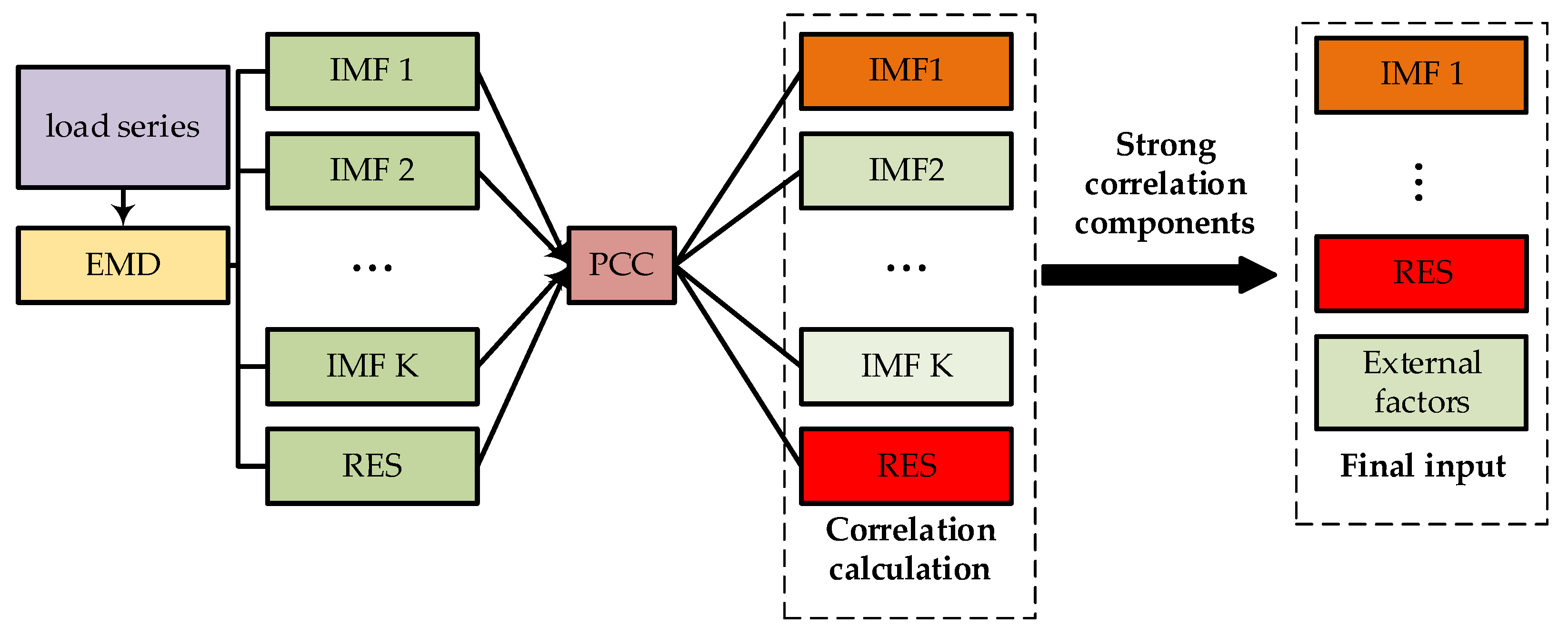
The EFS module consists of the algorithms of EMD and PCC. Because the EMD is adaptive in series decomposition and can theoretically decompose any kind of signal, it favors processing any nonlinear and non-smooth time series. The original load series can be decomposed into a set of IMFs and a residue term. If all of these decomposed sub-series and the residue term are used as the input features for feature extraction, it will not only increase the computational cost, but also tend to overfit due to a large number of model parameters [28]. Therefore, we used the PCC to analyze the correlation between the IMF components and the original load series, and selected the components with strong correlations with the original load series as the input features, which is beneficial to providing effective features for the prediction model [29]. The flow-chart of the EFS module is shown in Figure 1 and the principles of the EMD and PCC are described in detail below.

2.1.1. Empirical Mode Decomposition

The EMD is a signal processing method inventively proposed by Huang et al. [30], which is widely used in the area of signal processing. The EMD can decompose a complicated signal into a set of IMFs and a residue term [31], and each IMF component should satisfy the following two conditions:

• For each IMF sequence, the difference between the number of extreme points and zero-crossing points must be equal to one;
• At any point, the average value of the envelope defined by the local maximum and local minimum must be zero.

By analyzing each IMF component that involves the local features of a signal, the information of the features of the original load series could be extracted more accurately and effectively. The specific steps of the EMD algorithm are summarized as follows:

• A signal $x\left(t\right)$ is firstly identified for its all maxima and minima. Then, the average envelope curve $m_1\left(t\right)$ can be obtainedby calculating the mean of the upper envelope $u\left(t\right)$ and lower envelope $l\left(t\right)$, i.e.,

$$m_1\left(t\right)=\frac{u\left(t\right)+l\left(t\right)}{2} \left(1\right)$$

(1)

2.

The difference between the signal $x\left(t\right)$ and $m_1\left(t\right)$ is the first IMF candidate $h_1\left(t\right)$:

$$h_1\left(t\right)=x\left(t\right)-m_1\left(t\right)$$

(2)

If $h_1\left(t\right)$ satisfies the two conditions of the IMF, then it is the first IMF of $x\left(t\right)$. Thus, it can be considered as $im{f}_1\left(t\right)$.

3.

If $h_1\left(t\right)$ cannot satisfy the two conditions of the IMF, it should be regarded as the original signal, and the above steps will be repeated until the two conditions are satisfied. Assuming that the process is repeated $n$ times and then $h_{1n}\left(t\right)$ can be shown as:

$$h_{1n}\left(t\right)=h_{1\left(n-1\right)}\left(t\right)-m_{1n}\left(t\right)$$

(3)

where $h_{1n}\left(t\right)$ ($h_{1\left(n-1\right)}\left(t\right)$) presents the signal after shifting $n$($n$−1) times. $m_{1n}\left(t\right)$ is the average envelope of $h_{1n}\left(t\right)$. Then, $h_{1n}\left(t\right)$ is designated as $im{f}_1\left(t\right)$.

4.

A new signal $r_1\left(t\right)$ can be generated by subtracting the $im{f}_1\left(t\right)$ from the $x\left(t\right)$:

$$r_1\left(t\right)=x\left(t\right)-im{f}_1\left(t\right)$$

(4)

5.

$r_1\left(t\right)$ is treated as the original signal to obtain $im{f}_2\left(t\right)$. Steps 1 to 4 will be repeated $k$ times until a residual term $r_k\left(t\right)$ is a monotonic function, i.e.,

$$x\left(t\right)={\displaystyle \sum }_{i=1}^{k}im{f}_i\left(t\right)+r_k\left(t\right)$$

(5)

With the aforementioned steps, we can eventually obtain $k$ IMFs $(im{f}_1\left(t\right), im{f}_2\left(t\right),\dots ,im{f}_k\left(t\right))$ and a residue term $r_k\left(t\right)$.

2.1.2. Pearson’s Correlation Coefficient

An original load series can be decomposed into a number of sub-series and a residue term by using the EMD. If we establish some prediction models for each sub-series, it will lead to a large prediction error due to multiple random errors and some noise interferences. Therefore, feature selection is important for reducing the complexity of the prediction models. In this paper, the PCC was used to feature selection. In general, the correlation coefficient $\rho (·)$ between two vectors $X$ and $Y$ can be defined as:

$${\rho }_{X,Y}=\frac{\mathrm{COV}\left(X,Y\right)}{{\sigma }_X{\sigma }_Y}=\frac{\mathrm{E}\left(XY\right)-\mathrm{E}\left(X\right)\mathrm{E}\left(Y\right)}{\sqrt{\mathrm{E}\left(X^2\right)-{\mathrm{E}}^2\left(X\right)}\sqrt{\mathrm{E}\left(Y^2\right)-{\mathrm{E}}^2\left(Y\right)}}$$

(6)

where $X$ and $Y$ are the two random variables, $\mathrm{COV}(·)$ is the covariance, and $\mathrm{E}(·)$ represents the mathematical expectation. The PCC uses the valueof Equation (6) as an indicator to evaluate individual features. We can choose the decomposed sub-series with large correlations with the original load series as the input features of the prediction model according to the above criteria.

2.2. Feature Extraction and Enhancement

In this section, a simple and effective structure of feature extraction is constructed based on the 1D-CNN and TCN. Firstly, the 1D-CNN with three different convolutional kernels (2, 3, and 4) was used to extract local information between different input features. The local features of different dimensions were processed into the same dimension by the pooling process, and the resulting feature maps were fused together as the input of the TCN. Secondly, the TCN was used to capture temporal dependencies of time series. Furthermore, the SAM was introduced to dynamically adjust the weight of the information of different features to enhance the key features. The flow-chart of the feature extraction and enhancement module is shown in Figure 2.

2.2.1. One-Dimensional Convolutional Neural Network

The CNN is a type of deep neural network with convolutional, activation, and pooling layers, and has superior performance in many nonlinear data. In this paper, 1D-CNN is applied to extract correlation between different input features. The principle of 1D-CNN is shown in Figure 3 and then the convolution process is described as follows:

• At the convolutional layer, the convolution filter with a fixed length slides over the input of load data to form feature maps. The size of the feature map can be controlled by adjusting the size of the convolution kernel and the step size. Thus, the structure of CNN is highly flexible.
• The activation layer is a non-linear operation of the CNN model that learns the non-linear representation of the feature maps by a non-linear activation function such as the logistic function (sigmoid), the tangent function (tanh), or the rectified linear activation function (ReLU). The mathematical model of the convolutional layerand activation layer is described as:

$$H=f\left(I*W+b\right)$$

(7)

where $H$ and $I$ indicate the output matrix and input matrix, respectively. $W$ and $b$ indicate the weight matrix and the corresponding bias vector of the convolution kernel, respectively. $*$ indicates for convolution operation, and $f(·)$ indicates the activation operations.

3.

The pooling layer can obtain the final feature map by some nonlinear numerical calculations, e.g., the average pooling or maximum pooling. This process can reduce the spatial dimensions of the feature map and the number of parameters of the network.

Thus, local features can be extracted between the input on a time pointby adjusting the parameters of the convolutional and pooling layers.

2.2.2. Temporal Convolutional Network

The TCN is an innovation and improvement of the 1D-CNN. It can capture long-range patterns by using a hierarchy of causal convolution, dilated convolution, and residual block, unlike the 1D-CNN. Moreover, the TCN has the following advantages:

• The disclosure of future information problem is prevented by the causal convolution.
• The receptive field of the structure is expanded by using the dilated convolution.
• The historical information can be maintained for a long time by using the residual block.

Each module of the TCN will be described in the following section.

Causal convolution is a one-way model with strict time constraints. As shown in Figure 4a, the output $y_t$ in the time step $t$ only depends onthe input of the layers ($x_{t-4}, x_{t-3}, x_{t-2}, x_{t-1}, x_t$) at that moment and before. That is to say, the output sequence of the network is only influenced by the information from the past input, avoiding the disclosure of future information. Therefore, the structure of causal convolution is more in line with the inherent law of load. However, the causal convolution is easily limited by the receptive field.

In order to capture the long-time dependence of time series, the receptive field of the convolutional structure should be large enough. As shown in Figure 4b, when using the causal convolution, the receptive field can be expanded by increasing the number of network layers, as well as the filter size and the time steps. However, these methods can result in the vanishing of gradients, overfitting, and the leakage of valid information. To overcome these problems, the TCN introduces a dilated convolution on top of the causal convolution [32]. For a time series input $X=\left[x_0,\cdots ,x_N\right]$ and a filter $f$ whose filter size is $k$, the dilated convolution operation $F(·)$ of the sequence element $N$ is defined as:

$$F\left(N\right)=\left(X{*}_{d}f\right)\left(N\right)={\displaystyle \sum }_{i=0}^{k-1}f\left(i\right)*X_{N-d·i}$$

(8)

where $d$ and $k$ are the dilation factor and convolution kernel size, respectively, and $N-d·i$ explains the orientation of the convolution. By increasing the dilation factor $d$, the TCN effectively increases the receptive field without the increase of the computational cost. It is clear that Figure 4b shows the structural advantages of the dilated convolution.

With the deepening of the network, the parameters of the network model increase, and then this will lead to a series of problems such as the vanishing of gradients and the decrease of the accuracy of the training set. To conquer these problems, the residual connections were introduced to the TCN. The details of the residual modules are shown in Figure 5a. One can find that there are two layers of dilated causal convolution in each residual block and the convolution filter is weighted with normalization. Besides, a dropout layer was added to the dilated convolution for regularization. In this paper, we chose the self-gated activation function (SiLU) as the activation function. The SiLU function is a combination of the sigmoid function and the ReLU function that is more effective than the ReLU function in most cases due to its smooth feature [33]. The residual block uses a 1 × 1 convolution to ensure the same dimensions of the input and output. Figure 5b shows the deep TCN formed by stacking multiple residual modules. The constructed deep TCN enables the network to look back deeply into the historical series to establish long-time dependencies.

2.2.3. Self-Attention Mechanism

The attention mechanism simulates the mechanism of human visual attention that selects the more critical information from numerous input features by weight assignment [25]. The principle of SAM is shown in the Figure 6, which linearly maps the input sequence $X$ into three different matrices $\left(Q,K,V\right)$ by three different weight matrices $(W_q,W_k, W_v)$. Then, we can use the scaled dot product as the attention scoring function to obtain the attention weight matrix $W$. Finally, the output matrix is obtained by multiplying $W$ with $V$. This process focuseson the correlation of internal features of the input matrix and establishes the dependencies of the global features to enhance the key features of the input series and reduce the influence of external information. The SAM is defined as follows:

$$\{\begin{array}{c}Q=W_{q}X\\ K=W_{k}X\\ V=W_{v}X\end{array}$$

(9)

$$W=softmax\left(\frac{K^{T}Q}{\sqrt{D_k}}\right)$$

(10)

$$Attention=WV=softmax\left(\frac{K^{T}Q}{\sqrt{D_k}}\right)V$$

(11)

where $W_q, W_k,$ and $W_v$ are the linear mapping weight matrices. $Q, K,$ and $V$ representthe query, key, and value, respectively. $softmax(·)$ is the normalization function by the column, $D_k$ is the dimension of $K$, and $\frac{1}{\sqrt{D_k}}$ is the scaling factor.

2.3. Load Prediction

LSTM is a variant of the RNN that overcomes the vanishing or explosion of gradients of the latter when processing the long-term dependencies of load series. Through adding the input, output, and forget gates to the RNN, the LSTM can effectively handle the long-term dependencies of time series, and has been widely used in natural language processing [34], machine translation [35], load forecasting [36], and other fields. The LSTM was used as a predictor of STLF in this study. The global features that dynamically weigh the key features of input data and external factors were used as the input for the LSTM to improve the accuracy of load forecasting.

Figure 7 shows the architecture of the LSTM memory block. The LSTM network introduces a gating mechanism to control the transfer path of the information, and each neuron consists of three gate structures: the forget gate $f_t$, input gate $i_t$, and output gate $o_t$. Specifically, the forget gate $f_t$ controls how much information needs to be forgotten from the cell state $c_{t-1}$. The input gate $i_t$ updates the memory cell state using the information from the current input and previous hidden state. The output gate $o_t$ controls the selective output of the current memory cell state.

The formulas of all the cells of LSTM are represented in following equations.

$$f_t=\sigma \left(W_f{x}_t+R_f{h}_{t-1}+b_f\right)$$

(12)

$$i_t=\sigma \left(W_i{x}_t+R_i{h}_{t-1}+b_i\right)$$

(13)

$${\tilde{c}}_t=tanh\left(W_c{x}_t+R_c{h}_{t-1}+b_c\right)$$

(14)

$$o_t=\sigma \left(W_o{x}_t+R_o{h}_{t-1}+b_o\right)$$

(15)

$$h_t=o_t\cdot tanh\left(c_t\right)$$

(16)

$$c_t=f_t{c}_{t-1}+i_t{\tilde{c}}_t$$

(17)

where $W_f, W_i, W_c, W_o, R_f, R_i, R_c$ and $R_o$ represent the corresponding weight matrices to be learned. The vectors $b_f, b_i, b_c$ and $b_o$ are the corresponding bias matrices. $c_t$ and ${\tilde{c}}_t$ denote the current values and new candidate values for cell state, respectively. There are two activation functions, i.e.,$\sigma (·)$(sigmoid) and $tanh(·)$, forthe update of cell state and the selective output.$x_t$ and $h_t$ are the input and output at time step t, respectively. The memory unit can retain the key information at an early moment for a certain time interval by using the gating mechanism, so it can capture the long-range dependencies and solve the problem of gradient vanishing of the RNN.

2.4. Framework of the Proposed Model

In this paper, a novel integrated model using the EFS module and TCN-based deep learning model was designed to effectively forecast short-term power load. Figure 8 shows the flow-chart of short-term load forecasting and the data conversion process of the proposed model. The input data is a matrix of 24 × 13, which includes the strongly correlated IMF components provided by the EFS module, original load series, and external features. The flow-chart of the proposed model is described as follows.

Step 1: The input matrix was first extracted by three one-dimensional convolutions with kernels of 2, 3, and 4, respectively, to obtain the local correlations of different influencing factors at different time scales. The convolution process yielded three one-dimensional matrices,$Y_1$, $Y_2$ and $Y_3$, respectively. Three one-dimensional matrices were processed into the same length by the pooling process and concatenated into a matrix $Y$ of 18$*$3.

Step 2: The TCN was used to establish the temporal dependencies of these features. The output generated in Step 1 was processed by the TCN to obtain a matrix of 12 $*$3 that contains the local correlations of the different influencing factors and the preliminarily established temporal dependencies. Then, the matrix was given dynamic weights by the SAM to highlight key features.

Step 3: The feature matrix obtained in Step 2 was input into the LSTM to establish the mapping relationships with labels to obtain the predicted value, and the error value $e_1$ was calculated using the predicted value and the actual value.

Step 4: Steps 1 to 3 were repeated for multiple epochs, each of which updated the weights of each connection of the model by gradient descent. If $e_1$ is less than the expected error $e_2$, the model would be saved and used to obtain the final prediction for the test set, otherwise, the model parameters need to be adjusted.

3. Experimental Results and Analysis

This section conducted a series of experiments on a public data set to evaluate the effectiveness of the proposed model. In addition, several TCN-based or EMD-based models were employed to compare with our model. All these models will be run in the Python 3.7 environment using Pytorch 1.7 as back ends, and the hardware of the PC was an AMD-5800H CPU @ 3.8 GHz and NVIDIA RTX 3060 GPU with 16GB of memory. In the following, we will introduce the experimental design, feature selection analysis, and prediction results.

3.1. Experimental Design

3.1.1. Dataset

The experimental design and analysis is based on an open dataset of New England, USA that consists of the power data, temperature, and date type from 1 March 2003 to 31 December 2014. The resolution of the dataset is one hour. Furthermore, we only selected a total of 40,392 data points from 1 March 2003 to 8 October 2007, in which a total of 22,872 data points were used as the training set, 8760 data points were used as the validation set, and 8760 data points were used as the test set.

3.1.2. Sliding Window Settings

The length of the sliding window is essentially the time step of the TCN, so that a suitable sliding window has a key role in the improvement of prediction accuracy. In this paper, the sliding window had a length of 24 h and a step size of one hour. The input feature matrix contains the load series and external feature factors for 24 h prior to the forecast point. The settings of the sliding window mentioned above are beneficial to the establishment of time-dependent relationships.

3.1.3. Comparative Models

In order to evaluate the superior performance of the proposed model, the comparative models are set up as follows:

• The models of CNN, LSTM, TCN, CNN–LSTM, and TCN–LSTM were used for comparison with the CNN–TCN model, for demonstrating the effectiveness of feature extraction with the CNN–TCN model.
• The EFS module was combined with each aforementioned model, for demonstrating the effectiveness of it.
• The SAM module was added to all these models for studying the improvement of accuracy for load forecasting.

In order to further verify the effectiveness and stability of the proposed model, we conducted the experimental analysis under different time ranges by adjusting the test set. Then, the data from January, April, July, and October in the original test set were selected as the sub-sets to validate the influence of different seasons on the performance of the proposed model. Moreover, the data from a week were also selected as a sub-set to compare the performance of load forecasting on weekdays with that of weekends.

3.1.4. Evaluation Criteria

In this paper, the mean absolute percentage error (MAPE) and root mean square error (RMSE) were considered as evaluation indices to evaluate these models. The smaller the errors of the statistical metrics are, the higher the accuracy of the load forecasting is in general. The statistical metrics are defined as follows:

$$MAPE=\frac{1}{n}{\displaystyle \sum }_{i=1}^n\left|\frac{{\widehat{y}}_i-y_i}{y_i}\right|$$

(18)

$$RMSE=\sqrt{\frac{1}{n}{\displaystyle \sum }_{i=1}^n{({\widehat{y}}_i-y_i)}^2}$$

(19)

where $n$ is the number of predicted time points, ${\widehat{y}}_i$ and $y_i$ represent the predicted value and the true value at the $i$-th time point, respectively.

3.2. Feature Selection Analysis

3.2.1. Selection and Analysis of External Factors

To demonstrate the correlation between the temperature and load data, we collected the data of temperature and power load from 8 October 2005 to 8 October 2008. Figure 9 shows the evolution of the power load and temperature for three years. It is clear that the power consumption peaks when the temperature is very high or low. That is to say, there is a positive correlation between load and temperature in summer, whereas the correlation becomes negative in winter.

Figure 10 shows the profile of power load for 14 days. One can find that the load demand has a certain regularity, i.e., weekday load tends to be higher than that of the weekend load, especially on Monday and Tuesday. In addition, weekends, holidays, and special festivals have different electricity consumption patterns than weekdays, often causing fluctuations in electricity consumption. Therefore, this paper considered temperature, holidays, weekends, and seasons as the external features of the input matrix.

The attributes of features such as weekdays, holidays, and seasons were encoded using the one-hot encoder. To enhance the convergence speed of the model and strengthen the mapping relationship between the data, the power load and temperature were normalized by the Min–Max. The normalization principle is defined as:

$$\widehat{x}=\frac{x-\min \left(X\right)}{\max \left(X\right)-\min \left(X\right)}$$

(20)

where $X$ is the entire time series, $\max (·)$ is the maximum value of the entire series, $\min (·)$ is the minimum value of the entire series, $x$ is the data before normalization, and $\widehat{x}$ is the data after normalization.

3.2.2. Decomposition Results and Selection of EMD

The original load series was decomposed into multiple IMF components and a residual term by the EMD, and the decomposition results of load data are shown in Figure 11. The figure shows all components in the order from high to low frequencies, and each component contains different trends and local features at different time scales. It can be observed that the high-frequency component is mainly influenced by sudden events and the habits of daily fixed power consumption, while the low-frequency component shows that the influence of temperature and other external factors on load consumption is a slowly changing process. Furthermore, we obtained the statistical information of all IMF components as shown in

Table 1. Statistical information for each IMF component decomposed by using the EMD.

Data	Mean. (MW)	Max. (MW)	Min. (MW)	SD.	Skew.
Raw Data	14,896	27,622	8820	2931.05	0.29
IMF 1	−59.42	5067.13	−5131.46	664.54	0.106
IMF 2	134.06	7348.69	−6856.20	1400.46	0.007
IMF 3	3.29	4609.20	−4598.07	1594.63	0.01
IMF 4	−3.00	2944.46	−2890.86	412.39	0.04
IMF 5	9.35	3637.02	−4504.12	563.53	−0.03
IMF 6	17.00	2914.79	−2786.95	766.66	0.05
IMF 7	0.087	2450.95	−2415.05	509.15	−0.06
IMF 8	−17.26	1905.86	−1749.05	478.56	0.17
IMF 9	2.79	1760.84	−2386.01	837.01	−0.35
IMF 10	−161.81	1569.21	−1902.19	933.17	0.03
IMF 11	69.87	804.69	−623.47	421.08	0.005
IMF 12	2.13	185.03	−179.45	96.23	−0.08
Residual	14,898.72	15,042.27	14,746.51	112.62	−0.07

, including maximum (Max.), minimum (Min.), mean value (Mean.), standard deviation (SD.), and skewness (Skew.). The standard deviation is most often used in probability statistics as a measure of the degree of statistical distribution, reflecting the degree of dispersion between individuals within a series. The skewness describes the degree of asymmetry in a distribution. The closer the value of skewness is to zero, the closer the sample is to normal distribution [37]. It is clear that the standard deviation of each IMF component is significantly decreased when compared with that of the original load data, which indicates these decomposed sub-series show more smoothness and stability. According to the skewness values in Table 1, these IMFs decomposed by the EMD are closer to a normal distribution than the original data, which is beneficial for training the model.

Table 2. Correlation results of each IMF component by the PCC method.

component coefficient	IMF 1	IMF 2	IMF 3	IMF 4	IMF 5	IMF 6
	0.32	0.58	0.56	0.1	0.2	0.27
	IMF 7	IMF 8	IMF 9	IMF 10	IMF 11	IMF 12
	0.17	0.16	0.23	0.29	0.05	−0.0075

shows the correlation coefficients of each IMF component and the original load data. Among them, the IMF 2 and IMF 3 have a strong correlation with the raw load data, and the trend of IMF 10 reflects the changing characteristics of seasons and shows a relatively high correlation in low-frequency components. Finally, the residual term reflects the overall trend of load data. Therefore, the decomposed components of IMF 2, IMF 3, IMF 10, and the residual term were selected as the input features of the training model.

3.2.3. Input of the Model

After being filtered by the EFS module, the final features of the input can be defined as:

$$I=\left\{IM{F}_1,IM{F}_2,\dots ,IM{F}_{n-1},RES\right\}$$

(21)

$$Data\_input=\left\{I_o,I_s,I_h\right\}$$

(22)

where $I$ denotes the decomposed components of the original load data, and $IM{F}_i$ and $RES$ denotes the decomposed components and the residual term, respectively.$I_o$ denotes the external factors of the inputsuch as temperature, weekend, and season, etc. $I_s$ denotes the optimal sub-series by using the PCC, and $I_h$ denotes the original load data. $Data\_input$ denotes the final features of the input that include the external factors, the optimal sub-series, and the original load. The reconstructed dataset was fed into the algorithms for feature extraction.

3.3. Comparative Analysis of Different Forecasting Models

In order to verify the influence of the EFS, SAM, and 1D-CNN–TCN–LSTM modules on the performance of STLF, we established some comparative models, and compared them under three cases: the original model (Case A), the model with the EFS module (Case B), and the model with EFS and SAM modules (Case C).

Table 3. Comparison of experimental prediction results.

Model	Case A: Original Model		Case B: Combined with the EFS Module		Case C: Combined with the EFS and SAM Modules
	MAPE (%)	RMSE (MW)	MAPE (%)	RMSE (MW)	MAPE (%)	RMSE (MW)
1D-CNN	1.19	312.89	1.38	304.07	0.96	210.31
TCN	1.31	332.02	1.32	299.12	1.18	256.62
LSTM	2.10	421.49	1.63	341.55	1.55	341.85
TCN-LSTM	1.18	278.27	1.17	247.94	1.26	267.48
1D-CNN-LSTM	1.09	285.30	1.13	247.38	0.90	198.39
1D-CNN-TCN	1.08	279.34	1.03	245.65	0.80	180.62
1D-CNN-TCN-LSTM	1.00	244.40	0.81	174.34	0.75	168.19

shows the predicted results of each comparative model. The studied prediction horizon was 24 h. The results prove the superiority of the proposed model when compared to the models of 1D-CNN, TCN, LSTM, TCN–LSTM, 1D-CNN–LSTM, and 1D-CNN–TCN in terms of the MAPE and RMSE.

In case A, one can find that the hybrid models out performs single models. Among all of the models, both 1D-CNN–LSTM and 1D-CNN–TCN achieve a good prediction accuracy and their prediction accuracies are relatively similar, i.e., the MAPE and RMSE of the 1D-CNN–LSTM and 1D-CNN–TCN models are respectively 1.09%, 285.3 MW and 1.08%, 279.34 MW. However, the 1D-CNN–TCN–LSTM model, respectively, has a reduction of these values to 1% and 244.4 MW. It is obvious that when compared to the 1D-CNN–LSTM and 1D-CNN–TCN models, although the MAPE of 1D-CNN–TCN–LSTM slightly changes, the RMSE is reduced by 40.9 MW and 34.94 MW, respectively. This demonstrates that the proposed 1D-CNN–TCN–LSTM model outperforms the other models in Case A.

By comparing the prediction results of Case A and Case B, the optimized features of the EFS module have no influence on the MAPE of some models, such as TCN, TCN–LSTM, etc. However, the MAPE of the proposed 1D-CNN–TCN–LSTM model reduced by 0.19% after using the optimized features of the EFS module. In addition, the EFS module has a significant effect on the reduction of RMSE for all models. For example, the RMSE of the LSTM and 1D-CNN–TCN–LSTM models is reduced by 80 MW and 70 MW, respectively. This proves that the EFS module has a positive impact on improving the forecasting accuracy of the model, especially for reducing the RMSE values.

In addition, by comparing the prediction results of Cases B and C, it is obvious that the prediction performance of most models has been greatly improved when combined with the SAM. In terms of this, the proposed 1D-CNN–TCN–LSTM-based model has been further improved the performance of STLF. The MAPE of the proposed model can be reduced by 0.06%in Case C compared to the result of Case B. Furthermore, The RMSE of all models has decreased significantly. For instance, the RMSE of the 1D-CNN–LSTM and 1D-CNN–TCN models is reduced by 51 MW and 65 MW, respectively. It proves that the SAM is able to focus on the key information of the feature matrix to provide effective input to the LSTM.

Based on the above discussions, the EFS module effectively reduced the nonlinear features of the input data and selected the strong correlation feature matrix as the input of the training model. Meanwhile, the SAM can dynamically weigh the key features extracted from the feature matrices and enhance the accuracy of prediction effectively. In all cases, the MAPE and RMSE of the proposed model are less than other compared models, which demonstrates that the proposed model outperforms the compared models.

Table 4. Comparison of data preprocessing time and running time of 400 epochs.

Model	Feature Selection		No Feature Selection
	Data Preprocessing(s)	Time(s)	Data Preprocessing(s)	Time(s)
1D-CNN	41.52	288	84.82	368
TCN		928		988
LSTM		516		572
TCN–LSTM		1300		1344
1D-CNN–LSTM		900		968
1D-CNN–TCN		1088		1164
Proposed model		1296		1536

shows the effect of feature selection on the data preprocessing time and the running time of 400 epochs. One can find that the running time of 400 epochs for the proposed model with feature selection decreased by 15.63% compared to the model without feature selection. If it only considers the data preprocessing time, the running time of the proposed model with feature selection can be saved 51.05% when compared to the model without feature selection. Therefore, the EFS module proposed in this paper can not only improve the prediction accuracy, but also ensure a relative reduction in the computational cost.

3.4. Forecasting Results and Analysis

In order to evaluate the forecasting accuracy and superiority of the proposed model, the prediction models 1D-CNN, LSTM, TCN, 1D-CNN–LSTM, 1D-CNN–TCN, and TCN–LSTM were chosen for comparison. The training set, validation set and test set were identically assigned for all these models. The forecasting load curves of the models mentioned above for 24 h on the test set are shown in Figure 12. From Figure 12a, it can be clearly observed that the predicted values at the peak of the load curve of the 1D-CNN, TCN, and LSTM models all deviate to a certain extent and lag significantly compared with the actual values. At the same time, one can find from Figure 12b that the hybrid model has some improvement in prediction performance when compared to the single models. Among them, the TCN–LSTM model has the highest deviation, which is due to the fact that the model only considers the temporal dependence and ignores the correlation between the influencing factors. In comparison, the errors of 1D-CNN–LSTM and 1D-CNN–TCN models with the actual value have decreased. It should be pointed out from Figure 12 that the proposed model can be better able to fit and catch the changing trend of the actual load, especially in the peak or valley of the actual load. Thus, the proposed model not only overcomes the insufficient capability of feature extraction of the single models, but also improves the performance of the prediction model by using SAM.

The residual errors were compared using a boxplot, which is shown in Figure 13. It can be observed that the number of outliers is higher for the single models, especially for TCN and LSTM. The wider the boxplot is, the more spread out the prediction errors are. It also can be seen that the prediction error range of the proposed model is the narrowest when compared with other models. One can easily find that the proposed model has the smallest error dispersion range among all models and has the smallest prediction error when compared to any other model.

To further validate the robustness and generalization of the proposed model, the experiments were conducted in the four seasons (spring, summer, fall, and winter) and on weekdays and weekends. The data collected from January, April, July, and October in the original test set were considered as the new test set, representing winter, spring, summer, and fall, respectively. The experimental results of the four seasons are shown in

Table 5. Experimental results of load forecasting in January, April, July and October.

Test_Dataset	MAPE (%)	RMSE (MW)
January	0.69	146.19
April	0.80	154.05
July	0.82	173.66
October	0.91	235.05
Average	0.81	177.24

. One can find that the accuracy of the load prediction achieves the highest value in January and the lowest value in October. Comparing the prediction results with the test set for each season demonstrates that the proposed model in this paper has a stable prediction performance. This shows that the proposed model can adapt to the load forecasting demand of each season in a year and has good robustness.

We further examined the results of load forecasting on weekdays and weekends. The data collected from the last week of October 2006 were used as the test set for prediction, and the performance of predictions was evaluated for two different periods (a total of 14 h during 8:00 to 22:00 for the peak load, a total of 10 h during 22:00 to 8:00 the next day for the valley load) in the week. The experimental results are shown in

Table 6. Experimental results of load forecasting for the last week of October 2006.

Date	Mon.	Tues.	Wed.	Thur.	Fri.	Sat.	Sun.
Daily Average MAPE (%)	0.52	0.72	0.59	0.57	0.66	0.90	0.86
Peak Section MAPE (%)	0.53	0.83	0.64	0.64	1.0	1.03	1.04
Valley Section MAPE (%)	0.48	0.57	0.55	0.47	0.41	0.68	0.73

. It can be observed that the highest accuracy of prediction during the week is on Monday. When compared with the results of weekdays, the forecasting accuracy decreases on weekends, i.e., by 0.90% and 0.86% on Saturday and Sunday, respectively. The forecasting accuracy of peak and valley load on weekends also decreased due to the higher randomness of power consumption. However, the MAPE of the proposed model is still less than 1.04%, indicating that our model can still capture the complex characteristics of power load even if they are highly stochastic.

Table 7. MAPE (%) of prediction results for different time horizon.

Forecast Range	Feature Selection	No Feature Selection
Week	0.72	0.80
Month	0.73	0.81
Year	0.84	0.95

shows the prediction accuracy for different time horizon with or without feature selection. It can be observed that the accuracy of the prediction model using feature selection is improved for different time horizons and the predictive accuracy has improved by 10.55%. When combined with Table 4, the use of feature selection can not only reduce the computational cost of the model, but also improve the accuracy of load forecasting. Therefore, it is necessary to use the EFS module for load forecasting. In addition, the MAPE values of weekly and monthly load forecasting used by the proposed model are relatively stable whether it has feature selection or not, but the MAPE value of annual load forecasting decreases obviously. This proves that the proposed model needs to be further optimized if the accuracy of medium-term load forecasting is to be enhanced.

3.5. Comparison of the Proposed Method with Some Advanced Methods

In recent years, a large number of works have been devoted to investigating short-term load forecasting. In this section, some of the state-of-the-art models were selected for comparison with the proposed model, as shown in

Table 8. Performance comparison of some advanced models.

Study	Year	Method	Dataset	Sample Rate	MAPE	RMSE
Wang et al. [38]	2019	AM–RU–BiLSTM	NSW	0.5 h	1.03	103.53
			VIC	0.5 h	1.51	97.38
Farsi et al. [39]	2021	CNN–LSTM	Malaysian	1 h	2.08	—
Wan et al. [40]	2019	M–TCN	ISO-NE	1 h	0.9707	648.48
Huang et al. [41]	2022	MEMD–PSO–SVR	NSW	0.5 h	0.79	113.99
			VIC	0.5 h	1.08	153.76
Proposed model	2022	EFS–1D-CNN–TCN–SAM–LSTM	ISO-NE-CA	1 h	0.75	168.19

. Wang et al. [38] proposed a short-term load prediction method based on an attention mechanism (AM), rolling update (RU), and bi-directional long and short-term memory neural network (Bi-LSTM). The validity of the method was verified using actual data sets from New South Wales (NSW) and Victoria (VIC), Australia. Prediction accuracies of 1.03% and 1.51% can be achieved within seven days for the two datasets. Farsi et al. [39] proposed a hybrid deep learning model that combines LSTM and CNN models. The model consists of two different paths (CNN and LSTM). The CNN path extracts the input data features, and the LSTM path learns the long-term dependency within the input data. After passing through these two paths and merging their outputs, a fully connected path combined with an LSTM layer has been implemented to process the output to predict the final load data. The model obtained the best MAPE value of 2.08% in the hourly load consumption of Malaysia. Wan et al. [40] used a new multivariate temporal convolutional network model for the analysis of the ISO-NE dataset with a data resolution of 1 h. In their model, multivariate time series forecasting was constructed as a sequence-to-sequence scenario for acyclic data sets, and a multi-channel parallel residual module with an asymmetric structure based on deep convolutional neural networks was proposed, yielding an average MAPE of 0.9707%. Huang et al. [41] proposed a hybrid forecasting model based on multivariate empirical mode decomposition (MEMD) and support vector regression (SVR). They used particle swarm optimization (PSO) to find the optimization of the model parameters. Experimentally, their model proved to be effective in extracting the inherent information between the variables of interest at different time frequencies. The MAPEs were 0.79% and 1.08% on the NSW and VIC datasets, respectively. Table 8 shows the details of the proposed literature, and the proposed model has the lowest MAPE value. Therefore, the proposed model has better forecasting capability and can effectively increase the accuracy of load forecasting compared to other models.

4. Conclusions

In this paper, we proposed a novel and effective approach to short-term power load forecasting based on the EFS module and TCN-based deep learning model. The original load data were decomposed by the EMD into a number of sub-series that were analyzed by the PCC to find the components with strong correlation to the original load data. These selected components were input into the 1D-CNN and TCN together with the original load and external factors. The entire process not only smoothed the historical load data, but also obtained the optimal sets that were beneficial to training the model. The 1D-CNN was used to extract the interrelationships of features, and the TCN was used to establish the long-time dependencies. These two algorithms were conducted to refine the features extracted from the features matrix of the input. The SAM was used to dynamically weigh the key features and reinforce the feature information. Finally, the LSTM was used to enhance the temporal connections of the feature matrix at different moments to complete the prediction through the fully connected layer.

The public dataset from ISO-NE, USA was used to verify the effectiveness and robustness of the proposed model. The effectiveness of the EFS module and the feature extraction and enhancement module based on 1D-CNN–TCN–SAM were validated, respectively. Moreover, the prediction accuracy is improved by 51.62% in terms of MAPE when the two modules are used together when compared to the normal LSTM. Therefore, the proposed model achieved the best results among all the compared models, where the MAPE value reached 0.75%. In addition, the experimental results showed that the proposed method achieved a higher accuracy of prediction under different time spans and had a strong fitting capability to the original load data with non-linearity and fluctuation. Therefore, the proposed model can provide a stable and accurate prediction of the power load and be competitive in STLF for the benefit of electric utilities.

Furthermore, the proposed model shows a downward trend in accuracy in weekly, monthly and annual forecasts. Therefore, we will pay attention to improving the model with various optimization algorithms. In addition, more nonlinear conditions can be added to the designed prediction model and apply it to other areas, such as wind speed, photovoltaic, and even stock prediction.