Theoretical Investigations on Shadow Band Correction Factors for Diffuse Radiation under Isotropic Conditions without Approximation

Abstract

The precise measurement for irradiance is important for the performance evaluations of solar systems, because both beam and diffuse radiation measurements must be known to calculate the efficiency of a solar system. One of the widely used instruments for diffuse radiation measurement is a pyranometer with a ring. Hence, investigations on shadow band correction factors are necessary. The factors are normally calculated by the expressions of Drummond and Burek et al. under isotropic conditions. However, their calculation results are approximate. While the latitude $\phi$, the inclination angle $\beta$ and the declination $\delta$ are satisfied with the condition of $\left|-\tan \left(\phi -\beta \right)\tan \delta \right|>1$, the factors cannot be calculated by their expressions. In this paper, the expressions for the factors under isotropic conditions were obtained by coordinate transformations and discussed in two different coordinate systems without approximation. Our expressions can give precise correction factors in any case and overcome the disadvantages of their expressions. While the sensor is placed horizontally, the maximum relative deviation between the results by the expression in Drummond’s paper and by our expressions is less than 2.3%. When the sensor is placed on a sloped surface, the results by the expressions in Burek’s paper and by our expressions will have considerable differences in some ranges of slope angles and latitudes. The maximum relative deviation is more than 22%.

1. Introduction

To evaluate the performances of solar heating systems and photovoltaic systems, precise solar radiations by testing are necessary. Normally, diffuse radiation from the sky is one of the radiations used but it is not easy to be measured precisely. It was proposed by the U.S. Weather Bureau to use a shadow band equipped with a pyranometer to shade the irradiance from the Sun to measure the diffuse radiation from the sky [1]. Compared with pyrheliometers and instruments for measuring diffuse radiation with a shadow spot to keep out the beam irradiance by using a tracking system, the cost of the instruments with a shadow band to measure diffuse radiation are much lower, not only for their manufacture but also for their maintenance, and they are easy to operate. Amauri P. and Antonio J. had studied and improved the structures of shadow bands after the suggestions proposed by the U.S. Weather Bureau [2]. In addition, Brooks [3], de Simón-Martín et al. [4], Michael J. and Lance W. [5] developed one instrument which can measure diffuse and beam radiations with multiple hole shadow bands, and others which can measure the diffuse radiation under the conditions of several different slopes and azimuths at same time, respectively.

According to the geometrical structure of the shadow band, Drummond [6] earlier proposed a formula to calculate the shadow band correction factors under isotropic conditions, while the radiation sensor was put horizontally and compared with the calculation results with the experimental data. It was shown that the relative deviations were less than 10% when the shadow from the band could exactly cover the sensor and the reflection radiation, and other influences were not taken into account. Burek et al. [7] later developed a formula which could calculate the shadow band correction factors under the conditions of the sensor placed on a sloped surface on the basis of the studies of Drummond [6] and compared the calculation results with the experimental data. The experimental results showed that the correction factors would vary with the tilt angle of the sensor surface and the radiation reflected from the ground. The variations in the correction factor, due to changes in ground reflectivity and angle of inclination, are of the same order of magnitude as those due to assumptions regarding the isotropy of diffuse radiation distributions [7]. Based on the works of Drummond and Burek et al., Rawlins and Readings [8] as well as Muneer and Zhang [9] proposed the calculation methods for the correction factors under anisotropic conditions. Lebaron et al. [10], Kudish and Ianetz [11], Batlles et al. [12], Eero [13] and Alexandre et al. [14] had investigated the correction factors in different cases. Nowadays, due to cost advantages, the radiation meters with a shadow band have become popular instruments to measure diffuse radiation [15].

Two assumptions or considerations were taken into account during the discussions for the shadow band correction factors by Drummond [6] and by Burek et al. [7]. Firstly, the spherical area shaded by a shadow band was considered as cylindrical area; secondly, the angle between the normal lines of the differential element of the spherical area shaded by a shadow band and of the radiation sensor was considered as an incident angle of the sunlight on the sensor. Therefore, the calculation results with the formulae by Drummond [6] and by Burek et al. [7] are approximate. In order to get an expression for the correction factor without approximation, the correction factors were theoretically studied and developed by coordinate transformation and translation without any assumption or approximate consideration in this paper. The expressions were obtained and discussed in a horizon coordinate system and in a equatorial coordinate system. It was found that the calculation results by the different expressions in horizon coordinates and in equatorial coordinates are exactly the same. The results calculated by our different expressions were compared with the results by the formulae of Drummond [6] and Burek et al. [7]. It is shown that our expressions can theoretically and precisely calculate the shadow band correction factors under isotropic conditions. It would be helpful to develop the expression for correction factors under anisotropic conditions based on the studies in this paper.

2. Theoretical Study

Horizon coordinate systems and equatorial coordinate systems are two coordinate systems that are normally used to discuss the irradiance from the Sun and its incidence on a certain surface on the earth. Therefore, the shadow band correction factors will be discussed, respectively, in horizon coordinates and in equatorial coordinates. The correction factors should be defined as and calculated by the following expression:

$$C=\frac{1}{\left(1-S/H\right)}$$

(1)

Before the calculations of S and H are further studied, the following considerations should be clarified:

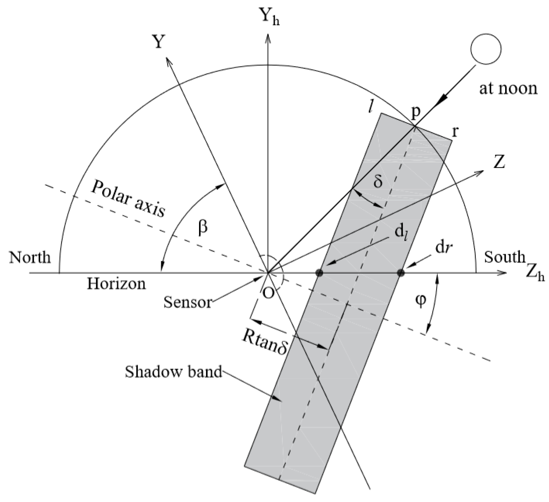
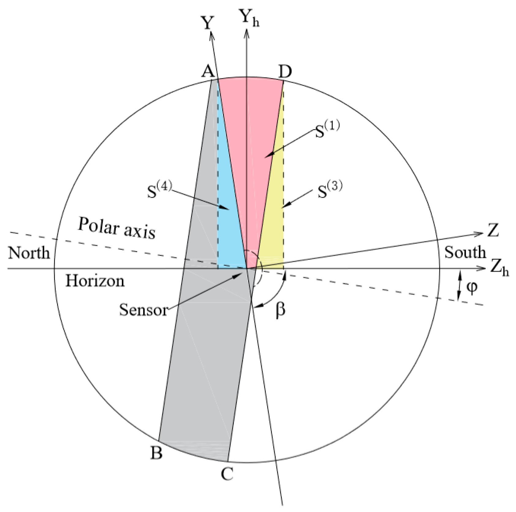
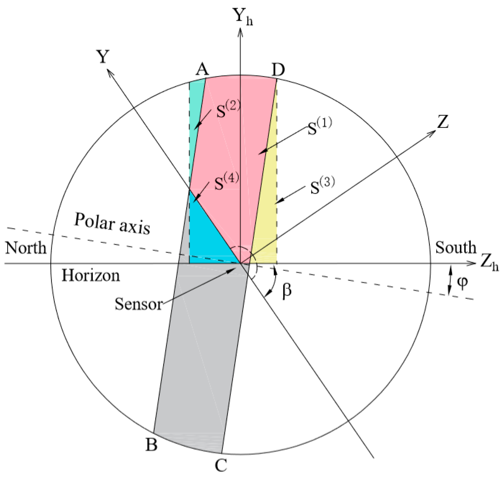
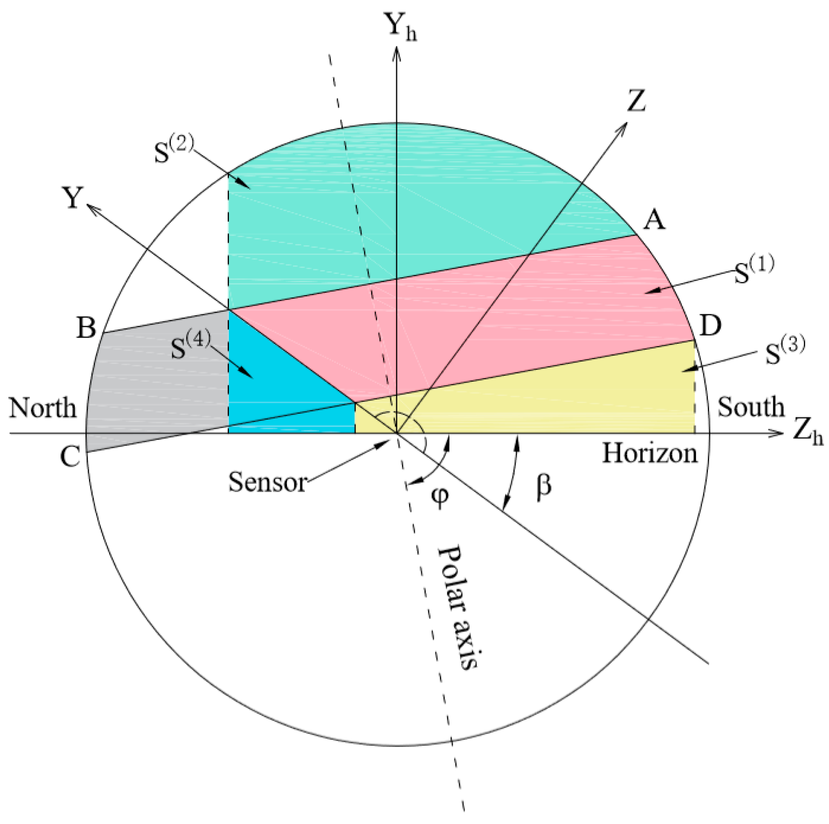
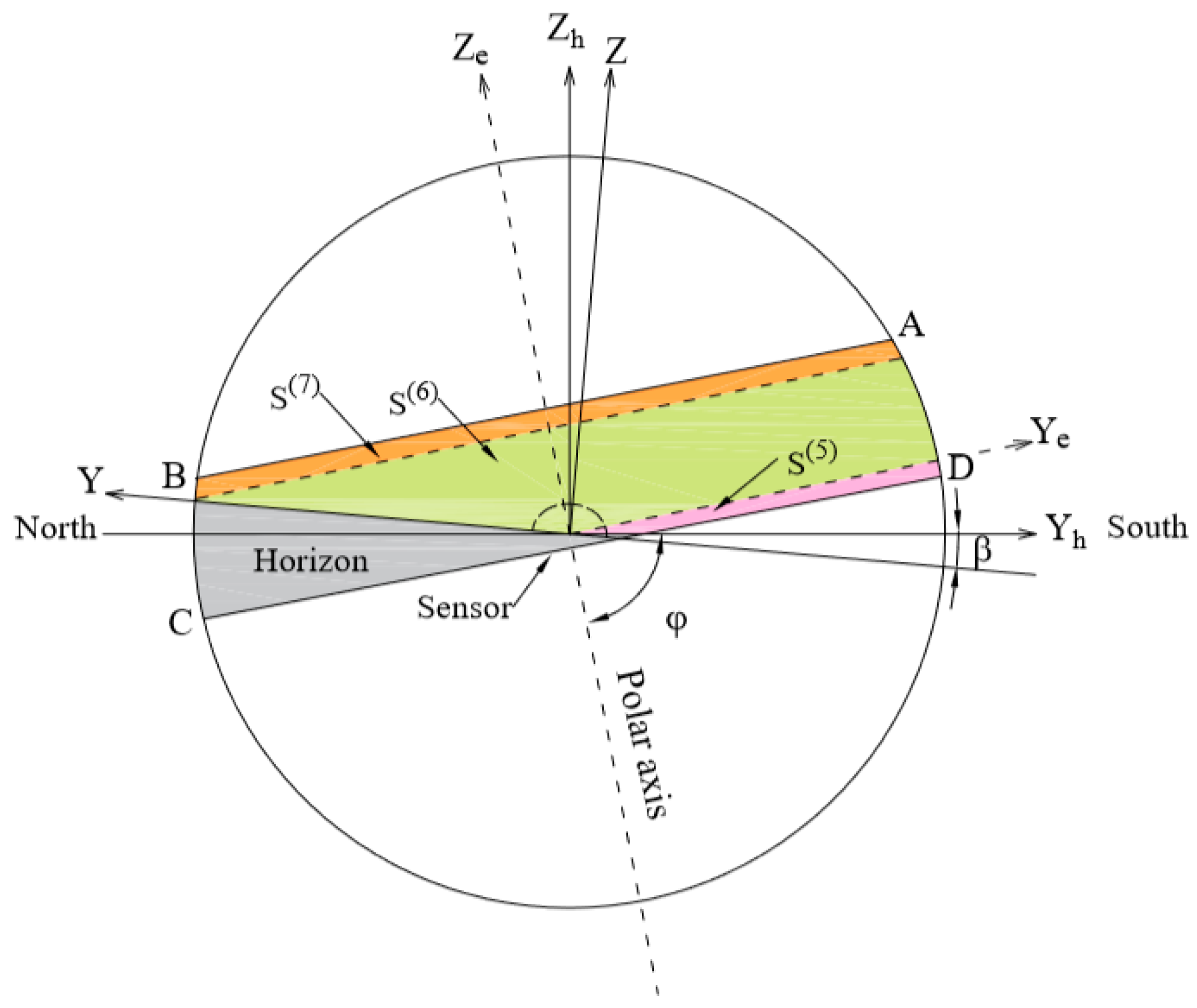
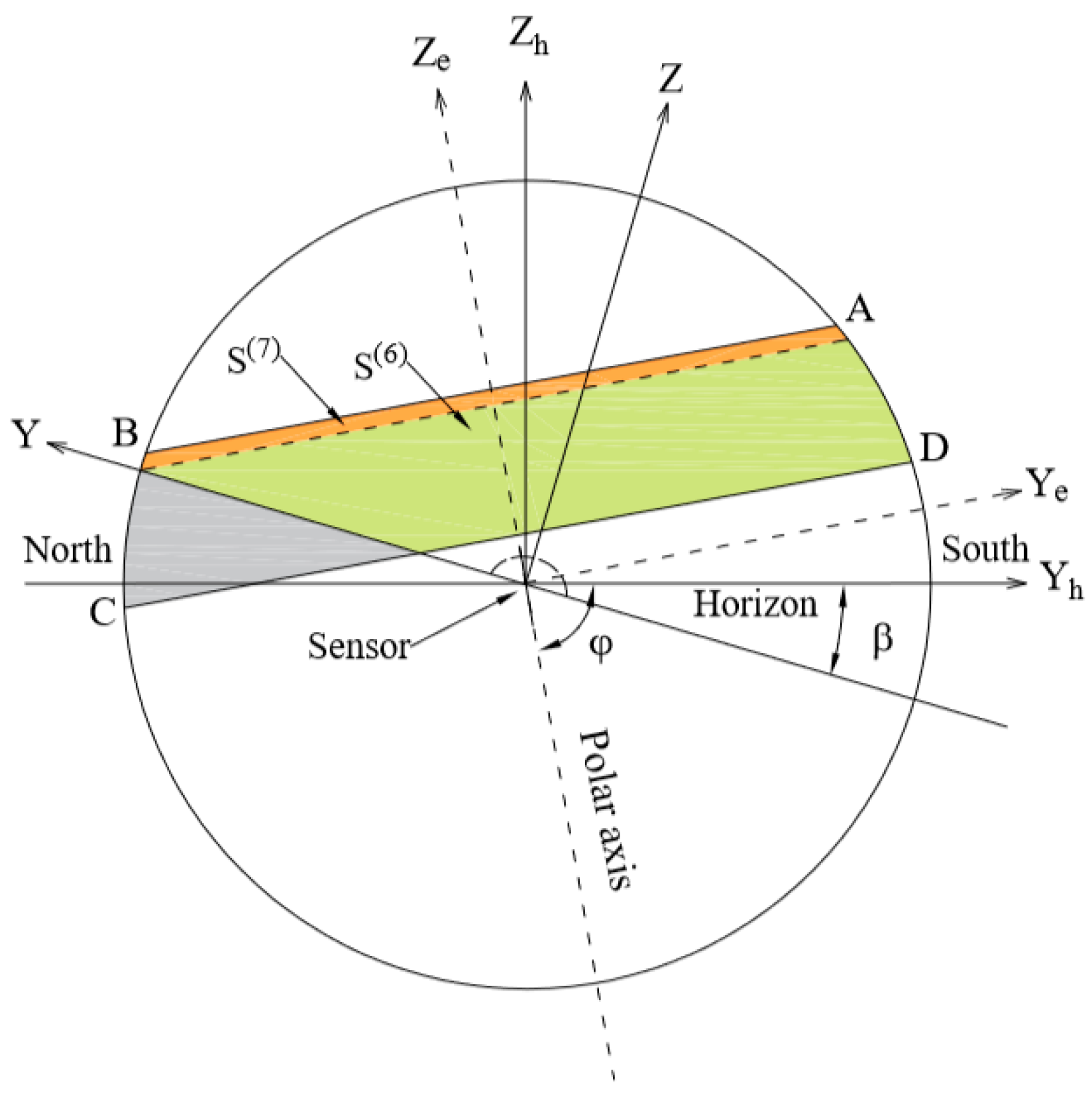
(1) The area S in Equation (1) and in the horizon coordinate system shown as Figure 1 at $\delta =0$ and $\phi =0$ is easily obtained and calculated by Equation (5). In the other situations shown as Figure 2 at $\delta \ne 0$ and $\phi \ne 0$, the area S can be calculated by the equations that are achieved by coordinate rotations and translations on the basis of Equation (5). However, all possibilities have to be considered and discussed.

Figure 1. Diagram of shadow band placement in the horizontal coordinate system at $\delta =0$ and $\phi =0$.

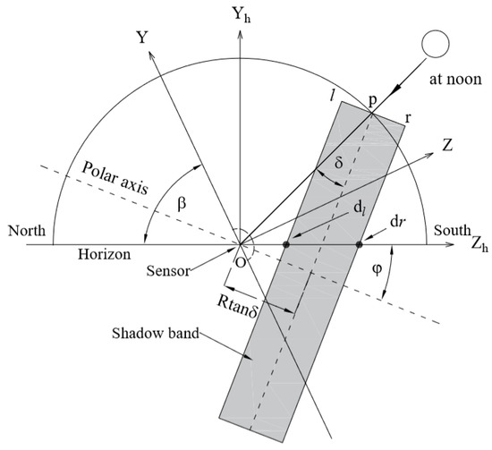
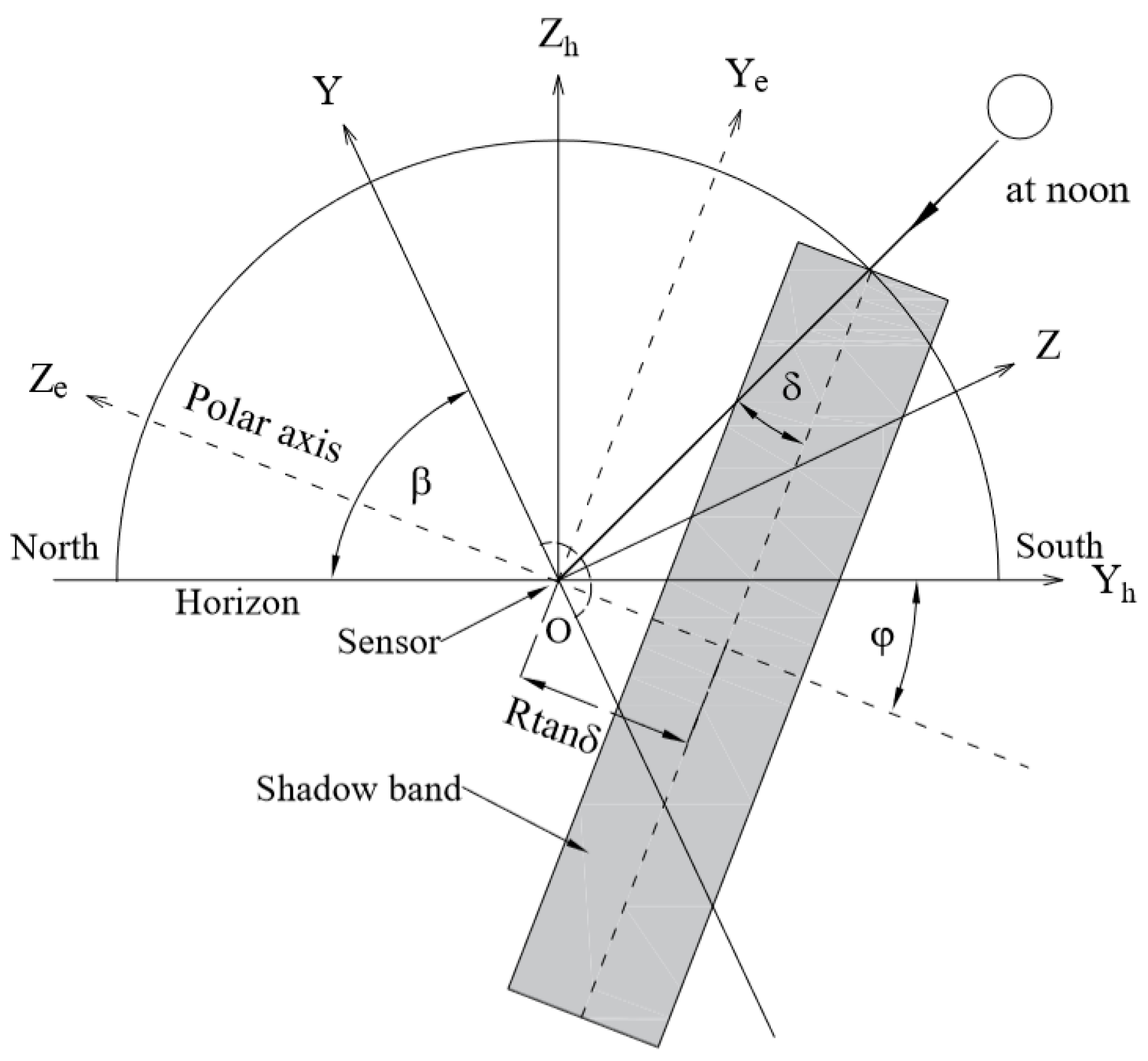
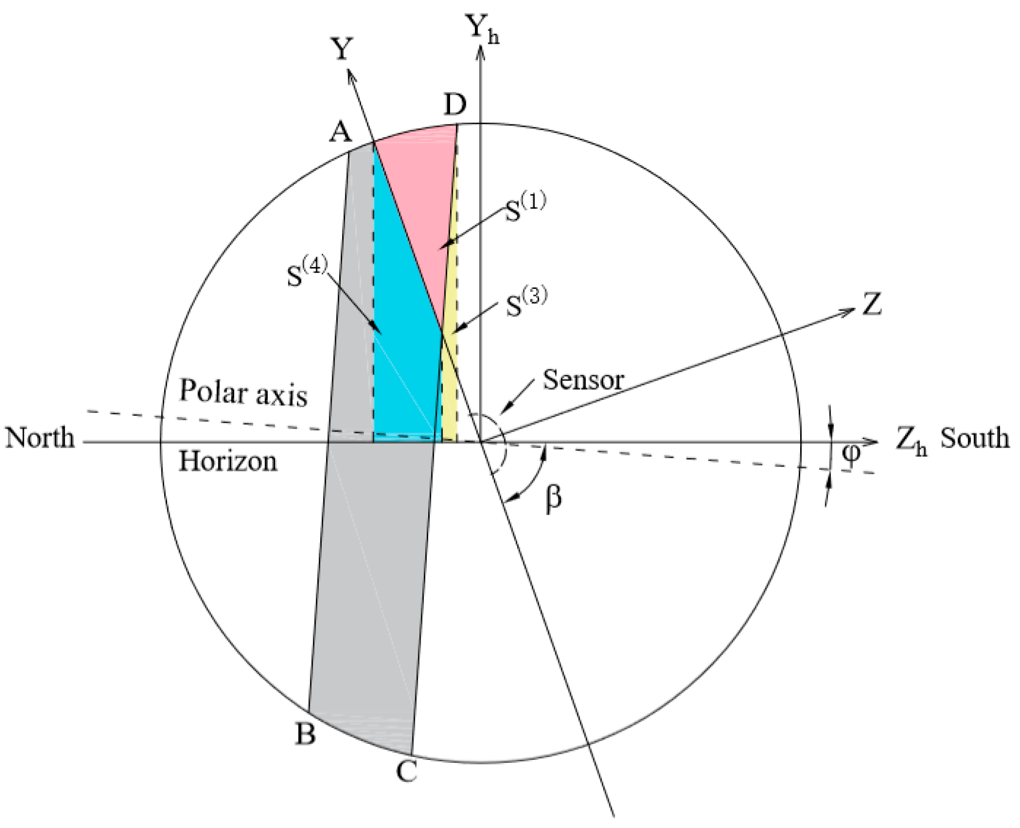
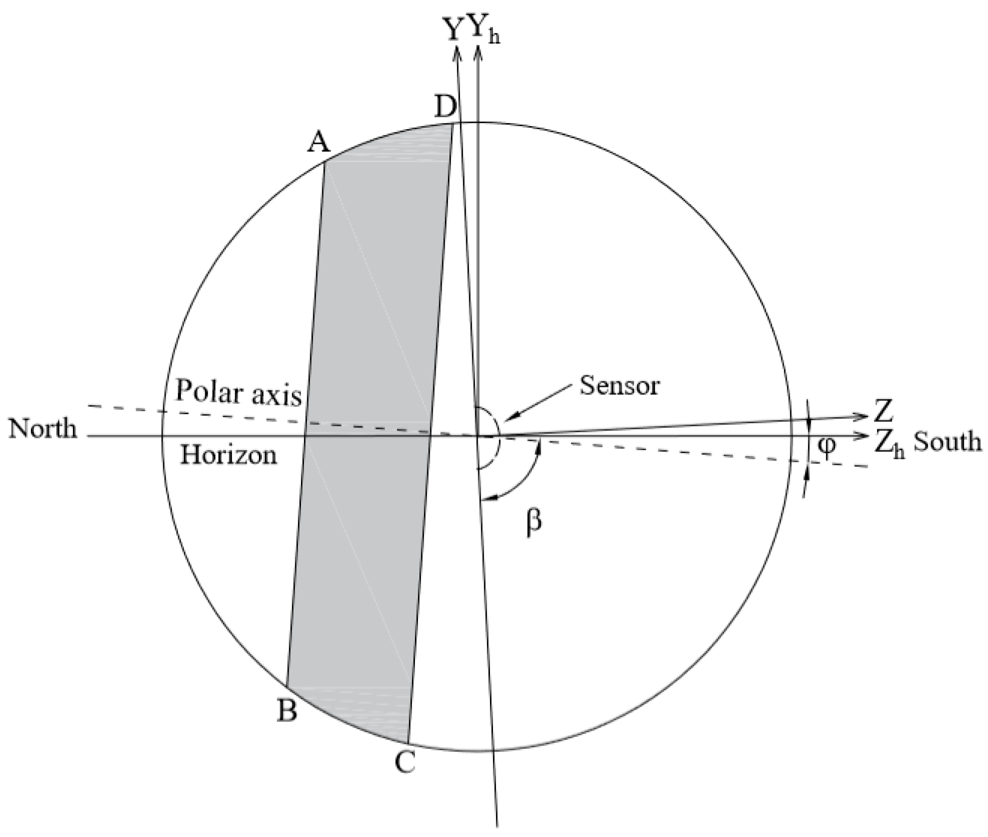
Figure 2. Diagram of shadow band placement in the horizontal coordinate system at $\delta \ne 0$ and $\phi \ne 0$.

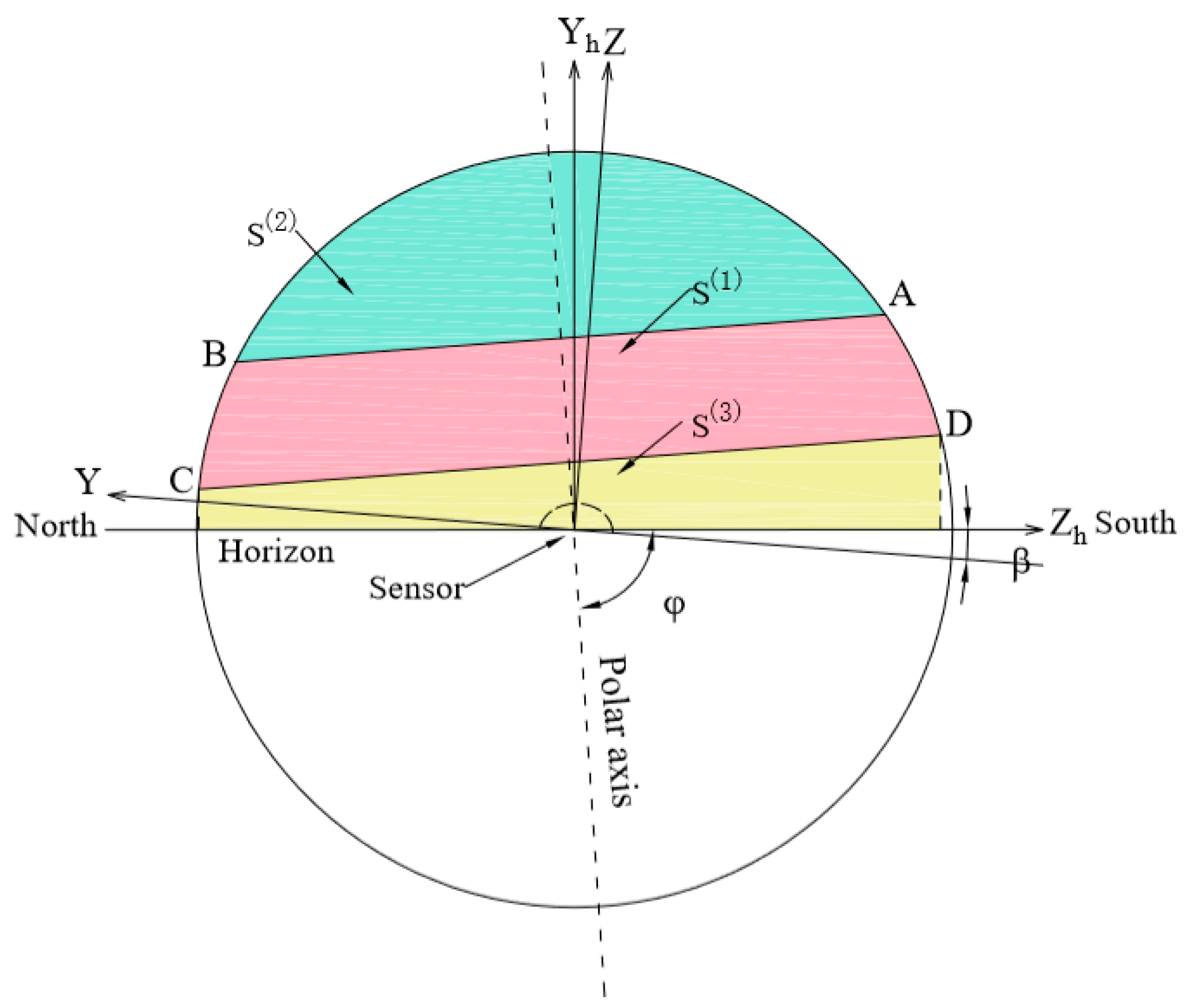
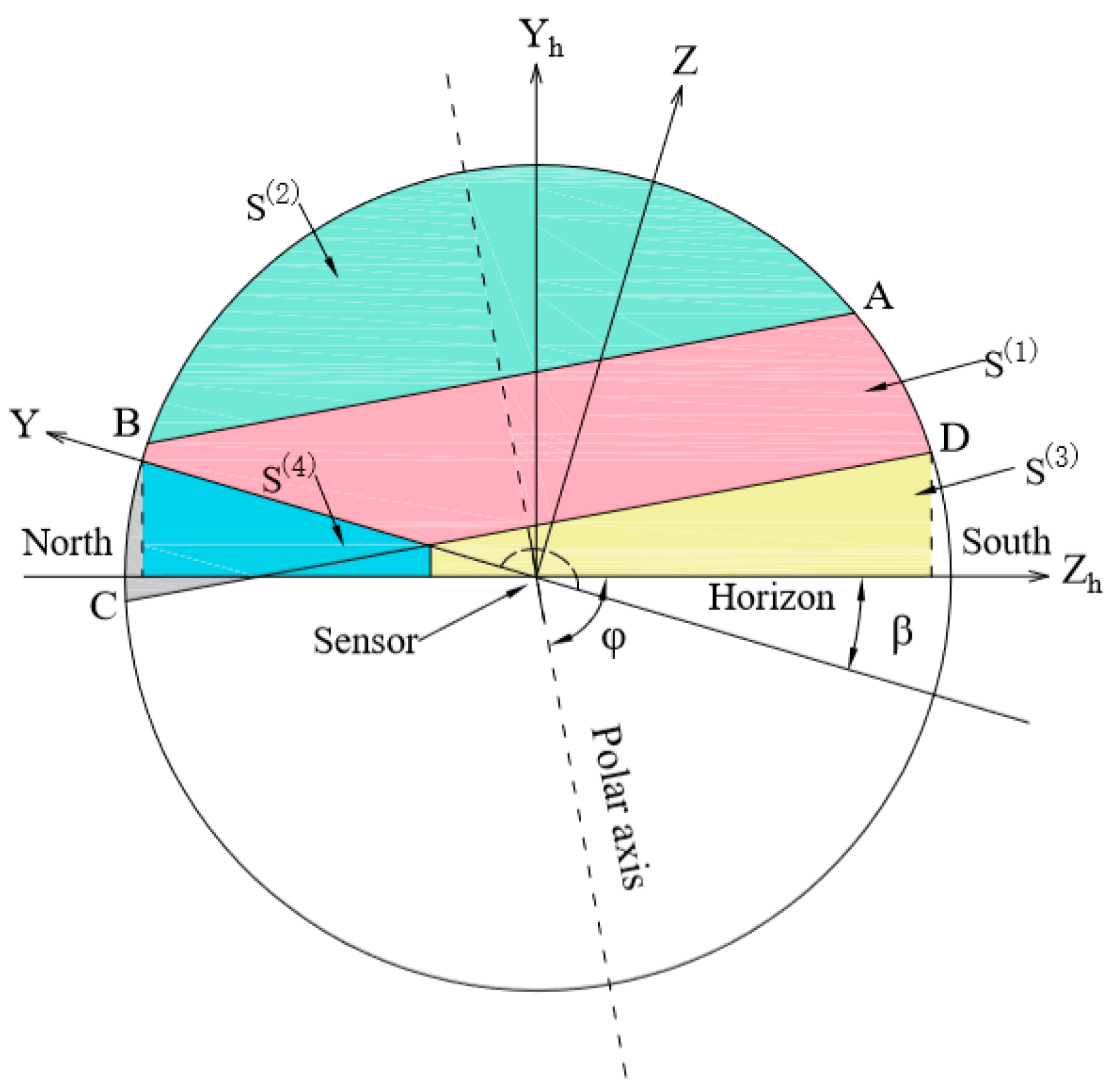
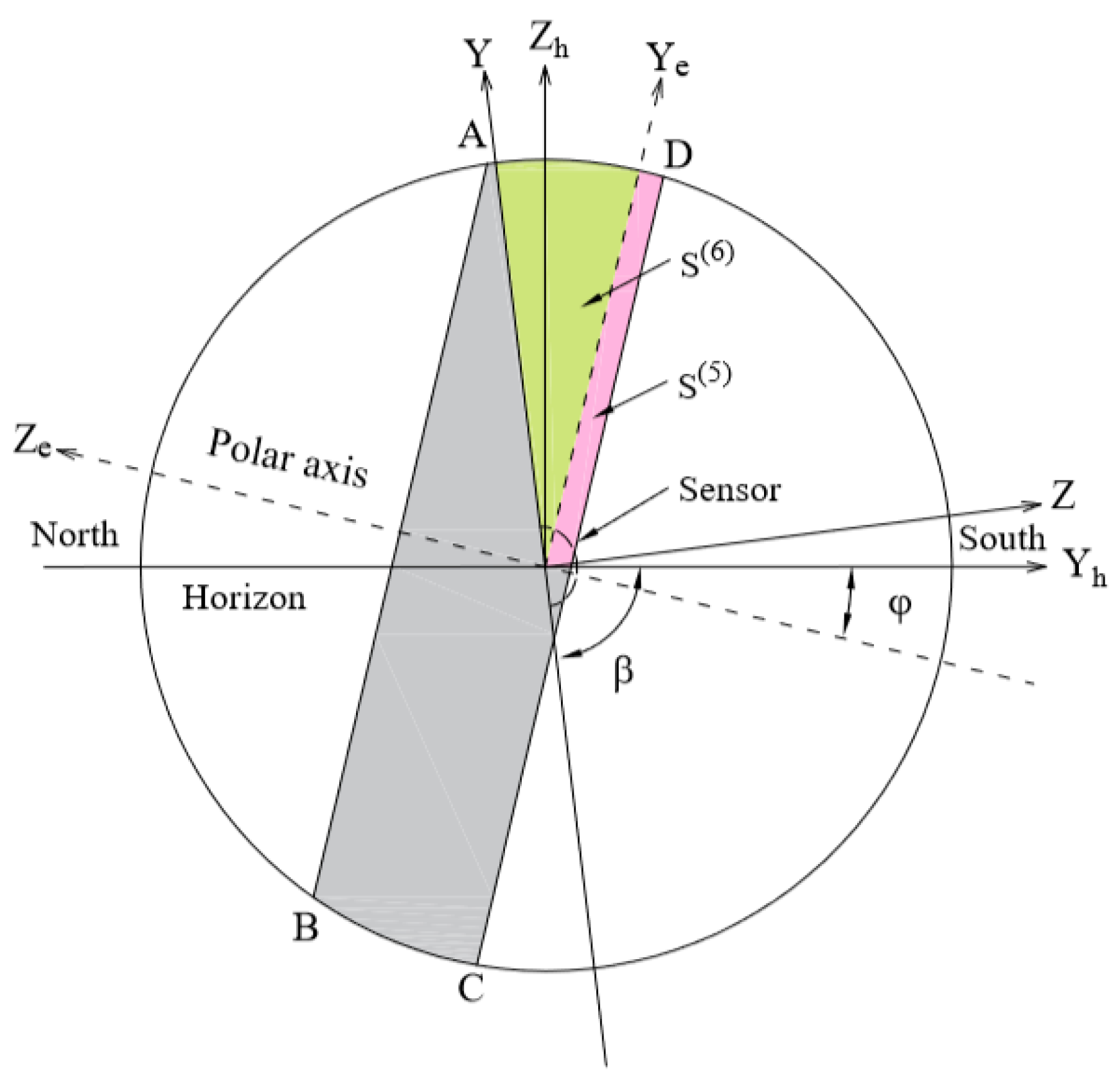
(2) The area S in Equation (1) and in the equatorial coordinate system shown as in Figure 3 at $\delta =0$ is easily obtained and calculated by Equation (43). In the other situations shown as Figure 4 at $\delta \ne 0$, the area S can be calculated by coordinate translations. However, all possibilities have to be considered and discussed.

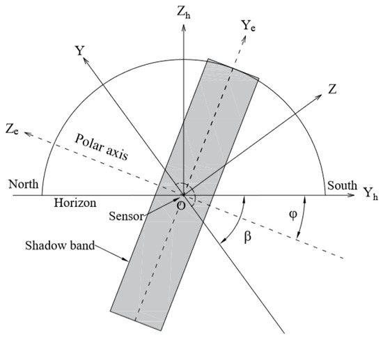
Figure 3. Diagram of shadow band placement in the equatorial coordinate system at $\delta =0$.

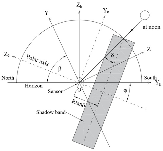
Figure 4. Diagram of shadow band placement in the equatorial coordinate system at $\delta \ne 0$.

(3) In order to avoid the risk of mistakes appeared during the calculation, the numerical evaluations of S and H in Equation (1) are carried out by coordinate transformations in different coordinate systems. Their results will be compared with each other and should be equal.

2.1. Discussions in Horizon Coordinate System

The Equation (1) in horizon coordinates will become

$$C_h=\frac{1}{\left(1-S_h/H_h\right)}$$

(2)

2.1.1. Calculation of $S_h$

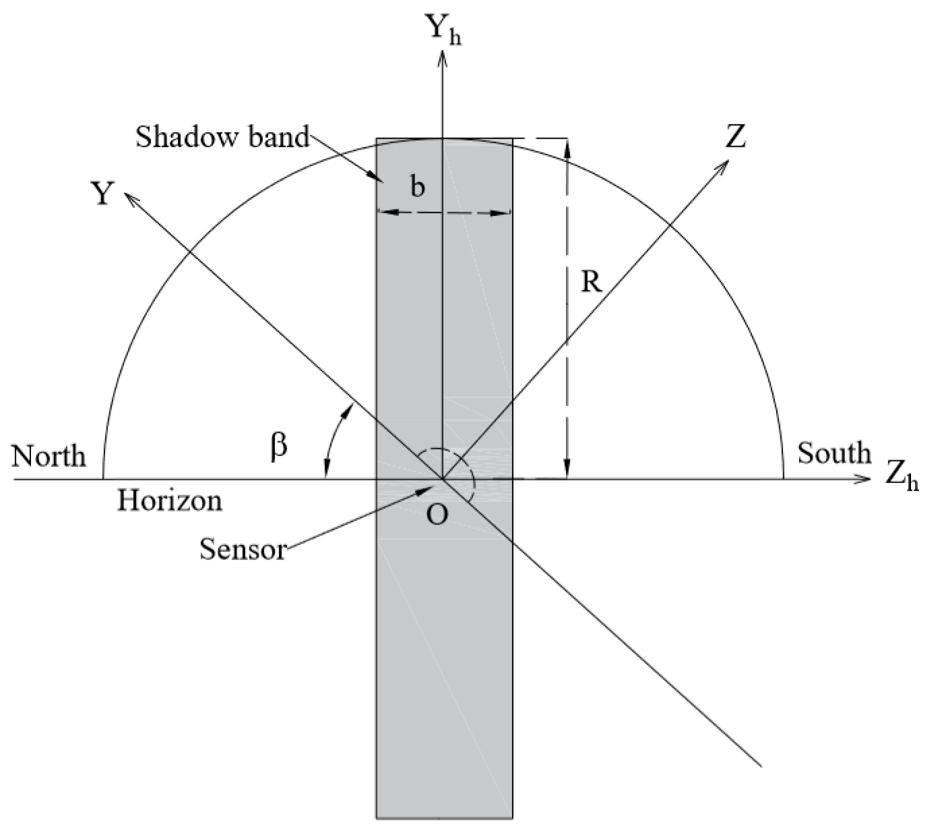
While the center of a shadow band is supposed to be coincided with the origin of horizon coordinate system and the radiation sensor is placed horizontally at $\delta =0$ and $\phi =0$, the shadow band should be put in the position shown as Figure 1. The equations of the spherical surface shaded by the shadow band in horizon coordinate system can be expressed as

$$\{\begin{array}{c}{x}_{h,0}{}^2+y_{h,0}{}^2+z_{h,0}{}^2={\mathrm{r}}^2\\ -\frac{bR}{\sqrt{b^2+4R^2}}\le z_{h,0}\le \frac{bR}{\sqrt{b^2+4R^2}}\end{array}$$

(3)

If the center of one sphere is coincided with the origin of horizon coordinates and the spherical surface is tangent to the surface of the shadow band, the radii of the sphere and the shadow band have the following correlation:

$$r=\frac{R_{ }}{\cos \left(\delta \right)}$$

(4)

As shown in Figure 1, the area $S_h$ projected onto the radiation sensor from the sky sphere and shaded by a shadow band can be calculated by

$$S_h={{\displaystyle \int }}_{{\alpha }_1}^{{\alpha }_2}{{\displaystyle \int }}_{{\varphi }_1}^{{\varphi }_2}{ℱ}_{h}d\varphi d\alpha$$

(5)

in which

$${ℱ}_h=\sin \left(\varphi \right)\left[\sin \left(\varphi \right)\sin \left(\alpha \right)\cos \left(\beta \right)+\cos \left(\varphi \right)\sin \left(\beta \right)\right]$$

(6)

While the sensor is put on a slope surface at the conditions of $\delta \ne 0$ and $\phi \ne 0$, the shadow band is placed in the position shown as Figure 2. The shadow band in Figure 2 can be considered as the result by rotating the shadow band in Figure 1 with an angle of $\phi$ around the axis of $X_h$ and then moving a distance of $R\tan \left(\delta \right)$ along the polar axis. Mathematically, it means that the shadow band in Figure 2 can be taken as the result of the shadow band in Figure 1 by coordinate transformations. $\left(x_h, y_h, z_h\right)$ are the coordinates of a point on the surface of the shadow band in Figure 2 and are supposed to be obtained by coordinate transformations of the point $\left(x_{h,0}, y_{h,0}, z_{h,0}\right)$ in Figure 1. The coordinate transformations are expressed as

$$\left[\begin{array}{c}{x}_h\\ y_{h }\\ z_h\\ 1\end{array}\right]=\left[\begin{array}{cccc}1& 0& 0& 0\\ 0& \cos \left(\phi \right)& -\sin \left(\phi \right)& 0\\ 0& \sin \left(\phi \right)& \cos \left(\phi \right)& 0\\ 0& 0& 0& 1\end{array}\right]\left[\begin{array}{c}{x}_{h,0}\\ y_{h,0}\\ z_{h,0}\\ 1\end{array}\right]+\left[\begin{array}{c}0\\ R\tan \left(\delta \right)\sin \left(\phi \right)\\ -R\tan \left(\delta \right)\cos \left(\phi \right)\\ 1\end{array}\right]$$

$$=\left[\begin{array}{c}{x}_{h,0}\\ y_{h,0}\cos \left(\phi \right)-z_{h,0}\sin \left(\phi \right)+R\tan \left(\delta \right)\sin \left(\phi \right)\\ y_{h,0}\sin \left(\phi \right)+z_{h,0}\cos \left(\phi \right)-R\tan \left(\delta \right)\cos \left(\phi \right)\\ 1\end{array}\right]$$

(7)

Then, we have

$$\{\begin{array}{l}{x}_h=x_{h,0}\\ y_h=y_{h,0}\cos \left(\phi \right)-z_{h,0}\sin \left(\phi \right)+R\tan \left(\delta \right)\sin \left(\phi \right)\\ z_h=y_{h,0}\sin \left(\phi \right)+z_{h,0}\cos \left(\phi \right)-R\tan \left(\delta \right)\cos \left(\phi \right)\end{array}$$

(8)

Before discussing $S_h$, the calculations of the angles of ${\gamma }_l$ and ${\gamma }_r$ are considered. As shown in Figure 2, the shadow band intersects the coordinate plane ${\mathrm{Y}}_{\mathrm{h}}{\mathrm{OZ}}_{\mathrm{h}}$ at the line segment $\overline{lr}$. ${\gamma }_l$ and ${\gamma }_r$ are the angles of two equal line segments of $\overline{lp}$ and $\overline{pr}$, respectively, about the origin O in the plane of ${\mathrm{Y}}_{\mathrm{h}}{\mathrm{OZ}}_{\mathrm{h}}$, and they can be calculated by

$${\gamma }_l={\cos }^{-1}\left\{\frac{2r+b\sin \left(\delta \right)}{2\sqrt{R^2+{\left[\frac{b}{2}+R\tan \left(\delta \right)\right]}^2}}\right\}$$

(9)

$${\gamma }_r={\cos }^{-1}\left\{\frac{2r-b\sin \left(\delta \right)}{2\sqrt{R_{ }{}^2+{\left[R\tan \left(\delta \right)-\frac{b}{2}\right]}^2}}\right\}$$

(10)

The calculations of $d_l$ and $d_r$ are also considered. They are $Z_h$ components of the coordinates of the intersections of left and right boundary planes of the shadow band with the axis $Z_h$, respectively, and are shown in Figure 2. They can be given by

$$d_l=r\cos \left(\frac{\pi }{2}-\phi +\delta +{\gamma }_l \right)-r\sin \left(\frac{\pi }{2}-\phi +\delta +{\gamma }_l\right)\tan \left(\phi \right)$$

(11)

$$d_r=r\cos \left(\frac{\pi }{2}-\phi +\delta -{\gamma }_r\right)-r\sin \left(\frac{\pi }{2}-\phi +\delta -{\gamma }_r\right)\tan \left(\phi \right)$$

(12)

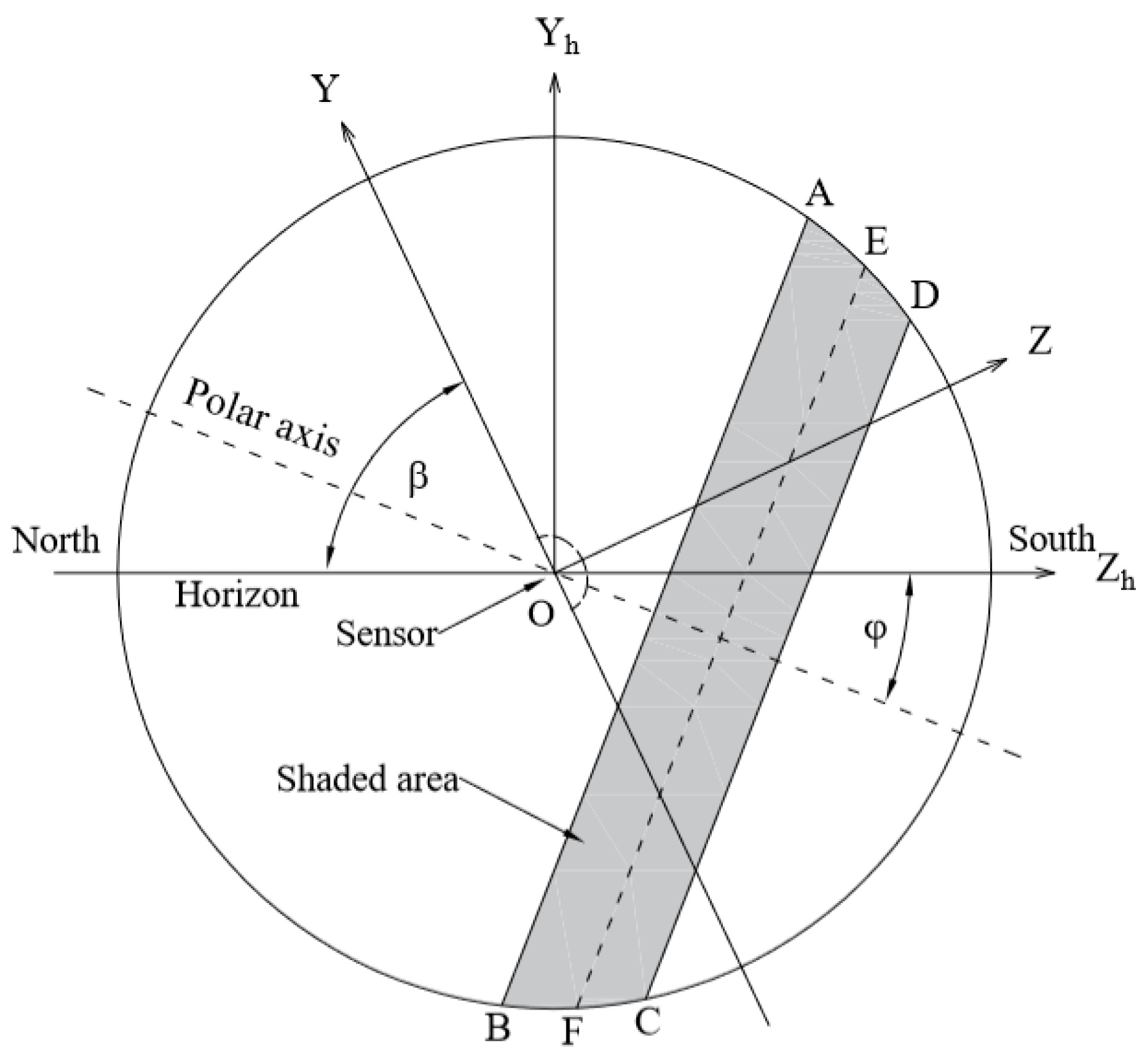
As shown in Figure 5, the area ABCD is projected by the spherical area, which is shaded by the shadow band, on the plane of ${\mathrm{Y}}_{\mathrm{h}}{\mathrm{OZ}}_{\mathrm{h}}$. E and F are the central points of the arcs AD and BC. It is obvious that the coordinates of the points E and F before the coordinate transformations are (0, R, 0) and (0, −R, 0) respectively. The coordinates ($x_{h,E}$, $y_{h,E}$, $z_{h,E}$) and ($x_{h,F}$, $y_{h,F}$, $z_{h,F}$) of the points E and F after coordinate transformations in the plane of ${\mathrm{Y}}_{\mathrm{h}}{\mathrm{OZ}}_{\mathrm{h}}$ are calculated by

$$\{\begin{array}{c}{y}_{h,E}=R\cos \left(\phi \right)+R\tan \left(\delta \right)\sin \left(\phi \right)\\ z_{h,E}=R\sin \left(\phi \right)-R\tan \left(\delta \right)\cos \left(\phi \right)\end{array}$$

(13)

$$\{\begin{array}{c}{y}_{h,F}=-R\cos \left(\phi \right)+R\tan \left(\delta \right)\sin \left(\phi \right)\\ z_{h,F}=-R\sin \left(\phi \right)-R\tan \left(\delta \right)\cos \left(\phi \right)\end{array}$$

(14)

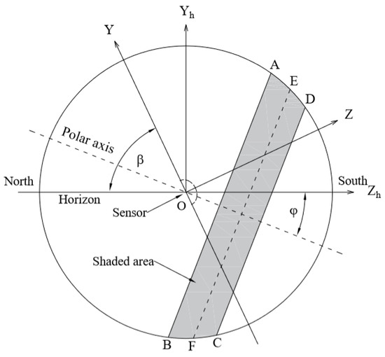
Figure 5. Spherical area shaded by a shadow band and projected on the plane ${\mathrm{Y}}_{\mathrm{h}}{\mathrm{OZ}}_{\mathrm{h}}$ while $d_l\ge 0$.

Let ($x_{h, A}$, $y_{h,A}$, $z_{h,A}$) and ($x_{h, B}$, $y_{h,B}$, $z_{h,B}$) represent the coordinates of the points A and B in Figure 5. Then, the coordinates in the plane of ${\mathrm{Y}}_{\mathrm{h}}{\mathrm{OZ}}_{\mathrm{h}}$ can be obtained by

$$\{\begin{array}{c}{y}_{h,A}=r\cos \left[{\tan }^{-1}\left(\frac{z_{h,E}}{y_{h,E}}\right)-{\gamma }_l\right]\\ z_{h,A}=r\sin \left[{\tan }^{-1}\left(\frac{z_{h,E}}{y_{h,E}}\right)-{\gamma }_l\right]\end{array}$$

(15)

$$\{\begin{array}{c}{y}_{h,B}=r\cos \left[{\tan }^{-1}\left(\frac{z_{h,F}}{y_{h,F}}\right)+{\gamma }_l\right]\\ z_{h,B}=r\sin \left[{\tan }^{-1}\left(\frac{z_{h,F}}{y_{h,F}}\right)+{\gamma }_l\right]\end{array}$$

(16)

Furthermore, the minimum and the maximum of the angles $\varphi$ of all points of the left boundary curve of the spherical area shaded by the shadow band above the horizontal plane are

$${\varphi }_{h,l,min}=\{\begin{array}{c}{\cos }^{-1}\left[\sin \left(\phi -\delta -{\gamma }_l\right)\right] y_{h,A}>0 \\ 0 y_{h,A}\le 0 \end{array}$$

(17)

$${\varphi }_{h,l,max}=\{\begin{array}{c} {\cos }^{-1}\left(\frac{d_l}{r}\right) y_{h,B}<0 and y_{h,A}>0\\ {\cos }^{-1}\left[\sin \left(\pi +\phi +\delta +{\gamma }_l\right)\right] y_{h,B}\ge 0 and y_{h,A}>0 \\ 0 y_{h,A}\le 0 \end{array}$$

(18)

Similarly, let ($x_{h, C}$, $y_{h,C}$, $z_{h,C}$) and ($x_{h, D}$, $y_{h,D}$, $z_{h,D}$) represent the coordinates of the points C and D. Their coordinates in the plane of ${\mathrm{Y}}_{\mathrm{h}}{\mathrm{OZ}}_{\mathrm{h}}$ can be achieved by

$$\{\begin{array}{c}{y}_{h,D}=r\cos \left[{\tan }^{-1}\left(\frac{z_{h,E}}{y_{h,E}}\right)+{\gamma }_r\right]\\ z_{h,D}=r\sin \left[{\tan }^{-1}\left(\frac{z_{h,E}}{y_{h,E}}\right)+{\gamma }_r\right]\end{array}$$

(19)

$$\{\begin{array}{c}{y}_{h,C}=r\cos \left[{\tan }^{-1}\left(\frac{z_{h,F}}{y_{h,F}}\right)-{\gamma }_r\right]\\ z_{h,C}=r\sin \left[{\tan }^{-1}\left(\frac{z_{h,F}}{y_{h,F}}\right)-{\gamma }_r\right]\end{array}$$

(20)

The minimum and the maximum of the angles $\varphi$ of all points of the right boundary curve of the spherical area shaded by the shadow band above the horizontal plane are

$${\varphi }_{h,r,min}=\{\begin{array}{c}{\cos }^{-1}\left[\sin \left(\phi -\delta +{\gamma }_r\right)\right] y_{h,D}>0 \\ 0 y_{h,D}\le 0 \end{array}$$

(21)

$${\varphi }_{h,r,max}=\{\begin{array}{c} {\cos }^{-1}\left(\frac{d_r}{r}\right) y_{h,C}<0 and y_{h,D}>0\\ {\cos }^{-1}\left[\sin \left(\pi +\phi +\delta -{\gamma }_r\right)\right] y_{h,C}\ge 0 and y_{h,D}>0\\ 0 y_{h,D}\le 0 \end{array}$$

(22)

Due to the shadow band positions decided by $\delta$, $\phi$ and $\beta$, the formula of (5) will have different types of expressions. All possibilities of the expressions are discussed as following:

(1) While $d_l\ge 0$, as shown as Figure 6, $S^{\left(1\right)}$ is the area, which is projected by the spherical area $S_h$ on the plane ${\mathrm{Y}}_{\mathrm{h}}{\mathrm{OZ}}_{\mathrm{h}}$, and will continually be used to represent the area in the following discussions. Then, the Equation (5) can be written as:

$$S_h={{\displaystyle \int }}_0^{\pi }{{\displaystyle \int }}_{{\varphi }_{h,r,min}}^{{\varphi }_{h,l,max}}{ℱ}_{h}d\varphi d\alpha -{{\displaystyle \int }}_{{\alpha }_{h,l,1}}^{{\alpha }_{h,l,2}}{{\displaystyle \int }}_{{\varphi }_{h,l,min}}^{{\varphi }_{h,l,max}}{ℱ}_{h}d\varphi d\alpha -2{{\displaystyle \int }}_0^{{\alpha }_{h,r,1}}{{\displaystyle \int }}_{{\varphi }_{h,r,min}}^{{\varphi }_{h,r,max}}{ℱ}_{h}d\varphi d\alpha$$

(23)

in which

$${\alpha }_{h,l,1}={\sin }^{-1}\left[\frac{\cos \left(\varphi \right)-d_l/r}{\sin \left(\varphi \right)\tan \left(\phi \right)}\right]$$

(24)

$${\alpha }_{h,l,2}=\pi -{\alpha }_{h,l,1}$$

(25)

$${\alpha }_{h,r,1}={\sin }^{-1}\left[\frac{\cos \left(\varphi \right)-d_r/r}{\sin \left(\varphi \right)\tan \left(\phi \right)}\right]$$

(26)

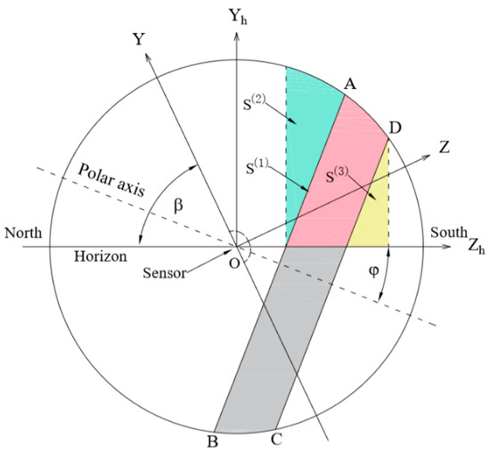
Figure 6. Schematic diagram for the integration of $S_h$ while $d_l\ge 0$.

$S^{\left(2\right)}$ and $S^{\left(3\right)}$ are the areas that are projected on the plane ${\mathrm{Y}}_{\mathrm{h}}{\mathrm{OZ}}_{\mathrm{h}}$ by the spherical areas and will be used to represent the areas in the following discussions. Those spherical areas are above the left boundary section and below the right boundary section of the shadow band, respectively. the spherical areas are calculated by the second and the third terms on the right-hand side of Equation (23).

(2) While $d_l<0<d_r$ and ${\varphi }_{h,l,min}>\pi -\beta$, shown as Figure 7, the axis Y is between the points A and D. The Equation (5) is written as

$$S_h={{\displaystyle \int }}_0^{\pi }{{\displaystyle \int }}_{{\varphi }_{h,r,min}}^{\pi -\beta }{ℱ}_{h}d\varphi d\alpha -2{{\displaystyle \int }}_0^{{\alpha }_{h,r,1}}{{\displaystyle \int }}_{{\varphi }_{h,r,min}}^{{\varphi }_{h,r,max}}{ℱ}_{h}d\varphi d\alpha -2{{\displaystyle \int }}_0^{{\alpha }_{h,i,1}}{{\displaystyle \int }}_{\frac{\pi }{2}}^{\pi -\beta }{ℱ}_{h}d\varphi d\alpha$$

(27)

in which

$${\alpha }_{h,i,1}={\sin }^{-1}\left[-\cot \left(\varphi \right)\tan \left(\beta \right)\right]$$

(28)

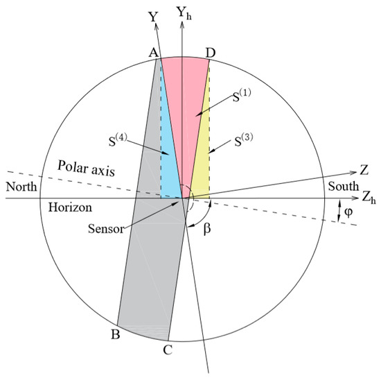
Figure 7. Schematic diagram for the calculation of $S_h$ while $d_l<0<d_r$ and ${\varphi }_{h,l,min}>\pi -\beta$.

$S^{\left(4\right)}$ is the area, which is projected on the plane ${\mathrm{Y}}_{\mathrm{h}}{\mathrm{OZ}}_{\mathrm{h}}$ by the spherical area below the slope surface, and will be used to represent the area in the following discussions. The spherical area is calculated by the third term on the right-hand side of Equation (27).

(3) While $d_l<0<d_r$ and ${\varphi }_{h,l,max}\ge {\varphi }_{h,l{\displaystyle \cap }i}\ge {\varphi }_{h,l,min}$, shown as Figure 8, the axis Y is between the points A and B. $S_h$ can be calculated by

$$\begin{gathered} S_h={{\displaystyle \int }}_0^{\pi }{{\displaystyle \int }}_{{\varphi }_{h,r,min}}^{{\varphi }_{h,l{\displaystyle \cap }i}}{ℱ}_{h}d\varphi d\alpha -{{\displaystyle \int }}_{{\alpha }_{h,l,1}}^{{\alpha }_{h,l,2}}{{\displaystyle \int }}_{{\varphi }_{h,l,min}}^{{\varphi }_{h,l{\displaystyle \cap }i}} {ℱ}_{h}d\varphi d\alpha \\ -2{{\displaystyle \int }}_0^{{\alpha }_{h,r,1}}{{\displaystyle \int }}_{{\varphi }_{h,r,min}}^{{\varphi }_{h,r,max}}{ℱ}_{h}d\varphi d\alpha \\ -2{{\displaystyle \int }}_0^{{\alpha }_{h,i,1}}{{\displaystyle \int }}_{\frac{\pi }{2}}^{{\varphi }_{h,l{\displaystyle \cap }i}}{ℱ}_{h}d\varphi d\alpha \end{gathered}$$

(29)

in which

$${\varphi }_{h,l{\displaystyle \cap }i}={\cos }^{-1}\left[\frac{d_l}{r\left(1+\tan \left(\phi \right)\tan \left(\beta \right)\right)}\right]$$

(30)

Figure 8. Schematic diagram for the calculation of $S_h$ while $d_l<0<d_r$ and ${\varphi }_{h,l,max}\ge {\varphi }_{h,l{\displaystyle \cap }i}\ge {\varphi }_{h,l,min}$.

(4) while $d_l<0<d_r$, $y_{h,B}>0$ and ${\varphi }_{h,l,max}<\pi -\beta$, shown as in Figure 9, the axis Y is between the points B and C. The Equation (5) can be written as

$$\begin{gathered} {\mathrm{S}}_{\mathrm{h}}={{\displaystyle \int }}_0^{\pi }{{\displaystyle \int }}_{{\varphi }_{h,r,min}}^{\pi -\beta }{ℱ}_{h}d\varphi d\alpha -{{\displaystyle \int }}_{{\alpha }_{h,l,1}}^{{\alpha }_{h,l,2}}{{\displaystyle \int }}_{{\varphi }_{h,l,min}}^{{\varphi }_{h,l,max}}{ℱ}_{h}d\varphi d\alpha -2{{\displaystyle \int }}_0^{{\alpha }_{h,r,1}}{{\displaystyle \int }}_{{\varphi }_{h,r,min}}^{{\varphi }_{h,r,max}}{ℱ}_{h}d\varphi d\alpha \\ -2{{\displaystyle \int }}_0^{{\alpha }_{h,i,1}}{{\displaystyle \int }}_{\frac{\pi }{2}}^{\pi -\beta }{ℱ}_{h}d\varphi d\alpha \end{gathered}$$

(31)

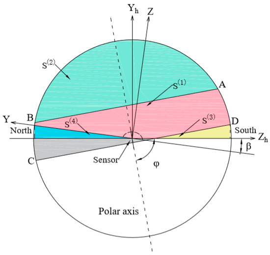
Figure 9. Schematic diagram for the calculation of $S_h$ while $d_l<0<d_r$, $y_{h,B}>0$ and ${\varphi }_{h,l,max}<\pi -\beta$.

(5) while $d_r\le 0$, $y_{h,C}>0$ and ${\varphi }_{h,r,max}<\pi -\beta$, shown as in Figure 10, the axis Y is below the point C. $S_h$ can be calculated by

$$S_h={{\displaystyle \int }}_0^{\pi }{{\displaystyle \int }}_{{\varphi }_{h,r,min}}^{{\varphi }_{h,r,max}}{ℱ}_{h}d\varphi d\alpha -{{\displaystyle \int }}_{{\alpha }_{h,l,1}}^{{\alpha }_{h,l,2}}{{\displaystyle \int }}_{{\varphi }_{h,l,min}}^{{\varphi }_{h,l,max}}{ℱ}_{h}d\varphi d\alpha -2{{\displaystyle \int }}_0^{{\alpha }_{h,r,1}}{{\displaystyle \int }}_{{\varphi }_{h,r,min}}^{{\varphi }_{h,r,max}} {ℱ}_{h}d\varphi d\alpha$$

(32)

Figure 10. Schematic diagram for the calculation of $S_h$ while $d_r\le 0$, $y_{h,C}>0$ and ${\varphi }_{h,r,max}<\pi -\beta$.

(6) while $d_r\le 0$, $y_{h,B}>0$ and ${\varphi }_{h,l,max}<\pi -\beta$, ${\varphi }_{h,r,max}\ge {\varphi }_{h,r{\displaystyle \cap }i}\ge {\varphi }_{h,r,min}$, shown as in Figure 11, the axis Y is between the points B and C. The Equation (5) can be written as

$$S_h={{\displaystyle \int }}_0^{\pi }{{\displaystyle \int }}_{{\varphi }_{h,r,min}}^{\pi -\beta }{ℱ}_{h}d\varphi d\alpha -{{\displaystyle \int }}_{{\alpha }_{h,l,1}}^{{\alpha }_{h,l,2}}{{\displaystyle \int }}_{{\varphi }_{h,l,min}}^{{\varphi }_{h,l,max}} {ℱ}_{h}d\varphi d\alpha -2{{\displaystyle \int }}_0^{{\alpha }_{h,r,1}}{{\displaystyle \int }}_{{\varphi }_{h,r,min}}^{{\varphi }_{h,r{\displaystyle \cap }i}}{ℱ}_{h}d\varphi d\alpha$$

$$-2{{\displaystyle \int }}_0^{{\alpha }_{h,i,1}}{{\displaystyle \int }}_{{\varphi }_{h,r{\displaystyle \cap }i}}^{\pi -\beta }{ℱ}_{h}d\varphi d\alpha$$

(33)

in which

$${\varphi }_{h,r{\displaystyle \cap }i}={\cos }^{-1}\left[\frac{d_r}{r\left(1+\tan \left(\phi \right)\tan \left(\beta \right)\right)}\right]$$

(34)

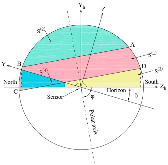
Figure 11. Schematic diagram for the calculation of $S_h$ while $d_r\le 0$, $y_{h,C}>0$ and ${\varphi }_{h,r,max}<\pi -\beta$, ${\varphi }_{h,r,max}\ge {\varphi }_{h,r{\displaystyle \cap }i}\ge {\varphi }_{h,r,min}$.

(7) While $d_r\le 0$, ${\varphi }_{h,l,max}\ge {\varphi }_{h,l{\displaystyle \cap }i}\ge {\varphi }_{h,l,min}, {\varphi }_{h,r,max}\ge {\varphi }_{h,r{\displaystyle \cap }i}\ge {\varphi }_{h,r,min},$ shown as Figure 12, the axis Y is between the points A and B. The Equation (5) can be written as

$$S_h={{\displaystyle \int }}_0^{\pi }{{\displaystyle \int }}_{{\varphi }_{h,r,min}}^{{\varphi }_{h,l{\displaystyle \cap }i}}{ℱ}_{h}d\varphi d\alpha -{{\displaystyle \int }}_{{\alpha }_{h,l,1}}^{{\alpha }_{h,l,2}}{{\displaystyle \int }}_{{\varphi }_{h,l,min}}^{{\varphi }_{h,l{\displaystyle \cap }i}}{ℱ}_{h,i}d\varphi d\alpha -2{{\displaystyle \int }}_0^{{\alpha }_{h,r,1}}{{\displaystyle \int }}_{{\varphi }_{h,r,min}}^{{\varphi }_{h,r{\displaystyle \cap }i}}{ℱ}_{h}d\varphi d\alpha$$

$$-2{{\displaystyle \int }}_0^{{\alpha }_{h,i,1}}{{\displaystyle \int }}_{{\varphi }_{h,r{\displaystyle \cap }i}}^{{\varphi }_{h,l{\displaystyle \cap }i}}{ℱ}_{h}d\varphi d\alpha$$

(35)

Figure 12. Schematic diagram for the calculation of $S_h$ while $d_r\le 0$, ${\varphi }_{h,l,max}\ge {\varphi }_{h,l{\displaystyle \cap }i}\ge {\varphi }_{h,l,min}, {\varphi }_{h,r,max}\ge {\varphi }_{h,r{\displaystyle \cap }i}\ge {\varphi }_{h,r,min}$.

(8) while $d_r\le 0$, ${\varphi }_{h,l,min}>\pi -\beta >{\varphi }_{h,r,min}$, shown as Figure 13, the axis Y is between the points A and D. The Equation (5) becomes

$$S_h={{\displaystyle \int }}_0^{\pi }{{\displaystyle \int }}_{{\varphi }_{h,r,min}}^{\pi -\beta }{ℱ}_{h}d\varphi d\alpha -2{{\displaystyle \int }}_0^{{\alpha }_{h,r,1}}{{\displaystyle \int }}_{{\varphi }_{h,r,min}}^{{\varphi }_{h,r{\displaystyle \cap }i}} {ℱ}_{h}d\varphi d\alpha -2{{\displaystyle \int }}_0^{{\alpha }_{h,i,1}}{{\displaystyle \int }}_{{\varphi }_{h,r{\displaystyle \cap }i}}^{\pi -\beta }{ℱ}_{h}d\varphi d\alpha$$

(36)

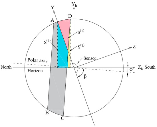
Figure 13. Schematic diagram for the calculation of $S_h$ while $d_r\le 0$ and ${\varphi }_{h,l,min}>\pi -\beta >{\varphi }_{h,r,min}$.

(9) while $d_r\le 0$, ${\varphi }_{h,r,min}>\pi -\beta$, shown as Figure 14, it is easily understood that the Equation (5) becomes

$$S_h=0$$

(37)

Figure 14. Schematic diagram for the calculation of $S_h$ while $d_r\le 0$ and ${\varphi }_{h,r,min}>\pi -\beta$.

2.1.2. Calculation of $H_h$

The area $H_{h,s}$ projected from the sky sphere onto the radiation sensor in horizon coordinates can be calculated by

$$H_{h,s}={{\displaystyle \int }}_0^{\pi }{{\displaystyle \int }}_0^{\frac{\pi }{2}}{ℱ}_{h}d\varphi d\alpha +{{\displaystyle \int }}_{{\alpha }_{h,i,1}}^{{\alpha }_{h,i,2}}{{\displaystyle \int }}_{\frac{\pi }{2}}^{\pi -\beta }{ℱ}_{h}d\varphi d\alpha$$

(38)

The precise calculation of the projected portion of the hemisphere curved surface area due to ground albedo in the horizon coordinates is discussed by Muhammad Iqbal [16] and it is

$$H_{h,g}=\rho \pi \frac{1-\cos \left(\beta \right)}{2}$$

(39)

Then, the area $H_h$ in Equation (2) is calculated by

$$H_h=H_{h,s}+H_{h,g}$$

(40)

2.2. Discussions in Equatorial Coordinate System

The Equation (1) in equatorial coordinates will become

$$C_e=\frac{1}{\left(1-S_e/H_e\right)}$$

(41)

2.2.1. Calculation of $S_e$

As shown in Figure 3, while the shadow band is perpendicular to polar axis and its center is supposed to be coincided with the origin of horizon coordinate system and equatorial coordinate system at $\delta =0$, the equations of the spherical surface shaded by the shadow band in equatorial coordinate system can be expressed as

$$\{\begin{array}{c}{x}_{e,0}{}^2+y_{e,0}{}^2+z_{e,0}{}^2=r^2\\ -\frac{bR}{\sqrt{b^2+4R^2}}\le z_{e,0}\le \frac{bR}{\sqrt{b^2+4R^2}}\end{array}$$

(42)

If one spherical center is coincided with the origin of equatorial coordinate system and the spherical surface is tangent to the surface of the shadow band, the correlation of the radius r of the sphere with the radius R of the shadow band is expressed as Equation (4). The area projected onto the radiation sensor from the sky sphere, which is shaded by a shadow band, in the equatorial coordinate system can be given by

$$S_e={{\displaystyle \int }}_{{\alpha }_1}^{{\alpha }_2}{{\displaystyle \int }}_{{\varphi }_1}^{{\varphi }_2}{ℱ}_{e}d\varphi d\alpha$$

(43)

in which

$${ℱ}_e=\sin \left(\varphi \right)\left[\sin \left(\varphi \right)\sin \left(\alpha \right)\cos \left(\phi -\beta \right)+\cos \left(\varphi \right)\sin \left(\phi -\beta \right)\right]$$

(44)

While $\delta \ne 0$ (the placement of the shadow band is shown in Figure 4) this can be the result of the shadow band shown in Figure 3 by coordinate translation. If $\left(x_e, y_e, z_e\right)$ are supposed to be the coordinates of a point on the surface of the shadow band in Figure 4, they can be achieved by coordinate translation of the point $\left(x_{e,0}, y_{e,0}, z_{e,0}\right)$ in Figure 3. They have the following correlations

$$\left[\begin{array}{c}{x}_e\\ y_{e }\\ z_e\\ 1\end{array}\right]=\left[\begin{array}{c}0\\ 0\\ R\tan \left(\delta \right)\\ 0\end{array}\right]+\left[\begin{array}{c}{x}_{e,0}\\ y_{e,0}\\ z_{e,0}\\ 1\end{array}\right]=\left[\begin{array}{c}{x}_{e,0}\\ y_{e,0}\\ z_{e,0}+R\tan \left(\delta \right)\\ 1\end{array}\right]$$

(45)

Then, we have

$$\{\begin{array}{c}{x}_e=x_{e,0} \\ y_e=y_{e,0} \\ z_e=z_{e,0}+R\tan \left(\delta \right)\end{array}$$

(46)

Due to the shadow band positions decided by $\delta$, $\phi$ and $\beta$, the formula of (43) will have five different types of expressions which are discussed as follows:

(1) While ${\varphi }_{e,l}\ge \pi /2$, as shown in Figure 15, $S^{\left(5\right)}$ is the area that is projected on the plane of $Y_{e}O{Z}_e$ by the spherical area shaded by the shadow band and is on the right-hand side of axis $Y_e$, and this will be used to represent the area in the following discussions. Here, it is obvious that the spherical area $S_e$ is calculated by

$$S_e={{\displaystyle \int }}_{{\alpha }_{e,w,1}}^{{\alpha }_{e,w,2}}{{\displaystyle \int }}_{{\left[{\varphi }_{e,l},\left(\pi -\phi \right)\right]}_{min}}^{{\left[{\varphi }_{e,r},\left(\pi -\phi \right)\right]}_{min}}{ℱ}_{e}d\varphi d\alpha$$

(47)

in which

$${\alpha }_{e,w,1}={\sin }^{-1}\left[-\tan \left(\phi \right)\cot \left(\varphi \right)\right]$$

(48)

$${\alpha }_{e,w,2}=\pi -{\alpha }_{e,w,1}$$

(49)

$${\varphi }_{e,l}={\cos }^{-1}\left[\sin \left(\delta \right)\right]-{\gamma }_l$$

(50)

$${\varphi }_{e,r}={\cos }^{-1}\left[\sin \left(\delta \right)\right]+{\gamma }_r$$

(51)

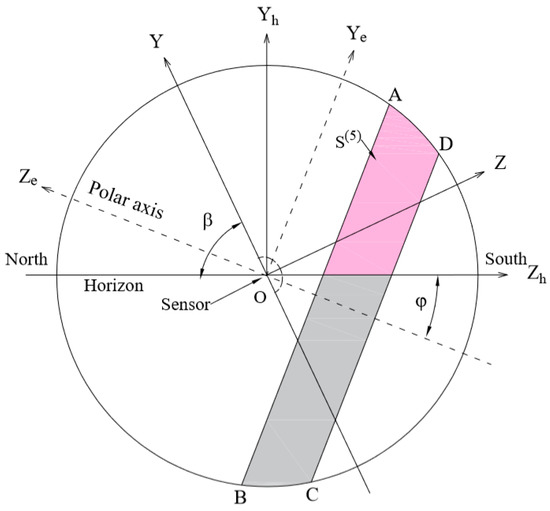
Figure 15. Schematic diagram for the calculation of $S_e$ while ${\varphi }_{e,l}\ge \pi /2$.

${\left[{\varphi }_{e,l},\left(\pi -\phi \right)\right]}_{min}$ is the minimum of ${\varphi }_{e,l}$. and $\left(\pi -\phi \right)$, ${\left[{\varphi }_{e,r},\left(\pi -\phi \right)\right]}_{min}$ is the minimum of ${\varphi }_{e,r}$ and $\left(\pi -\phi \right)$.

(2) While ${\varphi }_{e,l}<\pi /2<{\varphi }_{e,r}$ and $\beta \ge {\varphi }_{e,l}+\phi$, shown as Figure 16, $S^{\left(6\right)}$ is the area that is projected on the plane of $Y_{e}O{Z}_e$ by the spherical area shaded by the shadow band and is between the axis of $Y$ and $Y_e$, and will be used to represent the area in the following discussions,. Then, the Equation (43) will be written as

$$S_e={{\displaystyle \int }}_{{\alpha }_{e,w,1}}^{{\alpha }_{e,w,2}}{{\displaystyle \int }}_{\frac{\pi }{2}}^{{\varphi }_{e,r}}{ℱ}_{e}d\varphi d\alpha +{{\displaystyle \int }}_{{\alpha }_{e,i,1}}^{{\alpha }_{e,i,2}}{{\displaystyle \int }}_{{\left[{\varphi }_{e,l},\left(\beta -\phi \right)\right]}_{max}}^{\frac{\pi }{2}}{ℱ}_{e}d\varphi d\alpha$$

(52)

in which

$${\alpha }_{e,i,1}={\sin }^{-1}\left[-\tan \left(\phi -\beta \right)\cot \left(\varphi \right)\right]$$

(53)

$${\alpha }_{e,i,2}=\pi -{\alpha }_{e,i,1}$$

(54)

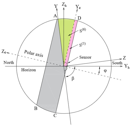
Figure 16. Schematic diagram for the calculation of $S_e$ while ${\varphi }_{e,l}<\pi /2<{\varphi }_{e,r}$ and $\beta >{\varphi }_{e,l}+\phi$.

${\left[{\varphi }_{e,l},\left(\beta -\phi \right)\right]}_{max}$ is the maximum of ${\varphi }_{e,l}$ and $\left(\beta -\phi \right)$.

(3) While ${\varphi }_{e,l}<\pi /2<{\varphi }_{e,r}$ and $\beta <{\varphi }_{e,l}+\phi$ and shown as Figure 17, $S^{\left(7\right)}$ is the area that is projected on the plane of $Y_{e}O{Z}_e$ by the spherical area shaded by the shadow band and is between the axis of $Y$ and $Y_e$, and this will be used to represent the area in the following discussions. However, $S^{\left(7\right)}$ is different from $S^{\left(6\right)}$, which can be found in Figure 17. Therefore, the Equation (43) is written as

$${\mathrm{S}}_e={{\displaystyle \int }}_{{\alpha }_{e,w,1}}^{{\alpha }_{e,w,2}}{{\displaystyle \int }}_{\frac{\pi }{2}}^{{\left[{\varphi }_{e,r},\left(\phi -\beta \right)\right]}_{min}}{ℱ}_{e}d\varphi d\alpha +{{\displaystyle \int }}_{{\alpha }_{e,i,1}}^{{\alpha }_{e,i,2}}{{\displaystyle \int }}_{{\left[{\varphi }_{e,l},\left(\phi -\beta \right)\right]}_{max}}^{\frac{\pi }{2}}{ℱ}_{e}d\varphi d\alpha$$

$$+{{\displaystyle \int }}_0^{2\pi }{{\displaystyle \int }}_{{\left[{\varphi }_{e,l},\left(\phi -\beta \right)\right]}_{min}}^{\phi -\beta }{ℱ}_{e}d\varphi d\alpha$$

(55)

in which ${\left[{\varphi }_{e,r},\left(\phi -\beta \right)\right]}_{min}$, ${\left[{\varphi }_{e,l},\left(\phi -\beta \right)\right]}_{max}$ and ${\left[{\varphi }_{e,l},\left(\phi -\beta \right)\right]}_{min}$ are the minimum of ${\varphi }_{e,r}$ and $\left(\phi -\beta \right)$, and the maximum and the minimum of ${\varphi }_{e,l}$ and $\left(\phi -\beta \right)$, respectively.

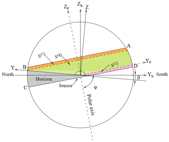
Figure 17. Schematic diagram for the calculation of $S_e$ while ${\varphi }_{e,l}<\pi /2<{\varphi }_{e,r}$ and $\beta \le {\varphi }_{e,l}+\phi$.

If the axis $Y$ is between the points A and B, it should be mentioned that the third term of Equation (55) on the right-hand side is equal to zero and $S^{\left(7\right)}$ will not exist anymore.

(4) While ${\varphi }_{e,r}\le \pi /2$ and $\beta \ge {\varphi }_{e,l}+\phi$, shown as Figure 18, the Equation (43) is written as

$$S_e={{\displaystyle \int }}_{{\alpha }_{e,i,1}}^{{\alpha }_{e,i,2}}{{\displaystyle \int }}_{{\left[{\varphi }_{e,l},\left(\beta -\phi \right)\right]}_{max}}^{{\left[{\varphi }_{e,r},\left(\beta -\phi \right)\right]}_{max}}{ℱ}_{e}d\varphi d\alpha$$

(56)

in which ${\left[{\varphi }_{e,r},\left(\beta -\phi \right)\right]}_{max}$ is the maximum of ${\varphi }_{e,r}$ and $\left(\beta -\phi \right)$.

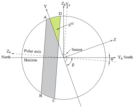
Figure 18. Schematic diagram for the calculation of $S_e$ while ${\varphi }_{e,r}\le \pi /2$ and $\beta >{\varphi }_{e,l}+\phi$.

(5) While ${\varphi }_{e,r}\le \pi /2$ and $\beta <{\varphi }_{e,l}+\phi$, shown as Figure 19, the Equation (43) will become

$${\mathrm{S}}_e={{\displaystyle \int }}_{{\alpha }_{e,i,1}}^{{\alpha }_{e,i,2}}{{\displaystyle \int }}_{{\left[{\varphi }_{e,l},\left(\phi -\beta \right)\right]}_{max}}^{{\left[{\varphi }_{e,r},\left(\phi -\beta \right)\right]}_{max}}{ℱ}_{e}d\varphi d\alpha +{{\displaystyle \int }}_0^{2\pi }{{\displaystyle \int }}_{{\left[{\varphi }_{e,l},\left(\phi -\beta \right)\right]}_{min}}^{{\left[{\varphi }_{e,r},\left(\phi -\beta \right)\right]}_{min}} {ℱ}_{e}d\varphi d\alpha$$

(57)

in which ${\left[{\varphi }_{e,r},\phi -\beta \right]}_{max}$ is the maximum of ${\varphi }_{e,r}$ and $\left(\phi -\beta \right)$.

Figure 19. Schematic diagram for the calculation of $S_e$ while ${\varphi }_{e,r}\le \pi /2$ and $\beta \le {\varphi }_{e,l}+\phi$.

If the axis $Y$ is between the points A and B, the second term of Equation (57) on the right-hand side is equal to zero and $S^{\left(7\right)}$ will not exist.

2.2.2. Calculation of $H_e$

The area $H_{e,s}$ projected from the sky sphere onto the radiation sensor in equatorial coordinates can be calculated by two different expressions according to the correlation of $\beta$ and $\phi$.

(1) While $\beta \ge \phi$, the expression of $H_e$ is

$$H_{e,s}={{\displaystyle \int }}_{{\alpha }_{e,i,1}}^{{\alpha }_{e,i,2}}{{\displaystyle \int }}_{\beta -\phi }^{\frac{\pi }{2}}{ℱ}_{e}d\varphi d\alpha +{{\displaystyle \int }}_{{\alpha }_{e,w,1}}^{{\alpha }_{e,w,2}}{{\displaystyle \int }}_{\frac{\pi }{2}}^{\pi -\phi }{ℱ}_{e}d\varphi d\alpha$$

(58)

(2) While $\beta <\phi$, the expression of $H_e$ is

$$H_{e,s}={{\displaystyle \int }}_0^{2\pi }{{\displaystyle \int }}_0^{\phi -\beta } {ℱ}_{e}d\varphi d\alpha +{{\displaystyle \int }}_{{\alpha }_{e,i,1}}^{{\alpha }_{e,i,2}}{{\displaystyle \int }}_{\phi -\beta }^{\frac{\pi }{2}}{ℱ}_{e}d\varphi d\alpha +{{\displaystyle \int }}_{{\alpha }_{e,w,1}}^{{\alpha }_{e,w,2}}{{\displaystyle \int }}_{\frac{\pi }{2}}^{\pi -\phi }{ℱ}_{e}d\varphi d\alpha$$

(59)

$H_{e,g}$ has the same expression as $H_{h,g}$. The area $H_e$ in Equation (41) is calculated by

$$H_e=H_{e,s}+H_{e,g}$$

(60)

3. Results and Discussions

To check whether the correction factor expressions obtained in the horizon and equatorial coordinates are correct or not, $C_h$ and $C_e$ were calculated and compared with each other, in which the latitude $\phi$ and day of the year varied from $0°$ to $90°$ and from 1 to 365, respectively. It is proved that $C_h$ is equal to $C_e$ under the same conditions even though their expressions of (2) and (41) are completely different. Some of the calculation results are listed in Table 1. $C_{h\&e}$ will be used to represent $C_h$ and $C_e$ in the following discussions.

Table 1. Comparisons of $C_h$, $C_e$, $C_{h\&e}$, $C_D$, ${\eta }_D$ while $\beta =0$.

$\mathit{\phi }(°)$	Day of the Year	${\mathit{C}}_{\mathit{h}\&\mathit{e}}(-)$		${\mathit{C}}_{\mathit{D}}(-)$	${\mathit{\eta }}_{\mathit{D}}(\%)$
		${\mathit{C}}_{\mathit{h}}(-)$	${\mathit{C}}_{\mathit{e}}(-)$
0	81	1.2552	1.2552	1.2604	0.45
	350	1.172	1.172	1.1722	0.02
25	81	1.2262	1.2262	1.2308	0.38
	350	1.1047	1.1047	1.1034	0.12
50	81	1.1514	1.1514	1.1534	0.17
	350	1.0341	1.0341	1.0318	0.22
89	81	1.0266	1.0266	1.0036	2.23
	350	1.0	1.0	*	*

* The data cannot be calculated by the expressions in references.

3.1. Comparisons with the Results Calculated by Drummond’s Expression

The width and the radius of the shadow ring are supposed to be 65 mm and 200 mm, respectively, for the discussions in this section. While comparing the corrector factor $C_{h\&e}$ with the results calculated by the expression of Drummond [6] at $\beta =0$, the relative deviation ${\eta }_D$ is introduced by

$${\eta }_D=\frac{\left|C_D-C_{h\&e}\right|}{C_{h\&e}}\times 100\%$$

(61)

To investigate the variations of $C_{h\&e}$, $C_D$, ${\eta }_D$ at different latitudes and days of the year, the latitudes $0°$, $25°$, $50°$, $89°$ in the northern hemisphere and the day numbers 81 and 350 of the year were chosen to do the calculations firstly. The results are shown in Table 1. It can be seen in Table 1 that $C_{h\&e}$ is equal to 1.0 but $C_D$ cannot be calculated at day number 350 and at latitude $89°$ in northern hemisphere. Secondly, $C_{h\&e}$, $C_D$, and ${\eta }_D$ were calculated for the latitudes varying from $0°$ to $90°$ in the northern hemisphere and for days of the year varying from 1 to 365. The results are shown in Figure 20, Figure 21 and Figure 22.

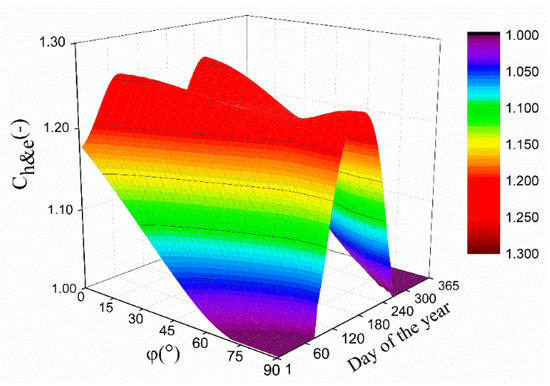
Figure 20. Surface chart of $C_{h\&e}$ varying with day of the year and different latitudes at $\beta =0$.

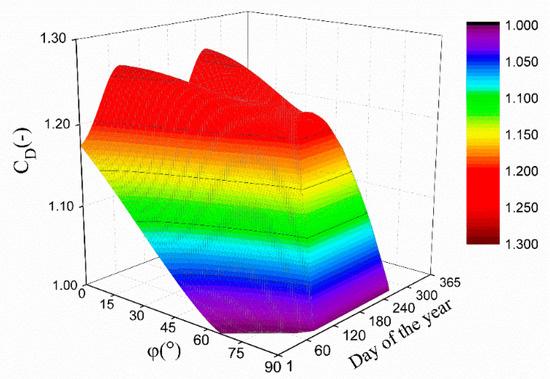
Figure 21. Surface chart of $C_D$ varying with day of the year and different latitudes at $\beta =0$.

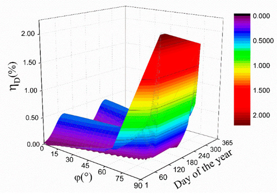
Figure 22. Surface chart of ${\eta }_D$ varying with day of the year and different latitudes at $\beta =0$.

While the latitudes are in the Artic Circle, it can be found that the $C_{h\&e}$ is equal to 1.0 at some days in Table 1 and in Figure 20 when polar nights happen, however, $C_D$ and ${\eta }_D$ cannot be calculated in some days and the points in Table 1; in Figure 21 and Figure 22 it is missing due to a reason that will be discussed in Section 3.3. For those $C_D$ which can be calculated by the expression of Drummond [6], the maximum of the relative deviations ${\eta }_D$ is 2.23% in Figure 22 while the latitude $\phi$ and day of the year are $89°$ and 81 respectively. It can be understood that our expressions for and $C_e$ are indirectly validated by the experimental data in Drummond’s paper [6], from the comparison of our results with the expressions of Drummond.

3.2. Comparisons with the Experimental Data and the Results Calculated by Bureck’s Expression

The width and the radius of the shadow ring are 50 mm and 200 mm, respectively for the discussions in this section. The factors $C_{h\&e}$ calculated by our expressions will be compared with the experimental results and $C_B$ in Burek’s paper [7]. It is shown in Table 2.

Table 2. Experimental results and comparison with calculated values of $C_B$.

Date of Experiment	Solarimeter $\mathbf{Tilt} \mathit{\beta }$ (Degrees)	Measured Correction		Calculated Correction
		All Day	$\mathbf{Noon}\pm$ 1 h	$\mathit{\rho }=0.26$		$\mathit{\rho }=0.5$		$\mathit{\rho }=0.8$		$\mathit{\rho }=1.0$
				${\mathit{C}}_{\mathit{h}\&\mathit{e}}$	${\mathit{C}}_{\mathit{B}}$	${\mathit{C}}_{\mathit{h}\&\mathit{e}}$	${\mathit{C}}_{\mathit{B}}$	${\mathit{C}}_{\mathit{h}\&\mathit{e}}$	${\mathit{C}}_{\mathit{B}}$	${\mathit{C}}_{\mathit{h}\&\mathit{e}}$	${\mathit{C}}_{\mathit{B}}$
20 August–4 September	41	1.18	1.18	1.20	1.22	1.20	1.21	1.19	1.19	1.18	1.18
4 September–18 September	48	1.22	1.20	1.22	1.25	1.21	1.22	1.19	1.20	1.19	1.19
21 September–30 September	52	1.25	1.23	1.22	1.26	1.21	1.23	1.19	1.20	1.19	1.19
4 October–14 October	58	1.20	1.20	1.22	1.27	1.21	1.24	1.19	1.20	1.18	1.19

As shown in Table 2, both the correction factors calculated by our expressions and by Bureck’s expression [7] are in agreement with the experimental results. In order to comprehensively understand the difference between the correction factors calculated by our expressions and by Bureck’s expression [7] at the different latitudes $\phi$, slope angle $\beta$ and day of the year, the relative deviation ${\eta }_B$ is introduced and expressed as

$${\eta }_B=\frac{\left|C_B-C_{h\&e}\right|}{C_{h\&e}}\times 100\%$$

(62)

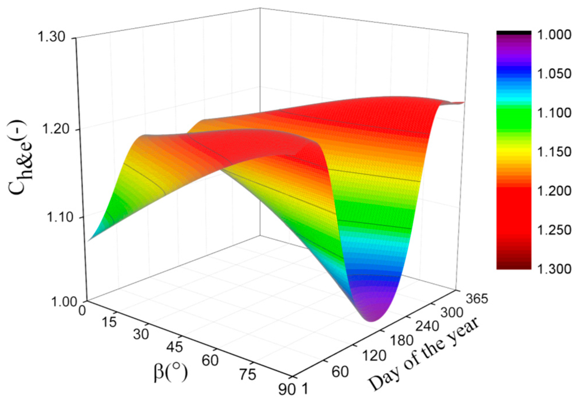
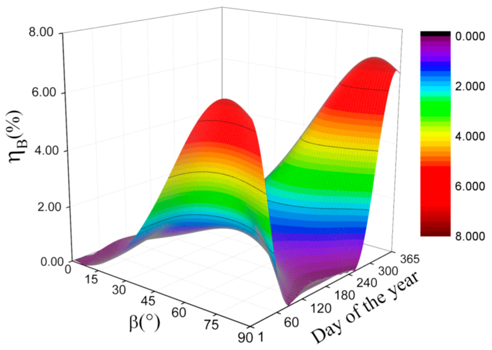
Supposing that the latitude $\phi$ in northern hemisphere is $30°$ and ground reflectance $\rho$ is 0.2, slope angle $\beta$ changes from $1°$ to $90°$ and day number of the year varies from 1 to 365, the variations of $C_{h\&e}$, $C_B$, ${\eta }_B$ with different slope angles and days of the year are shown in Figure 23, Figure 24 and Figure 25.

Figure 23. Surface chart of $C_{h\&e}$ varying with $\beta$ and day of the year at $30° \mathrm{N}$ and $\rho =0.2$.

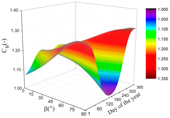
Figure 24. Surface chart of $C_B$ varying with $\beta$ and day of the year at $30° \mathrm{N}$ and $\rho =0.2$.

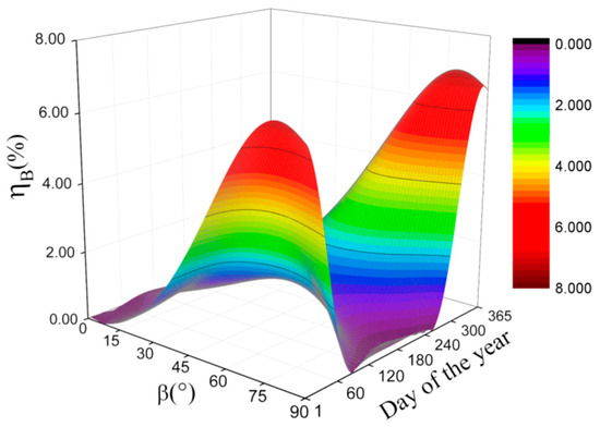
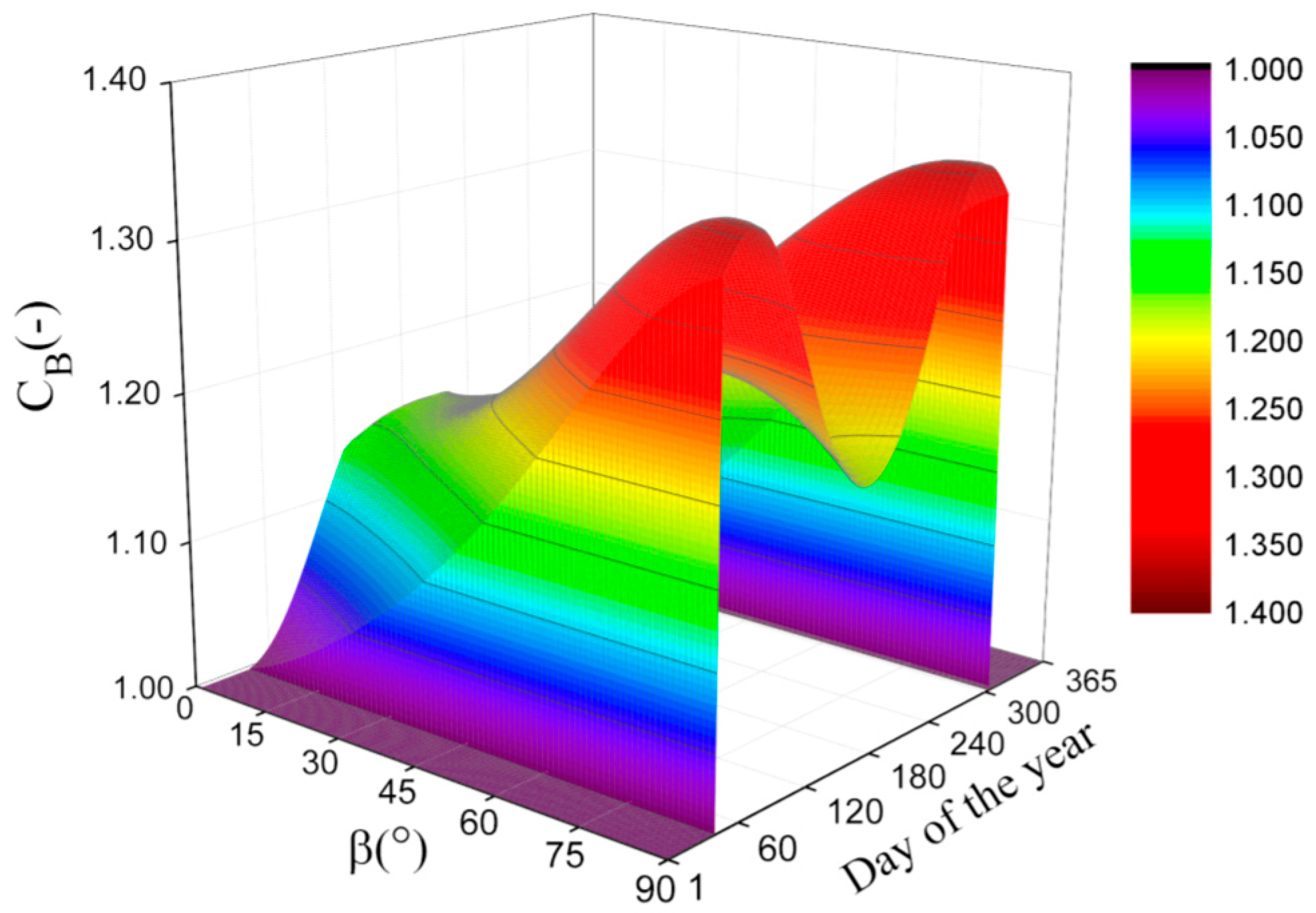
Figure 25. Surface chart of ${\eta }_B$ varying with $\beta$ and day of the year at $30° \mathrm{N}$ and $\rho =0.2$.

As shown in Figure 23 and Figure 24, the variational curves of $C_{h\&e}$ and $C_B$ with day of the year have two maxima while $\beta$ is fixed. It is shown in Figure 25 that the peaks of the relative deviations ${\eta }_B$ between precise $C_{h\&e}$ and $C_B$ appear in the ranges of bigger $\beta$ and the first or the final days of the year. It was found that the two maxima of ${\eta }_B$ are 6.88% and 6.98%, while $\beta$ is $80°$ and the days of the year are 1 and 355, respectively. The peaks of the surface charts of Figure 23 and Figure 24 also appear in the ranges of a larger $\beta$ and the first or the final days of the year.

Supposing that the latitude $\phi$ in northern hemisphere is 75$°$ and ground reflectance $\rho$ is 0.2, slope angle $\beta$ changes from $1°$ to $90°$ and day number of the year varies from 1 to 365, the variations of $C_{h\&e}$, $C_B$, ${\eta }_B$ with different slope angles and days of the year were investigated and shown in Figure 26, Figure 27 and Figure 28.

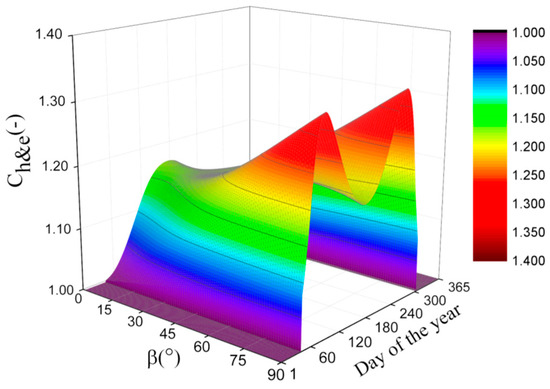
Figure 26. Surface chart of $C_{h\&e}$ varying with $\beta$ and day of the year at $75° \mathrm{N}$ and $\rho =0.2$.

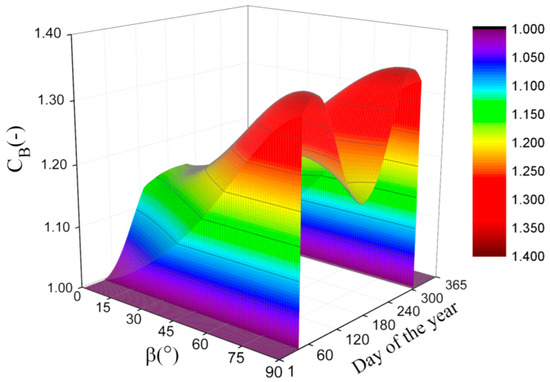
Figure 27. Surface chart of $C_B$ varying with $\beta$ and day of the year at $75° \mathrm{N}$ and $\rho =0.2$.

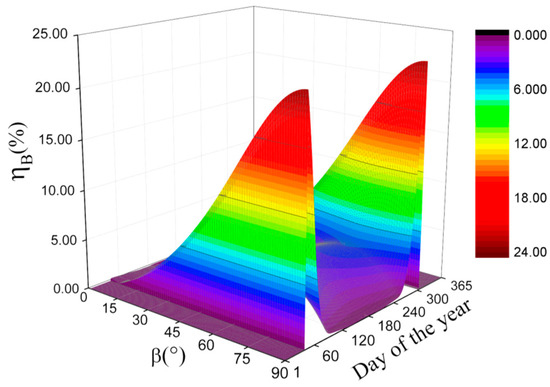
Figure 28. Surface chart of ${\eta }_B$ varying with $\beta$ and day of the year at $75° \mathrm{N}$ and $\rho =0.2$.

As shown as in Figure 26 and Figure 27, the correction factors are equal to 1.0 both for $C_{h\&e}$ and $C_B$ during the period of the polar nights. In non-polar night situations, the peaks of the surface charts of $C_{h\&e}$, $C_B$, and ${\eta }_B$ appear in the ranges of a larger $\beta$ and the first or the final days of the year, which are shown in Figure 26, Figure 27 and Figure 28. As shown in Figure 28, the two maxima of ${\eta }_B$ are 22.97% and 22.70% while $\beta$ is $90°$ and the days of the year are 41 and 303 respectively, but it must be mentioned that $C_B$ and ${\eta }_B$ cannot be calculated in some days and the points in Figure 27 and Figure 28 are missing due to a reason that will be discussed in Section 3.3.

3.3. Discussions on $C_D$, $C_B$, $C_h$ and $C_e$

It must be pointed out that the sunrise solar hour angle $\omega$ must be known to calculate the correction factors $C_D$ and $C_B$ by the expressions of Drummond [6] and Burek et al. [7]. While the slope angle is $\beta$ and a tilted surface is oriented towards the equator, the sunrise solar hour angle $\omega$ for a tilted surface is given by

$$\cos \left(\omega \right)=-\tan \left(\phi -\beta \right)\tan \left(\delta \right)$$

(63)

While $\left|-\tan \left(\phi -\beta \right)\tan \left(\delta \right)\right|>1$, the sunrise solar hour angle $\omega$ cannot be calculated by the Equation (63). Therefore, the correction factors $C_D$ and $C_B$ could not be calculated too. However, the correction factors $C_h$ and $C_e$ can be calculated by our expressions in that situation. Therefore, some points in Figure 21 and Figure 27 are missing in some cases such as the latitudes being in the Artic Circle. The surface charts in Figure 21 and Figure 27 are not smooth and not continual, but the surface charts in Figure 20 and Figure 26 are smooth and continual even if the latitudes are in Artic Circle, because the correction factors $C_h$ and $C_e$ can be calculated in ranges of $0\le \beta \le 90°$, $-90°\le \phi \le 90°$ and for any day of the year. There is not any restriction for the calculations of $C_h$ and $C_e$ because the sunrise solar hour angle $\omega$ doesn’t appear in our expressions.

On the other hand, the expressions of Drummond [6] and Burek et al. [7] for the correction factors $C_D$ and $C_B$ were obtained on the basis of two assumptions which are mentioned in Section 1. Their calculation results are approximate. However, our expressions for the correction factors $C_h$ and $C_e$ are achieved by mathematical analysis without any assumptions. The results are precise. Due to the maximum difference between the results calculated by our expressions and Drummond’s expression [6] being less than 2.3% (see Figure 22) when the width and radius of the shadow band are 50 mm and 200 mm, respectively, this means that the influence of the assumptions for Drummond’s expression on the calculation results is negligible under the conditions. However, the maximum relative deviation between the results calculated by our expressions and Burek’s expression [7] is more than 22%, while $\phi =75°$ and $\rho =0.2$ (see Figure 28). It means that the influence of the assumptions for Burek’s expression in some cases on the calculation results is significant.

3.4. Discussions on ${\eta }_D$ and ${\eta }_B$

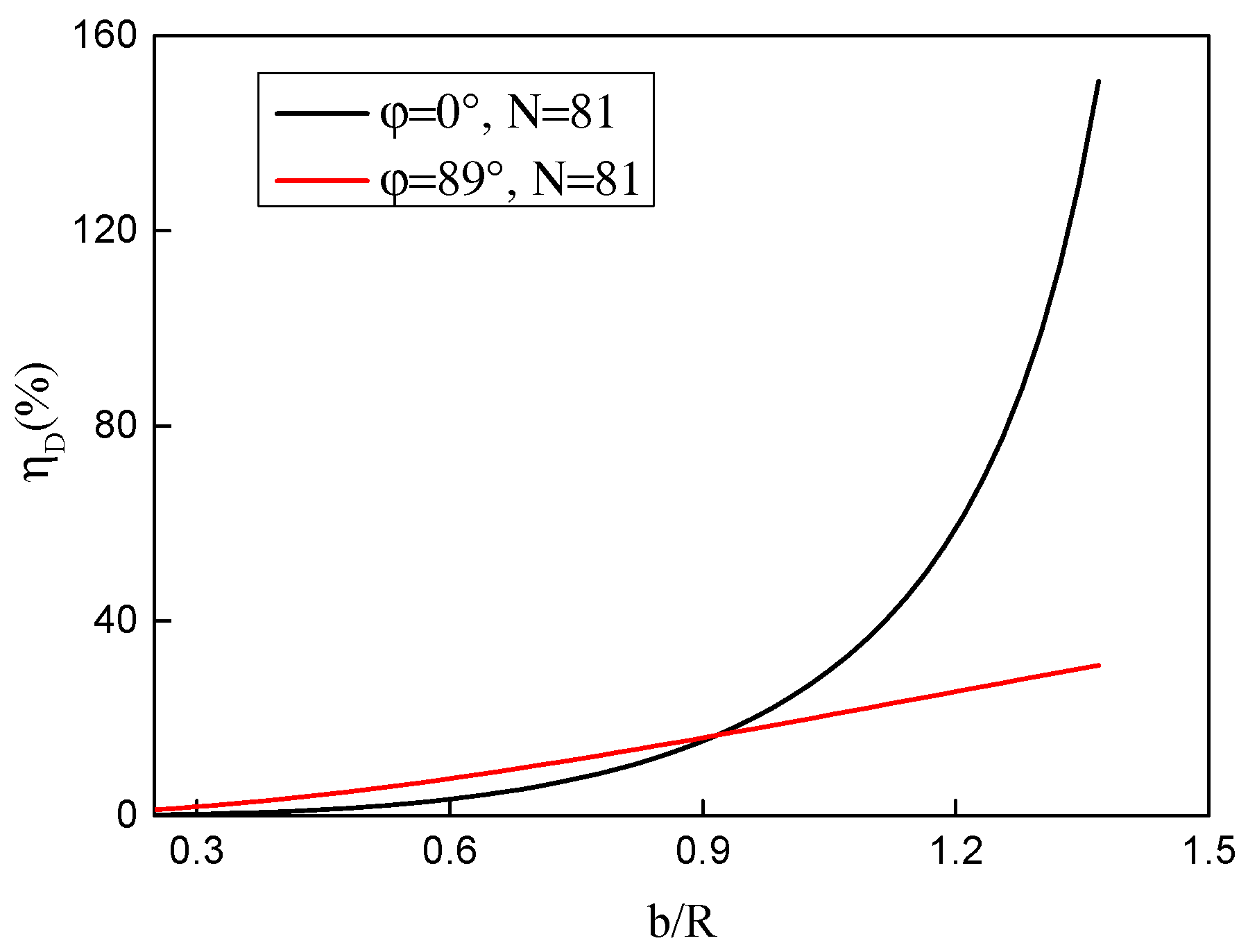
The ratios of width and radius of the shadow band were 0.325 and 0.25, as discussed in Section 3.1 and Section 3.2, respectively. On the basis of the ratio 0.325, the maximum value of ${\eta }_D$ for all possibly calculated values is less than 2.3%. It means that the deviation between the results calculated by our expressions and Drummond’s expression [6] is small. However, it was found that the accuracies of the results calculated by Drummond’s expression are related to the ratios. It is easily to think that the relative deviation ${\eta }_D$ between $C_{h\&e}$ and $C_D$ should also be related to the ratios if $C_{h\&e}$ is a precise value. As shown in Figure 29, they are the correlation curves of ${\eta }_D$ with the ratios at the two locations, for which their latitudes are $0°$ and $89°$, for the 81st day of the year. It can be seen from the curves in Figure 29 that the relative deviation ${\eta }_D$ will become very small when the ratio of width and radius of the shadow band is very small. But the relative deviation ${\eta }_D$ increases with the increase of the ratio. The deviation between $C_{h\&e}$ and $C_D$ will become larger with the increase of the ratio.

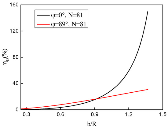
Figure 29. Correlation curves of ${\eta }_D$ with the ratios of width and radius of the shadow band.

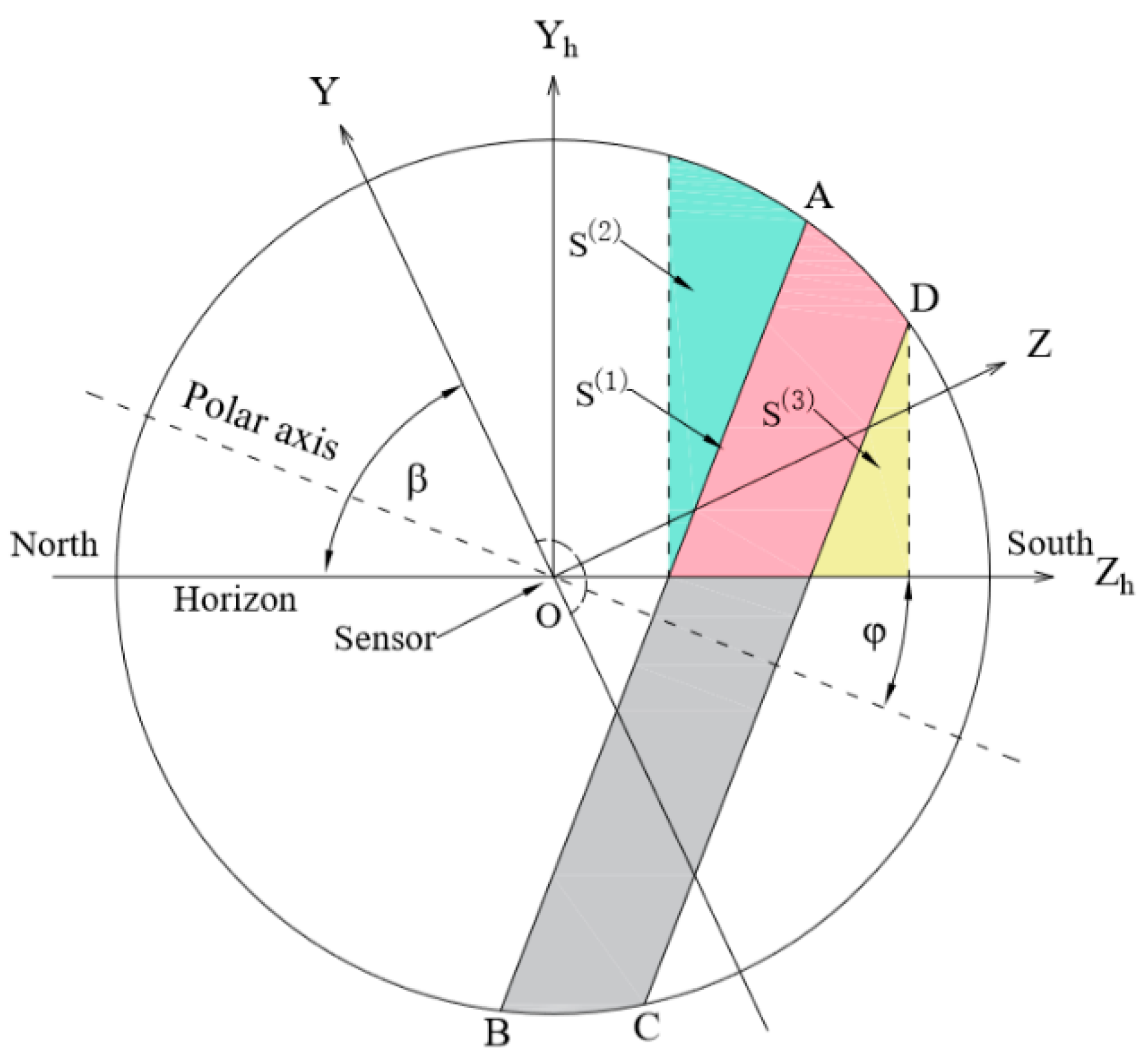
After carefully investigating the discussions on our expressions and on Burek’s expression [7], there are two main reasons as to why the maximum value of ${\eta }_B$ can be up to 22.97% in Figure 28 and why there exists a big deviation between the results calculated by our expressions and by Burek’s expression.

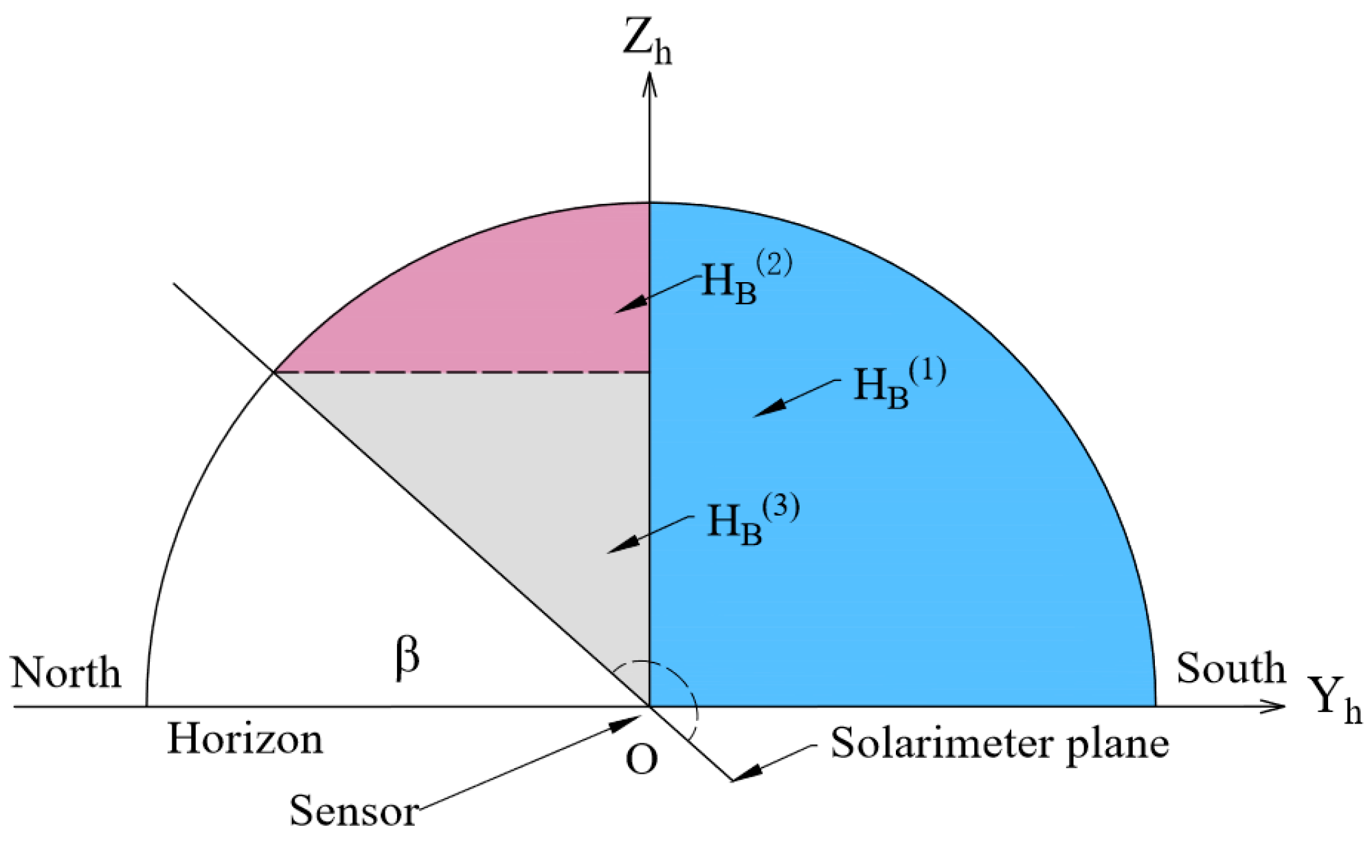
The first reason is that a part of the spherical area was not considered during the calculation of Equation (2) for $h_s$ in Burek’s paper [7]. As shown in Figure 30, $H_B^{\left(1\right)}$, $H_B^{\left(2\right)}$ and $H_B^{\left(3\right)}$ are the areas projected on the plane of $Y_{h}O{Z}_h$ by three parts of spherical areas. The spherical areas connected with $H_B^{\left(1\right)}$ and $H_B^{\left(2\right)}$ are considered during the calculation of Equation (2) for $h_s$ in Burek’s paper, but the spherical area connected with $H_B^{\left(3\right)}$ is not taken into account. The spherical area connected with $H_B^{\left(2\right)}$ is considered during the calculation of Equation (1) for $h_{seg}$ in Burek’s paper [7].

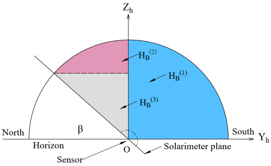
Figure 30. Schematic diagram for the calculation of $h_s$ in Burek’s paper [7].

The second reason is that Equation (6) in Burek’s paper [7] for $S_B$ is approximate. When the latitude and the slope angle are high and solar elevation angle is low at noon, the accuracy of the $S_B$ calculated by Equation (6) in Burek’s paper will become worse. For easily understanding the differences between $S_{h\&e}$ and $S_B$ as well as between $H_{h\&e}$ and $H_B$, some calculated results are shown in Table 3. During the calculations in Table 3, the ground reflectance $\rho$ and the width and radius of the shadow band are considered to be 0.2, 50 mm and 200 mm respectively.

Table 3. Calculated values and comparisons of S, H, C.

$\mathit{\phi }(°)$	$\mathbf{Slope} \mathbf{Angle} (°)$	Day of the Year	${\mathit{S}}_{\mathit{h}\&\mathit{e}}$ ${\left(\mathbf{c}\mathbf{m}\right)}^2$	${\mathit{S}}_{\mathit{B}}$ ${\left(\mathbf{c}\mathbf{m}\right)}^2$	${\mathit{H}}_{\mathit{h}\&\mathit{e}}$ ${\left(\mathbf{c}\mathbf{m}\right)}^2$	${\mathit{H}}_{\mathit{B}}$ ${\left(\mathbf{c}\mathbf{m}\right)}^2$	${\mathit{C}}_{\mathit{h}\&\mathit{e}}$	${\mathit{C}}_{\mathit{B}}$	${\mathit{\eta }}_{\mathit{B}}$ (%)
75	60	41	55.17	160.66	1076.49	941.93	1.054	1.2056	14.39
		303	56.99	161.11	1074.94	940.57	1.056	1.2067	14.27
	90	41	61.80	201.08	807.37	807.37	1.0829	1.3316	22.97
		303	63.78	201.13	806.20	806.20	1.0859	1.3324	22.70

As shown in Table 3, the relative deviation ${\eta }_B$ is influenced only by the second reason and the first reason is not existent when the slope angle $\beta$ is equal to $90°$, which can be understood by Figure 30. In that situation, the areas $H_{h\&e}$ are the same as $H_B$ at any day of the year but the area $S_{h\&e}$ is not the same as $S_B$. When the slope angle $\beta$ is not equal to $90°$, the relative deviation ${\eta }_B$ is influenced by both the first reason and the second reason. It means that both areas $H_{h\&e}$ and $S_{h\&e}$ are not equal to $H_B$ and $S_B$ at the same day, respectively. However, if all three parts of the spherical area related to the projected areas $H_B^{\left(1\right)}$, $H_B^{\left(2\right)}$ and $H_B^{\left(3\right)}$ in Figure 30 are considered during the calculation of Equation (2) for $h_s$ in Burek’s paper [7], the area $H_B$ should be the same as $H_{h\&e}$ at the same day, latitude and slope angle.

4. Conclusions

In this paper the shadow band correction factors $C_h$ and $C_e$ were theoretically investigated, and the expressions in horizon and equatorial coordinates under isotropic conditions are given. The calculation results of $C_h$ and $C_e$ were compared with the results of $C_D$ and $C_B$ by Drummond [6] and by Burek et al. [7] respectively. It can be concluded that

• $C_h$ and $C_e$ can be calculated by the expressions in any case ($0°\le \beta \le 90°,-90°\le \phi \le 90°$), and the results calculated by the different expressions in horizon and equatorial coordinates are equal each other under the same conditions. The correction factors calculated by our expressions are in good agreement with the experimental results from Burek’s paper [7]. Additionally, our expressions are indirectly validated by the experimental results from Drummond’s paper [6] because the maximum relative deviation ${\eta }_D$ is less than 2.3%. It is proven that the expressions of $C_h$ and $C_e$ are correct and can give the precise correction factors under isotropic conditions.
• While $\beta =0$ and the ratio of width and radius of the shadow band is small under isotropic weather conditions, it is suggested to use the expression of Drummond [6] for the correction factors if it is possible, because the calculation by Drummond’s expression is easier. However, our expressions must be used for the correction factors $C_h$ and $C_e$ when the ratio of the width and radius of the shadow band is large or while the latitude $\phi$ and the declination $\delta$ are satisfied with the condition of $\left|-\tan \left(\phi \right)\tan \left(\delta \right)\right|>1$, because the expression of Drummond cannot be used to calculate the correction factor $C_D$ under those conditions.
• While $\beta >0$ under isotropic weather conditions, it is suggested to use our expressions for the correction factors. Especially, while the latitude $\phi$ and the declination $\delta$ are satisfied with the condition of $\left|-\tan \left(\phi -\beta \right)\tan \left(\delta \right)\right|>1$, our expressions must be used for the correction factors because the expression of Burek [7] cannot be used to calculate the correction factor $C_B$ under those conditions. Additionally, while the latitude $\phi$ is close to or in the polar circle, the influences of the assumptions for Burek’s expression in some cases on the calculation results are significant. As an instance, the maximum relative deviation between the results calculated by our expressions and Burek’s expression [7] is more than 22%, while $\phi =75°$ and $\rho =0.2$.

References

- de Oliveira, A.P.; Machado, A.J.; Escobedo, J.F. A New Shadow-Ring Device for Measuring Diffuse Solar Radiation at the Surface. J. Atmos. Ocean. Technol. 2002, 19, 698–708. [Google Scholar] [CrossRef]
- Robinson, N.; Stoch, L. Sky radiation measurement and corrections. J. Appl. Meteorol. Climatol. 1964, 3, 179–181. [Google Scholar] [CrossRef]
- Brooks, M.J. Performance characteristics of a perforated shadow band under clear sky conditions. Sol. Energy 2010, 84, 2179–2194. [Google Scholar] [CrossRef]
- de Simón-Martín, M.; Alonso-Tristán, C.; González-Peña, D.; Díez-Mediavilla, M. New device for the simultaneous measurement of diffuse solar irradiance on several azimuth and tilting angles. Sol. Energy 2015, 119, 370–382. [Google Scholar] [CrossRef]
- Brooks, M.J.; Roberts, L.W. A data processing algorithm for the perforated shadow band incorporating a ray trace model of pyranometer exposure. In Reliability of Photovoltaic Cells, Modules, Components, and Systems III; SPIE: Bellingham, WA, USA, 2016; Volume 7773, pp. 77730W-1–77730W-9. [Google Scholar]
- Drummond, A.J. On the measurement of sky radiation. Arch. Meteor. Geophys. Bioklim 1956, 7, 413–436. [Google Scholar] [CrossRef]
- Burek, S.A.M.; Norton, B.; Probert, S.D. Analytical and experimental methods for shadow-band correction factors for solarimeters on inclined planes under isotropically diffuse and overcast skies. Sol. Energy 1988, 40, 151–160. [Google Scholar] [CrossRef]
- Rawlins, F.; Readings, C.J. The shade ring correction for measurements of diffuse irradiance under clear skies. Sol. Energy 1986, 37, 407–416. [Google Scholar] [CrossRef]
- Muneer, T.; Zhang, X. A new method for correcting shadow band diffuse irradiance data. ASME 2002, 124, 34–43. [Google Scholar] [CrossRef]
- Lebaron, B.A.; Michalsky, J.J.; Perez, R. A simple procedure for correcting shadow band data for all sky conditions. Sol. Energy 1990, 44, 249–256. [Google Scholar] [CrossRef]
- Kudish, A.I.; Ianetz, A. Analysis of diffuse radiation data for Beer Sheva: Measured (shadow ring) versus calculated (global horizontal beam) values. Sol. Energy 1993, 51, 493–503. [Google Scholar] [CrossRef]
- Batlles, F.J.; Olmo, F.J.; Alados-Arboledas, L. On shadow band correction methods for diffuse irradiance measurements. Sol. Energy 1995, 54, 105–114. [Google Scholar] [CrossRef]
- Vartiainen, E. An anisotropic shadow ring correction method for the horizontal diffuse irradiance measurements. Renew. Energy 1999, 17, 311–317. [Google Scholar] [CrossRef]
- Dal Pai, A.; Escobedo, J.F.; Dal Pai, E.; dos Santos, C.M. Estimation of hourly, daily and monthly mean diffuse radiation based on MEO shadow ring correction. Energy Procedia 2014, 57, 1150–1159. [Google Scholar] [CrossRef]
- Chaiyapinunt, S.; Ruttanasupa, P.; Ariyapoonpong, V.; Duanmeesook, K. A shadow-ring device for measuring diffuse solar radiation on a vertical surface in a tropical zone. Sol. Energy 2016, 136, 629–638. [Google Scholar] [CrossRef]
- Iqbal, M. An Introduction to Solar Radiation, 1st ed.; Academic Press, Inc.: New York, NY, USA, 1983; pp. 307–309. [Google Scholar]
Publisher’s Note: MDPI stays neutral with regard to jurisdictional claims in published maps and institutional affiliations. |
© 2022 by the authors. Licensee MDPI, Basel, Switzerland. This article is an open access article distributed under the terms and conditions of the Creative Commons Attribution (CC BY) license (https://creativecommons.org/licenses/by/4.0/).