
Framework for Energy-Averaged Emission Mitigation Technique Adopting Gasoline-Methanol Blend Replacement and Piston Design Exchange
 , ,
, ,
Abstract
:1. Introduction
2. Methods
3. Energy Conversion and Emission Measurement
4. Emission Formation Mechanism
5. Finite Element Analysis of Coated Piston Design Exchange
6. Response Surface Methodology
7. Results and Discussion
8. Evolution of Mathematical Model—Design of Experiment for Response Surface Methodology
8.1. Effect on Reaction Parameter
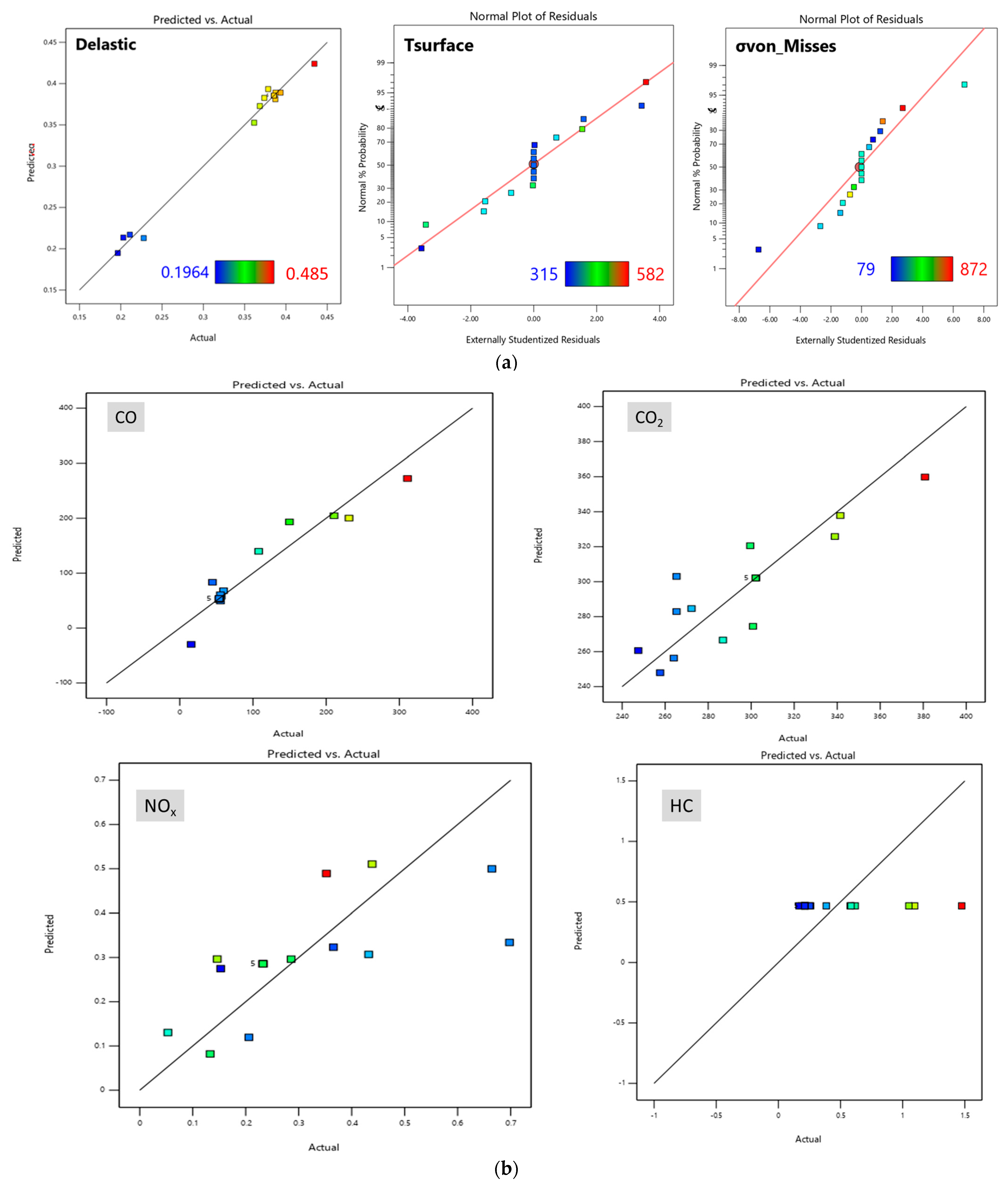
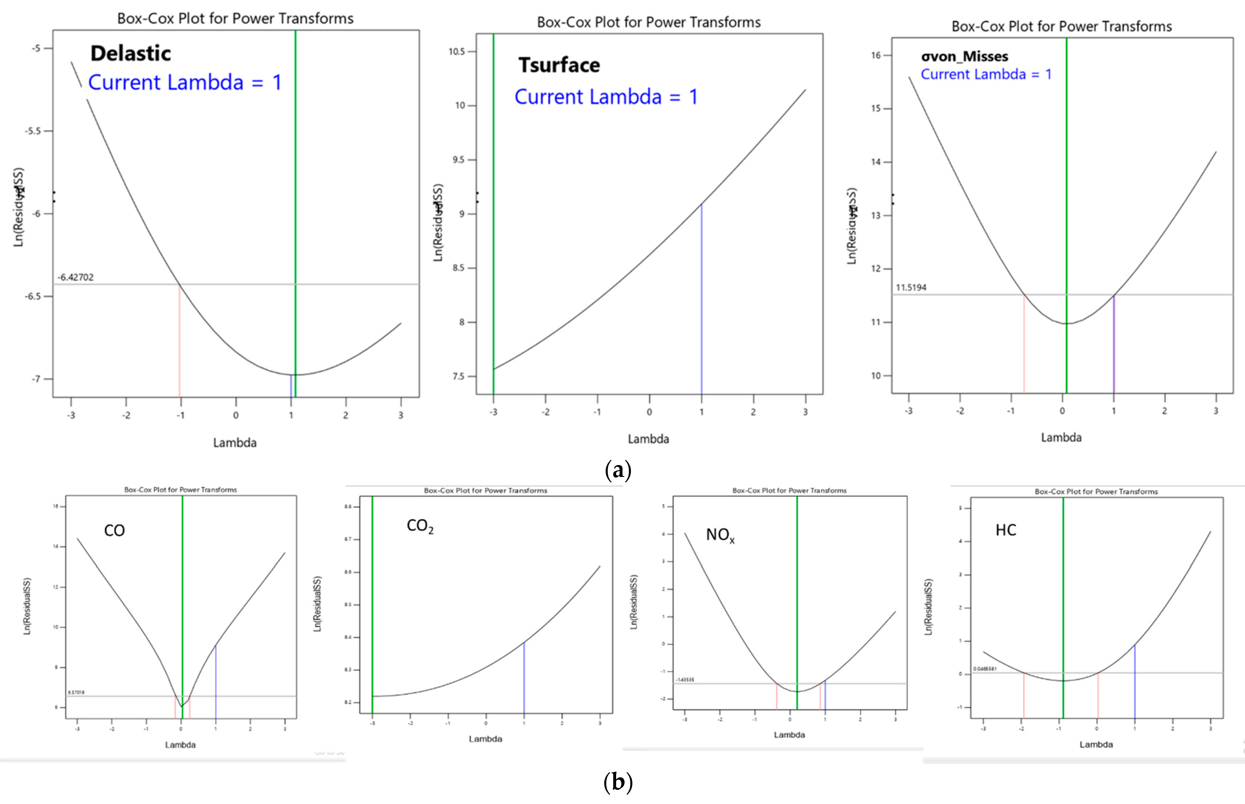
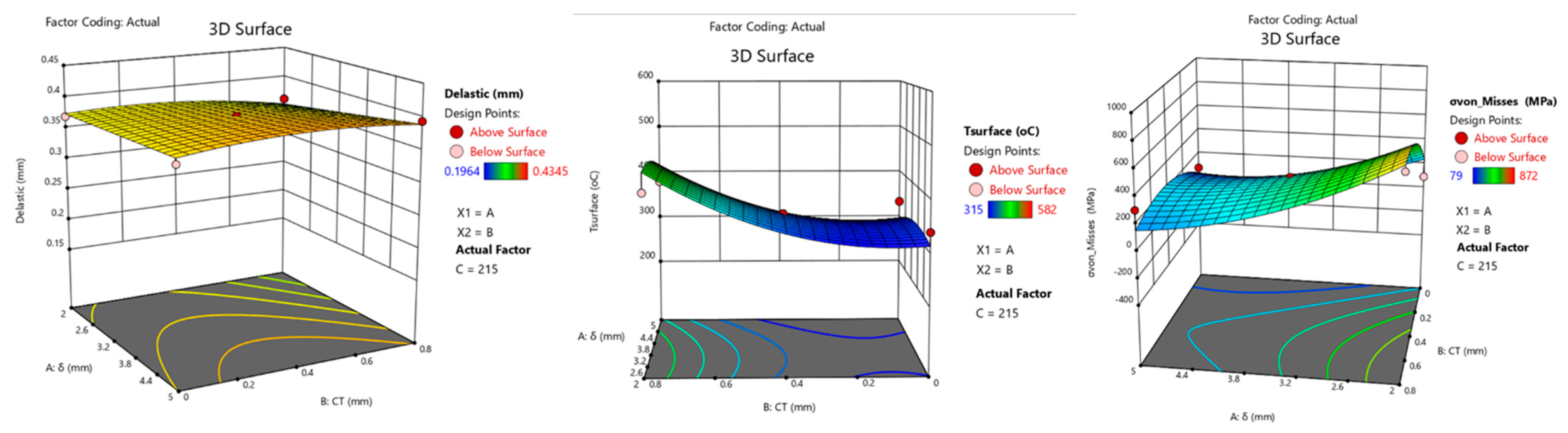
8.2. Effect on Delastic
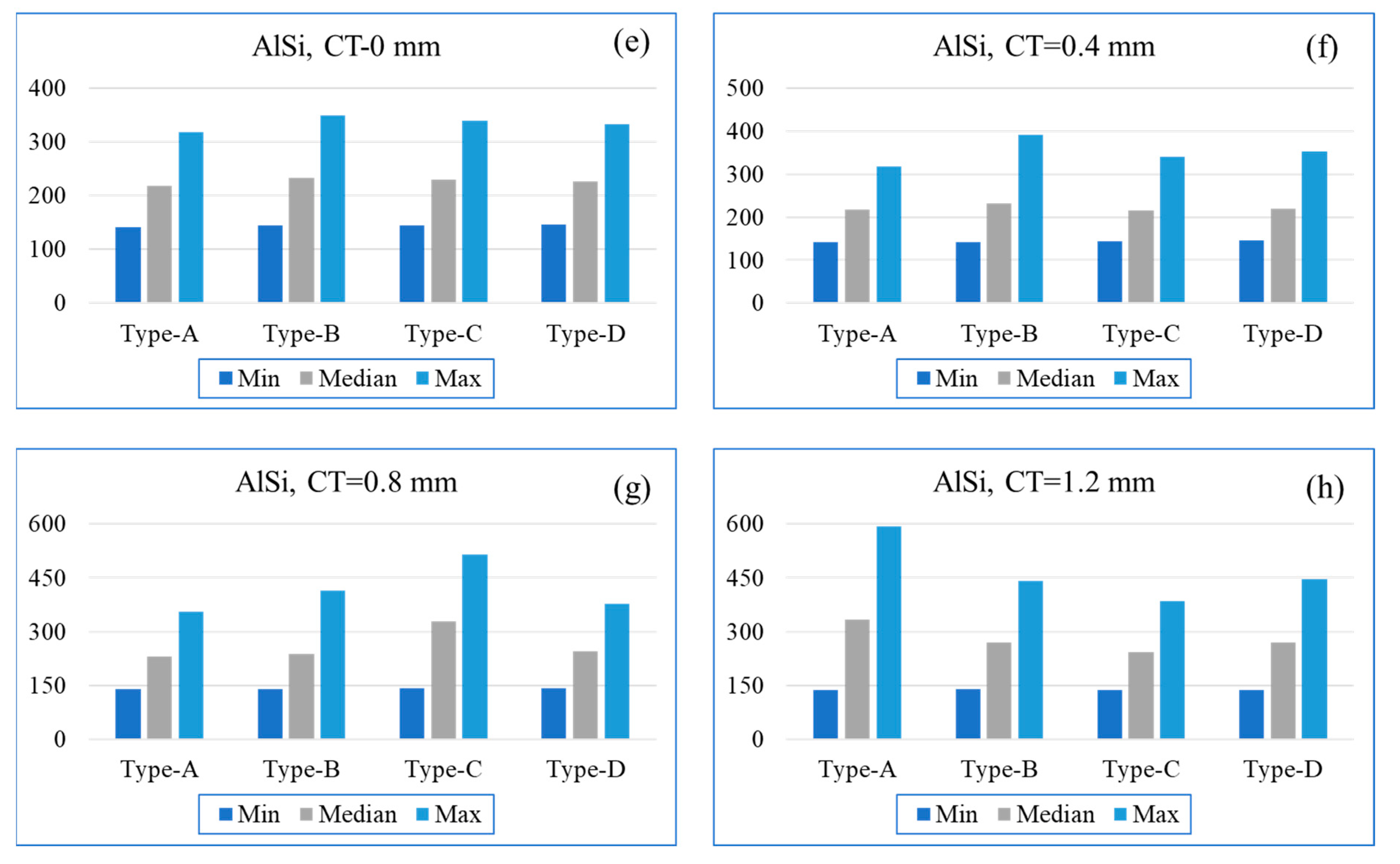
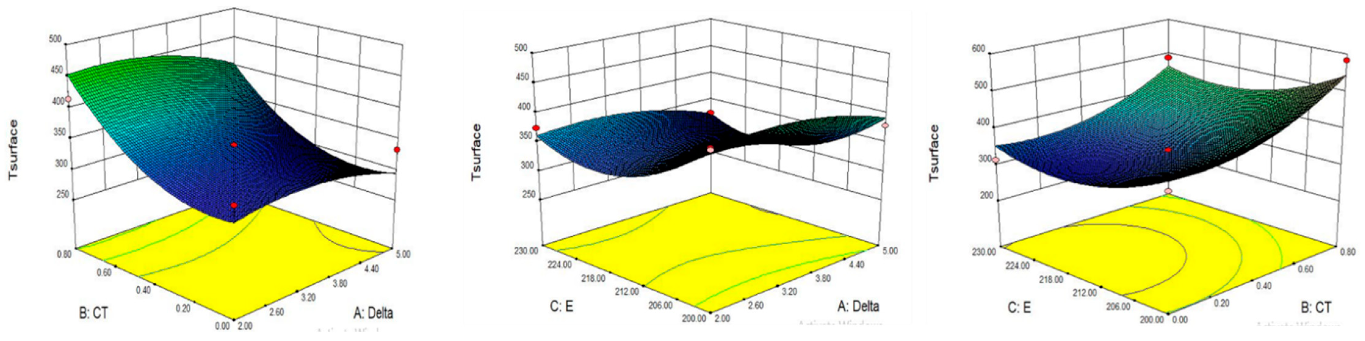
8.3. Effect on Surface Temperature
8.4. Optimization of Parameter
9. Conclusions
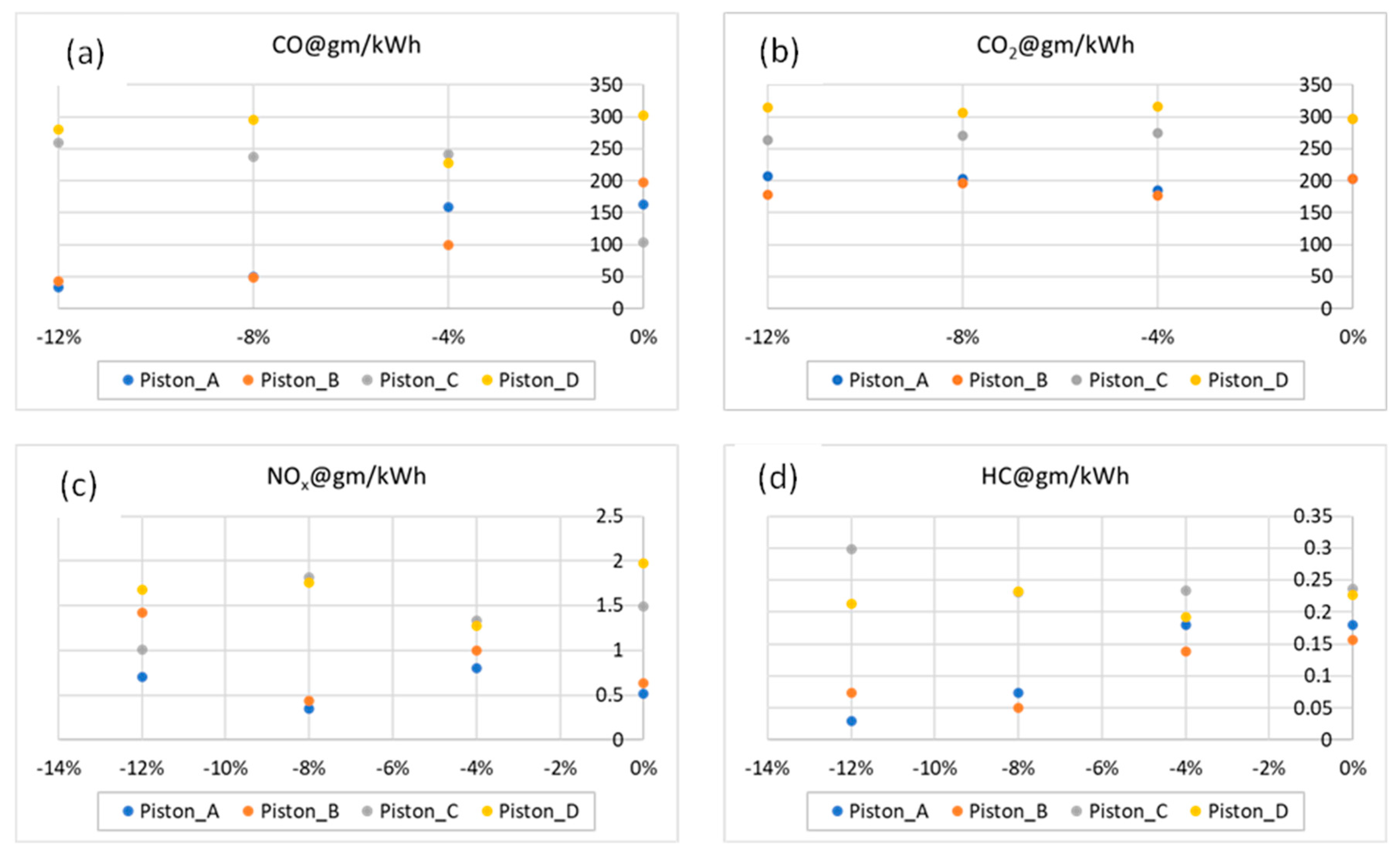
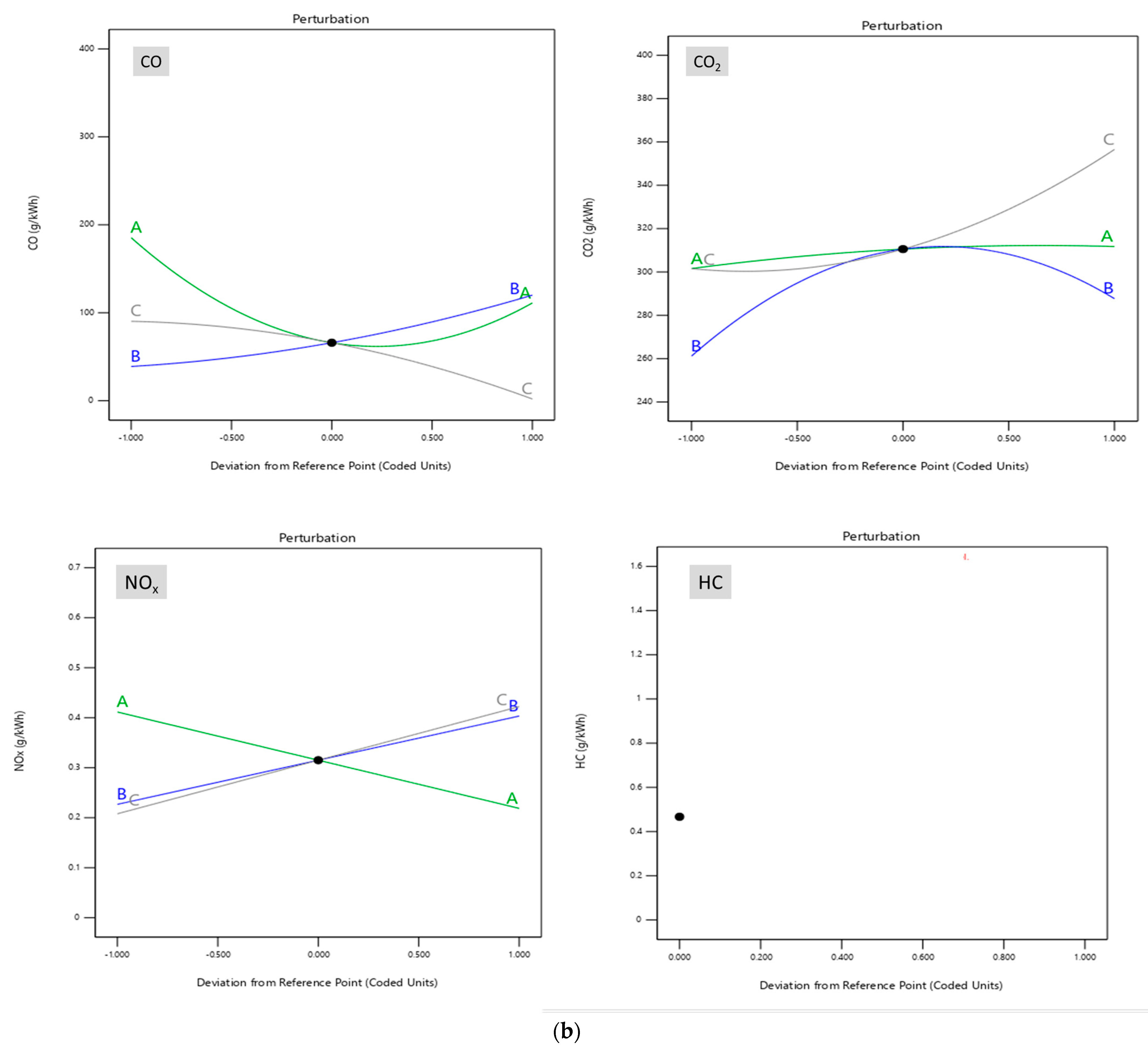
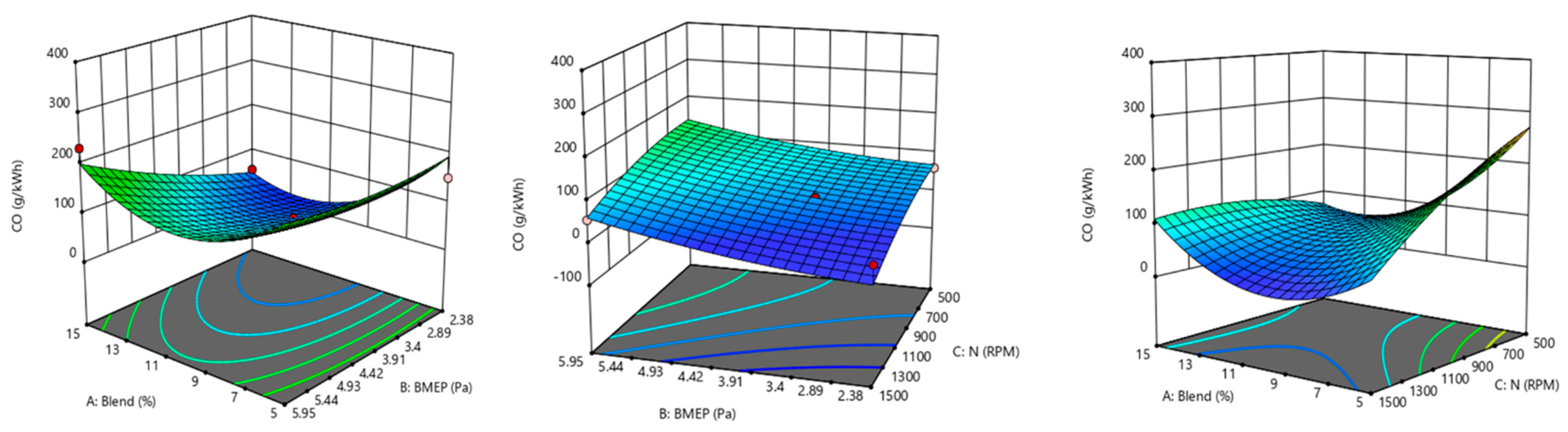
- Piston type_D has a maximum CO emission of 300 gm/kWh at −8% decarbonization, while type_A and type_B have the lowest CO emission level of 50 gm/kWh at −12% decarbonization using the B15 blend.
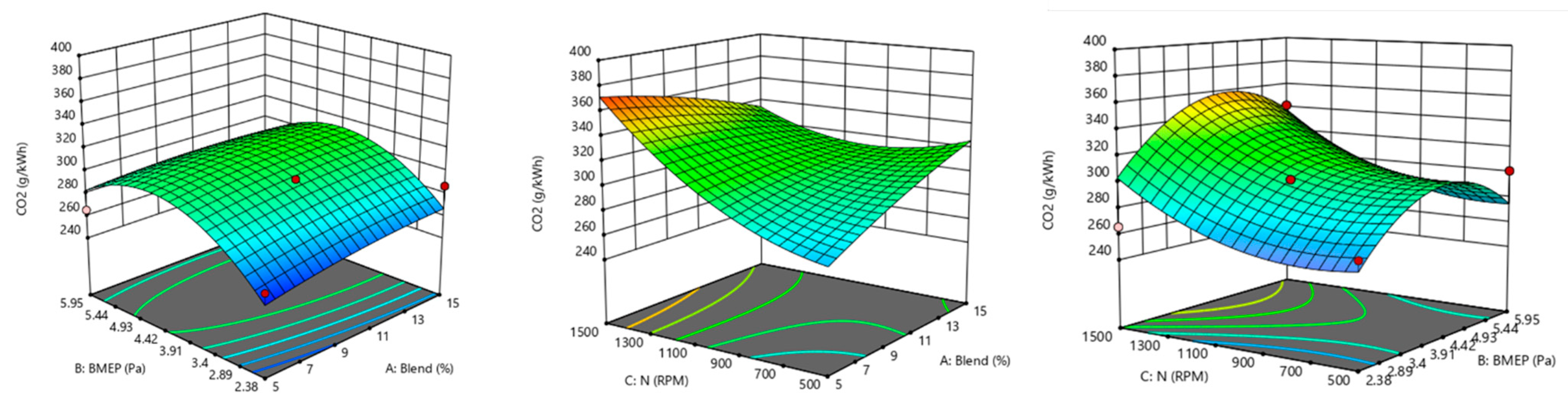
- At −12% decarbonization, the type_B design has thelowestCO2 emission of 175 gm/kWh among all designs considered.
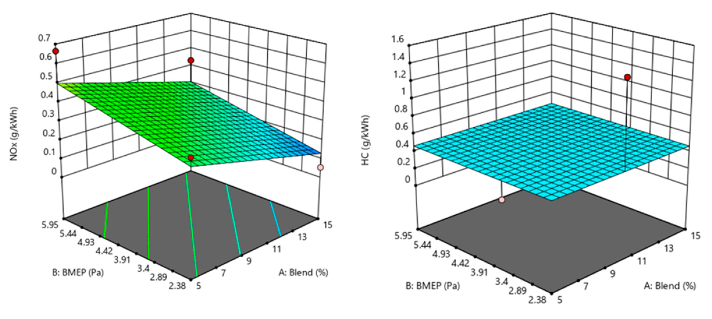
- For both piston designs, type_A and type_B, the NOx emission is lowest at −8% decarbonization through blending.
- Overall, it is observed that the type_A and type_B designs are more efficient compared to other designs in mitigation emission through blend replacement and design exchange.
Supplementary Materials
Author Contributions
Funding
Acknowledgments
Conflicts of Interest
Abbreviations
| A:B,C | Independent variables |
| A/F | Air to fuel ratio |
| AlSi | Alloy of Aluminum and Silicon |
| APPSY | Measurement software for dynamometer |
| ASTM | American standard of testing and Method |
| B5/B10/B15 | Gasoline methanol blend with 5%, 10%, and 15% methanol |
| BMEP | Break mean effective pressure |
| CO | Carbon monoxide |
| CO2 | Carbon dioxide |
| CAD | Computer aided drafting |
| CT | Coating thickness |
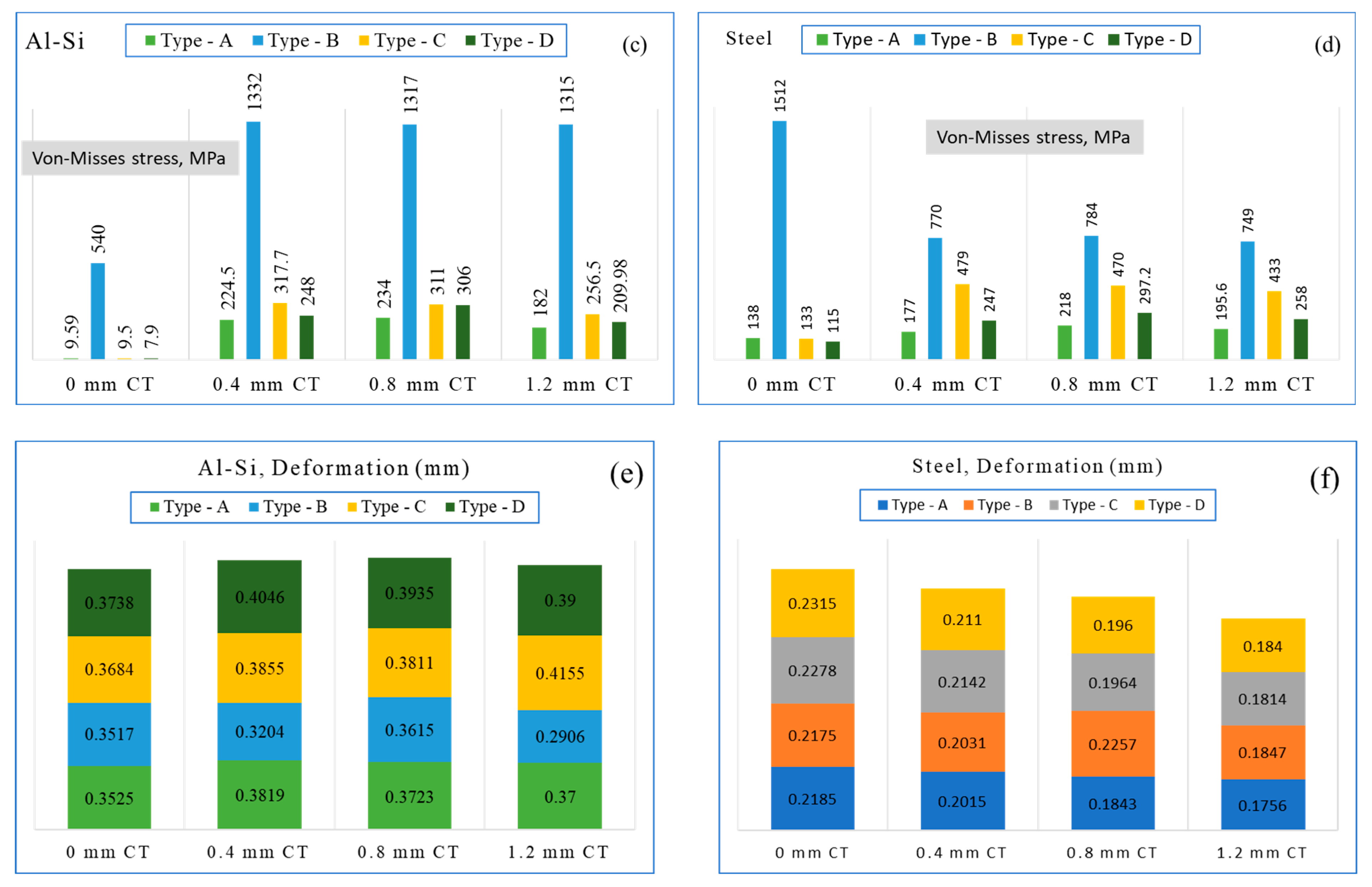
| Delastic | Elastic deformation |
| FEA | Finite element analysis |
| FGM | Functionally graded material |
| HC | Hydrocarbon |
| HP | Horse power |
| kWh | Kilo watt hour |
| MgZrO3 | Magnesium Zirconate |
| MON | Motor octane number |
| NDIR | Non-dispersive infrared |
| NOx | Nitrogen oxide |
| NiCrAl | Nickle, Chromium, and Aluminum alloy |
| O2 | Oxygen |
| OCT | Octane number |
| PCI | Peripheral component interconnect |
| PVD | Physical vapor deposition |
| RON | Research octane number |
| RSM | Response surface methodology |
| Tsurface | Surface temperature |
| σvon-Mises | vonMises stress |
| ρ | density |
| κ | Kinetic viscosity |
| ν | Specific volume |
References
- Carley, S.; Evans, T.P.; Graff, M.; Konisky, D.M. A framework for evaluating geographic disparities in energy transition vulnerability. Nat Energy 2018, 3, 621–627. [Google Scholar] [CrossRef]
- Grubler, A.; Wilson, C.; Bento, N.; Boza-Kiss, B.; Krey, V.; Mccollum, D.L.; Rao, N.D.; Riahi, K.; Rogelj, J.; De Stercke, S.; et al. A low energy demand scenario for meeting the 1.5 °C target and sustainable development goals without negative emission technologies. Nat. Energy 2018, 3, 515–527. [Google Scholar] [CrossRef]
- Sgouridis, S.; Carbajales-Dale, M.; Csala, D.; Chiesa, M.; Bardi, U. Comparative net energy analysis of renewable electricity and carbon capture and storage. Nat. Energy 2019, 4, 456–465. [Google Scholar] [CrossRef]
- Farmer, H.O. Free-piston compressor-engines. Nature 1947, 159, 413. [Google Scholar] [CrossRef]
- He, W. The Future Development of the Internal-Combustion Engine. Nature 1918, 102, 307–308. [Google Scholar] [CrossRef]
- Powdered Fuel: Progress and Prospects. Nature 1939, 144, 774–775. [CrossRef]
- Markard, J. The next phase of the energy transition and its implications for research and policy. Nat. Energy 2018, 3, 628–633. [Google Scholar] [CrossRef]
- Brockway, P.E.; Owen, A.; Brand-Correa, L.I.; Hardt, L. Estimation of global final-stage energy-return-on-investment for fossil fuels with comparison to renewable energy sources. Nat. Energy 2019, 4, 612–621. [Google Scholar] [CrossRef]
- Raimi, D.; Carley, S.; Konisky, D. Mapping county-level vulnerability to the energy transition in US fossil fuel communities. Sci. Rep. 2022, 12, 15748. [Google Scholar] [CrossRef]
- King, L.C.; van den Bergh, J.C.J.M. Implications of net energy-return-on-investment for a low-carbon energy transition. Nat. Energy 2018, 3, 334–340. [Google Scholar] [CrossRef] [Green Version]
- Mishra, P.C.; Ishaq, R.B.; Khoshnaw, F. Mitigation Strategy of Carbon Dioxide Emissions through Multiple Muffler design exchange and Gasoline-Methanol blend replacement. J. Clean. Prod. 2020, 286, 125460. [Google Scholar] [CrossRef]
- Mishra, P.C.; Gupta, A.; Kumar, A.; Bose, A. Methanol and petrol blended alternate fuel for future sustainable engine: A performance and emission analysis. Measurement 2020, 155, 107519, Corrigendum in Measurement 2022, 199, 111542. [Google Scholar] [CrossRef]
- Al-Farayedhi, A.A.; Al-Dawood, A.M.; Gandhidasan, P. Effects of Blending MTBE with Unleaded Gasoline on Exhaust Emissions of SI Engine. J. Energy Resour. Technol. 2000, 122, 239–247. [Google Scholar] [CrossRef]
- Abeydeera, L.H.U.W.; Mesthrige, J.W.; Samarasinghalage, T.I. Global Research on Carbon Emissions: A Scientometric Review. Sustainability 2019, 11, 3972. [Google Scholar] [CrossRef]
- Anenberg, S.; Miller, J.; Minjares, R.; Du, L.; Henze, D.K.; Lacey, F.; Malley, C.S.; Emberson, L.; Franco, V.; Klimont, Z.; et al. Impacts and mitigation of excess diesel-related NOx emissions in 11 major vehicle markets. Nature 2017, 545, 467–471. [Google Scholar] [CrossRef] [PubMed]
- Verhelst, S.; Turner, J.W.; Sileghem, L.; Vancoillie, J. Methanol as a fuel for internal combustion engines. Prog. Energy Combust. Sci. 2019, 70, 43–88. [Google Scholar] [CrossRef]
- Yao, Y.; Chang, Y.; Huang, R.; Zhang, L.; Masanet, E. Environmental implications of the methanol economy in China: Well-to-wheel comparison of energy and environmental emissions for different methanol fuel production pathways. J. Clean. Prod. 2018, 172, 1381–1390. [Google Scholar] [CrossRef]
- Riaz, A.; Zahedi, G.; Klemeš, J.J. A review of cleaner production methods for the manufacture of methanol. J. Clean. Prod. 2013, 57, 19–37. [Google Scholar] [CrossRef]
- Nguyen, T.B.; Zondervan, E. Methanol production from captured CO2 using hydrogenation and reforming technologies_ environmental and economic evaluation. J. CO2 Util. 2019, 34, 1–11. [Google Scholar] [CrossRef]
- Masum, B.; Masjuki, H.; Kalam, M.; Palash, S.; Habibullah, M. Effect of alcohol–gasoline blends optimization on fuel properties, performance and emissions of a SI engine. J. Clean. Prod. 2015, 86, 230–237. [Google Scholar] [CrossRef] [Green Version]
- Wang, Y.; Lin, L.; Roskilly, A.P.; Zeng, S.; Huang, J.; He, Y.; Huang, X.; Huang, H.; Wei, H.; Li, S.; et al. An analytic study of applying Miller cycle to reduce NOx emission from petrol engine. Appl. Therm. Eng. 2007, 27, 1779–1789. [Google Scholar] [CrossRef]
- Mishra, P.C.; Kar, S.K.; Mishra, H. Effect of perforation on exhaust performance of a turbo pipe type muffler using methanol and gasoline blended fuel: A step to NOx control. J. Clean. Prod. 2018, 183, 869–879. [Google Scholar] [CrossRef]
- Baker, R.A., Sr.; Doerr, R.C. Catalytic Reduction of Nitrogen Oxides in Automobile Exhaust. J. Air Pollut. Control Assoc. 1964, 14, 409–414. [Google Scholar] [CrossRef] [PubMed]
- Esfahanian, V.; Javaheri, A.; Ghaffarpour, M. Thermal analysis of an SI engine piston using different combustion boundary condition treatments. Appl. Therm. Eng. 2006, 26, 277–287. [Google Scholar] [CrossRef]
- Liu, Y.; Reitz, R.D. Multidimensional Modelling of Combustion Chamber Surface Temperatures; SAE Technical Paper 971593; SAE: Warrendale, PA, USA, 1997. [Google Scholar] [CrossRef]
- Buyukkaya, E. Thermal analysis of functionally graded coating AlSi alloy and steel pistons. Surf. Coatings Technol. 2008, 202, 3856–3865. [Google Scholar] [CrossRef]
- Taymaz, I.; Çakır, K.; Mimaroglu, A. Experimental study of effective efficiency in a ceramic coated diesel engine. Surf. Coatings Technol. 2005, 200, 1182–1185. [Google Scholar] [CrossRef]
- Taymaz, I. The effect of thermal barrier coatings on diesel engine performance. Surf. Coatings Technol. 2007, 201, 5249–5252. [Google Scholar] [CrossRef]
- Buyukkaya, E.; Cerit, M. Thermal analysis of a ceramic coating diesel engine piston using 3-D finite element method. Surf. Coatings Technol. 2007, 202, 398–402. [Google Scholar] [CrossRef]
- Yessian, S.; Varthanan, P.A. Optimization of Performance and Emission Characteristics of Catalytic Coated IC Engine with Biodiesel Using Grey-Taguchi Method. Sci. Rep. 2020, 10, 2129. [Google Scholar] [CrossRef] [Green Version]
- Verma, P.; Zare, A.; Jafari, M.; Bodisco, T.; Rainey, T.; Ristovski, Z.; Brown, R.J. Diesel engine performance and emissions with fuels derived from waste tyres. Sci. Rep. 2018, 8, 2457. [Google Scholar] [CrossRef]
- Ordouei, M.H.; Elkamel, A.; Dusseault, M.B.; Alhajri, I. New sustainability indices for product design employing environmental impact and risk reduction: Case study on gasoline blends. J. Clean. Prod. 2015, 108, 312–320. [Google Scholar] [CrossRef]
- Ou, S.; He, X.; Ji, W.; Chen, W.; Sui, L.; Gan, Y.; Lu, Z.; Lin, Z.; Deng, S.; Przesmitzki, S.; et al. Machine learning model to project the impact of COVID-19 on US motor gasoline demand. Nat. Energy 2020, 5, 666–673. [Google Scholar] [CrossRef]
- Zhou, N.; Khanna, N.; Feng, W.; Ke, J.; Levine, M. Scenarios of energy efficiency and CO2 emissions reduction potential in the buildings sector in China to year 2050. Nat. Energy 2018, 3, 978–984. [Google Scholar] [CrossRef]
- Figueredo, A.J.; Wolf, P.S. Assortative pairing and life history strategy—A cross-cultural study. Hum. Nat. 2009, 20, 317–330. [Google Scholar] [CrossRef]
- Hao, Z.; AghaKouchak, A.; Nakhjiri, N.; Farahmand, A. Global integrated drought monitoring and prediction system (GIDMaPS) data sets. Figshare 2014, 1, 140001. [Google Scholar] [CrossRef]
- Montgomery, D.C. Design and Analysis of Experiments. J. Am. Stat. Assoc. 2000, 16, 2. [Google Scholar]
- Wang, X.; Chen, H.; Liu, H.; Li, P.; Yan, Z.; Huang, C.; Zhao, Z.; Gu, Y. Simulation and optimization of continuous laser transmission welding between PET and titanium through FEM, RSM, GA and experiments. Opt. Lasers Eng. 2013, 51, 1245–1254. [Google Scholar] [CrossRef]
- Zhang, Z.; Tian, J.; Xie, G.; Li, J.; Xu, W.; Jiang, F.; Huang, Y.; Tan, D. Investigation on the combustion and emission characteristics of diesel engine fueled with diesel/methanol/n-butanol blends. Fuel 2022, 314, 123088. [Google Scholar] [CrossRef]
- Zhang, Z.; Li, J.; Tian, J.; Dong, R.; Zou, Z.; Gao, S.; Tan, D. Performance, combustion and emission characteristics investigations on a diesel engine fueled with diesel/ethanol/n-butanol blends. Energy 2022, 249, 123733. [Google Scholar] [CrossRef]


| Measured Quantity | Measurement Range | Accuracy | Type of Instrument | % Uncertainty |
|---|---|---|---|---|
| Load | ±90 Nm | ±0.1 Nm | Strain gauge type load cell | ±0.1 Nm |
| Speed | 0–7000 rpm | ±1 rpm | Magnetic pick-up type speed sensor | ±0.1 rpm |
| Time | - | ±0.1 s | - | ±0.2 s |
| CO | 0–10% by vol | ±0.001% | Non-dispersive infrared gas sensor | ±1 |
| CO2 | 0–20% by vol | ±0.001% | Non-dispersive infrared gas sensor | ±1 |
| NOx | 0–5000 ppm | ±1 ppm | Electro chemical gas sensor | ±0.6 |
| EGT | 0–900°C | ±0.3 °C | K-type thermo-couple | ±0.1 |
| Materials | Thermal Conductivity (W/m °C) | Density (kg/m3) | Specific Heat (J/kg °C) |
|---|---|---|---|
| Piston (AlSi) | 155 | 2700 | 960 |
| Piston (Steel) | 79 | 7870 | 500 |
| Bond coat (100%NiCrAl) | 16.1 | 7870 | 764 |
| 100%MgZrO3 | 0.8 | 5600 | 650 |
| 70%MgZrO3+30%NiCrAl | 4.6 | 6130.4 | 676.6 |
| 50%MgZrO3+50%NiCrAl | 7.3 | 6543.7 | 697.39 |
| 30%MgZrO3+70%NiCrAl | 10.4 | 7016.7 | 721.14 |
| Rings (cast iron) | 16 | 7200 | 460 |
| Sl. No. | Material | Temperature (°C) at Crown Centre [14] | Temperature (°C) at Crown Centre (Current) | Difference in Temperature | Temperature (°C) at Bowl Rim [14] | Temperature (°C) at Bowl Rim (Current) | Difference in Temperature |
|---|---|---|---|---|---|---|---|
| 1 | Steel (UC) | 333 | 357 | 7.20% | 357 | 372 | 4.20% |
| 2 | Steel (CT-0.4 mm) | 388 | 379 | −4.12% | 418 | 422 | 0.96% |
| 3 | AlSi (UC) | 285 | 325 | 14% | 270 | 315 | 16.67% |
| 4 | AlSi (CT-0.4 mm) | 342 | 358 | 4.6% | 366 | 380 | 3.82% |
| Variables | Symbol | Unit | Level | ||
|---|---|---|---|---|---|
| −1 | 0 | 1 | |||
| δ | A1 | mm | 2 | 3.5 | 5 |
| CT | B1 | mm | 0 | 0.4 | 0.8 |
| E | C1 | GPa | 200 | 215 | 230 |
| Blend | A2 | % | 5 | 3.5 | 15 |
| BMEP | B2 | bar | 2.98 | 3.57 | 5.95 |
| N | C2 | rpm | 500 | 1000 | 1500 |
| Run | δ | CT | E | Delastic | σvon-Mises | Tsurface | |||
|---|---|---|---|---|---|---|---|---|---|
| Actual | Predicted | Actual | Predicted | Actual | Predicted | ||||
| 1 | 5 | 0.8 | 215 | 0.3935 | 0.3891 | 306 | 158.38 | 379 | 404.63 |
| 2 | 3.5 | 0.4 | 215 | 0.3855 | 0.3855 | 317.7 | 317.7 | 341 | 341 |
| 3 | 2 | 0.4 | 230 | 0.3872 | 0.3812 | 872 | 755.75 | 375 | 361.75 |
| 4 | 5 | 0.4 | 200 | 0.211 | 0.217 | 247 | 363.25 | 379 | 392.25 |
| 5 | 5 | 0.4 | 230 | 0.4345 | 0.424 | 232 | 309.5 | 324 | 323.5 |
| 6 | 2 | 0.8 | 215 | 0.3615 | 0.3526 | 678 | 724.13 | 415 | 453.38 |
| 7 | 3.5 | 0.8 | 200 | 0.1964 | 0.1948 | 470 | 501.38 | 582 | 543.13 |
| 8 | 3.5 | 0 | 230 | 0.3874 | 0.389 | 234 | 202.62 | 315 | 353.88 |
| 9 | 3.5 | 0.4 | 215 | 0.3855 | 0.3855 | 317.7 | 317.7 | 341 | 341 |
| 10 | 5 | 0 | 215 | 0.3738 | 0.3827 | 79 | 32.88 | 333 | 294.63 |
| 11 | 2 | 0 | 215 | 0.3684 | 0.3728 | 95 | 242.62 | 340 | 314.38 |
| 12 | 3.5 | 0.4 | 215 | 0.3855 | 0.3855 | 317.7 | 317.7 | 341 | 341 |
| 13 | 3.5 | 0.4 | 215 | 0.3855 | 0.3855 | 317.7 | 317.7 | 341 | 341 |
| 14 | 3.5 | 0 | 200 | 0.2278 | 0.2129 | 133 | 62.87 | 379 | 404.13 |
| 15 | 2 | 0.4 | 200 | 0.2031 | 0.2136 | 770 | 692.5 | 422 | 422.5 |
| 16 | 3.5 | 0.4 | 215 | 0.3855 | 0.3855 | 317.7 | 317.7 | 341 | 341 |
| 17 | 3.5 | 0.8 | 230 | 0.3785 | 0.3934 | 301 | 371.13 | 489 | 463.88 |
| Run | Blend | BMEP | N | CO | CO2 | NOx | HC | ||||
|---|---|---|---|---|---|---|---|---|---|---|---|
| Actual | Predicted | Actual | Predicted | Actual | Predicted | Actual | Predicted | ||||
| 1 | 10 | 2.38 | 500 | 59.8401 | 67.97 | 264.035 | 256.31 | 264.035 | 0.1196 | 0.584848 | 0.4668 |
| 2 | 5 | 3.57 | 500 | 311.061 | 272.37 | 247.533 | 260.61 | 247.533 | 0.2748 | 1.05007 | 0.4668 |
| 3 | 5 | 2.38 | 1000 | 149.87 | 193.32 | 257.688 | 247.97 | 257.688 | 0.3231 | 0.618078 | 0.4668 |
| 4 | 10 | 3.57 | 1000 | 53.91 | 53.91 | 302.117 | 302.12 | 302.117 | 0.2856 | 0.212672 | 0.4668 |
| 5 | 10 | 3.57 | 1000 | 53.91 | 53.91 | 302.117 | 302.12 | 302.117 | 0.2856 | 0.212672 | 0.4668 |
| 6 | 5 | 5.95 | 1000 | 210.788 | 204.62 | 265.305 | 282.94 | 265.305 | 0.4997 | 1.09659 | 0.4668 |
| 7 | 15 | 5.95 | 1000 | 231.274 | 200.25 | 272.286 | 284.64 | 272.286 | 0.3069 | 0.578202 | 0.4668 |
| 8 | 15 | 3.57 | 500 | 53.3709 | 51.97 | 299.578 | 320.57 | 299.578 | 0.0821 | 0.219318 | 0.4668 |
| 9 | 10 | 5.95 | 1500 | 55.5273 | 60.76 | 341.469 | 337.83 | 341.469 | 0.5105 | 0.16615 | 0.4668 |
| 10 | 10 | 2.38 | 1500 | 15.6339 | −29.69 | 265.305 | 303.01 | 265.305 | 0.3339 | 1.47541 | 0.4668 |
| 11 | 15 | 3.57 | 1500 | 44.7453 | 83.43 | 338.93 | 325.85 | 338.93 | 0.2964 | 0.186088 | 0.4668 |
| 12 | 10 | 5.95 | 500 | 107.82 | 139.78 | 300.848 | 274.5 | 300.848 | 0.2961 | 0.252548 | 0.4668 |
| 13 | 5 | 3.57 | 1500 | 56.6055 | 58.01 | 380.82 | 359.82 | 380.82 | 0.4891 | 0.259194 | 0.4668 |
| 14 | 15 | 2.38 | 1000 | 55.5273 | 49.27 | 286.884 | 266.61 | 286.884 | 0.1304 | 0.385468 | 0.4668 |
| 15 | 10 | 3.57 | 1000 | 53.91 | 53.91 | 302.117 | 302.12 | 302.117 | 0.2856 | 0.212672 | 0.4668 |
| 16 | 10 | 3.57 | 1000 | 53.91 | 53.91 | 302.117 | 302.12 | 302.117 | 0.2856 | 0.212672 | 0.4668 |
| 17 | 10 | 3.57 | 1000 | 53.91 | 53.91 | 302.117 | 302.12 | 302.117 | 0.2856 | 0.212672 | 0.4668 |
| Parameter | Aim | Lower Limit | Upper Limit |
|---|---|---|---|
| δ | Within range | 2 mm | 5 mm |
| CT | Within range | 0 mm | 0.8 mm |
| E | Within range | 200 GPa | 230 GPa |
| Delastic | Minimize | 0.1964 mm | - |
| Σvon-Mises | Maximize | - | 872 GPa |
| Tsurface | Minimize | 315 °C | - |
| Sl. | Output Parameter | δ | CT | E | Predicted Value | Simulation Value | % Error |
|---|---|---|---|---|---|---|---|
| 1 | Delastic | 2.16 | 0.15 | 216.64 | 0.1964 mm | 0.1922 mm | 0.0042 |
| 2 | σvon-Mises | 3.79 | 0.18 | 214.64 | 872 GPa | 871.65 GPa | 0.35 |
| 3 | Tsurface | 4.27 | 0.37 | 218.16 | 315 °C | 314.1 °C | 0.9 |
Publisher’s Note: MDPI stays neutral with regard to jurisdictional claims in published maps and institutional affiliations. |
© 2022 by the authors. Licensee MDPI, Basel, Switzerland. This article is an open access article distributed under the terms and conditions of the Creative Commons Attribution (CC BY) license (https://creativecommons.org/licenses/by/4.0/).
Share and Cite
Mishra, P.C.; Gupta, A.; Samanta, S.; Ishaq, R.B.; Khoshnaw, F. Framework for Energy-Averaged Emission Mitigation Technique Adopting Gasoline-Methanol Blend Replacement and Piston Design Exchange. Energies 2022, 15, 7188. https://doi.org/10.3390/en15197188
Mishra PC, Gupta A, Samanta S, Ishaq RB, Khoshnaw F. Framework for Energy-Averaged Emission Mitigation Technique Adopting Gasoline-Methanol Blend Replacement and Piston Design Exchange. Energies. 2022; 15(19):7188. https://doi.org/10.3390/en15197188
Chicago/Turabian StyleMishra, Prakash Chandra, Anand Gupta, Saikat Samanta, Rihana B. Ishaq, and Fuad Khoshnaw. 2022. "Framework for Energy-Averaged Emission Mitigation Technique Adopting Gasoline-Methanol Blend Replacement and Piston Design Exchange" Energies 15, no. 19: 7188. https://doi.org/10.3390/en15197188