Abstract
In this paper, an improved probabilistic roadmap (IPRM) algorithm is proposed to solve the energy consumption problem of multi-unmanned aerial vehicle (UAV) path planning with an angle. Firstly, in order to simulate the real terrain environment, a mathematical model was established; secondly, an energy consumption model was established; then, the sampling space of the probabilistic roadmap (PRM) algorithm was optimized to make the obtained path more explicit and improve the utilization rate in space and time; then, the sampling third-order B-spline curve method was used to curve the rotation angle to make the path smoother and the distance shorter. Finally, the results of the improved genetic algorithm (IGA), PRM algorithm and IPRM algorithm were compared through a simulation. The data analysis shows that the IGA has significant advantages over other algorithms in some aspects, and can be well applied to the path planning of UAVs.
1. Introduction
In recent years, the UAV has been developed rapidly and has been used in many industries due to the advantages of being small, light, flexible and cheap to manufacture, such as disaster rescue, panoramic photography, plant protection operations and wildlife protection [1]. In plant protection work, the UAV plays a vital role in crop production to ensure that it can help farmers to more conveniently perform spraying, fertilization, pollination, etc., due to the fact that it has a high speed, high efficiency, low cost and the advantage of spraying evenly. Regarding the orientation of national policy, the scale of planting has become a trend and there is a growing number of plant protection tasks using UAVs [2]. In addition, UAV technology has been used for archeology [3,4,5] or for the mapping of magnetic fields [6,7]. Due to the short endurance time of civil UAVs, different information acquisition paths require different operation times when using UAVs for mountain surveillance. Therefore, UAV path planning is the key problem when obtaining information in mountain forest monitoring.
The path planning of UAVs is a hot topic in the UAV research field [8]. At present, there has been a large amount of research in this field. The task of path planning is to find a path from the start point to avoid all obstacles and reach the target point. Common algorithms include the gray wolf algorithm [9,10], ant colony algorithm [11,12], particle swarm optimization algorithm [13,14], A* algorithm [15,16], RRT algorithm [17] and genetic algorithm [18,19]. Table 1 shows the UAV path planning methods and algorithms used in many papers. For this paper, the PRM algorithm was adapted in order to solve the complex path planning problem in a high-dimensional space. The composition stage of the PRM algorithm is based on random sampling used to construct a random path graph, which is the core idea of the algorithm. Compared with other planning problems, the random sampling method avoids the problem of large computation in a high-dimensional space, and makes it possible to deal with complex path planning problems in a high-dimensional space.

Table 1.
UAV path planning methods.
The applications of UAVs take place in a number of different scenarios. References [20,21,22,23,24,25] describe implementation issues of UAV technology in various scenarios. In [20], the UAV is a very useful and effective tool for improving the capacity of disaster situational awareness for responders. The UAV path planning is modeled as an optimization problem, where the fitness function includes the UAV’s flight distance and risk, and three constraints include the UAV height, UAV angle and limited UAV slope. Reference [21] deals with multi-UAV systems, forming aerial networks, mainly employed to provide internet connectivity and different network services to ground users. UAV base station (UAV-BS) development plays a major part in rescue operations and post-disaster reconstruction. Improving the network throughput in the UAV-BS signal coverage area and reducing deployment costs while maintaining effective communication are important issues in [22]. Due to the limited ability of the UAV itself, it is difficult to complete large-scale combat tasks. The multi-UAV has an overall combat capability, which is an important way to solve the problem of large-scale combat tasks in [23]. In [24], UAV technology is used to develop a fast and energy-efficient multi-rotor UAV global planner to support personnel operations in rescue missions. In [25], solving the path planning problem of a UAV is a challenging issue, especially if there are too many checkpoints to visit. The brute force approach is mainly used to find the shortest path in the mission area, which requires too much time to find a solution. Therefore, the application scenarios of UAVs are diverse, and the path planning of UAVs is very worthy of in-depth study.
2. Related Works
The PRM algorithm was proposed in 1996 by Latombe people to solve high-dimensional space such as the complex motion planning problem of the random method [26]. It is by far the most successful and most popular motion planning method based on random sampling. One of the PRM algorithms are usually divided into two phases: composition and query. The phase composition based on a random sampling random path diagram is the core of the algorithm. Compared with other planning algorithms, the random sampling method avoids the modeling and description process of high-dimensional space, solves the problem of an “exponential explosion” and makes it possible to deal with complex motion planning problems in high-dimensional space. In the query stage, a variety of mature graph search algorithms can be selected according to the needs. The PRM algorithm has two application forms: single-query planning and multi-query planning. Single-query planning regenerates a roadmap every time, including its expansion randomized potential planner algorithm, etc. [27]. Multi-query planning generates a roadmap for multiple planning. A single query is used for small-scale dynamic planning, and multiple queries are used for multi-machine collaborative planning. It can be used for large-range static planning.
In recent years, the research on the sampling strategy of the PRM algorithm has been greatly developed. In [28], the sampling probabilistic roadmap algorithm is used to plan the UAV track, and the obstacle boundary points are taken as the sampling points to reduce the sampling area and improve the sampling efficiency. However, it does not consider that the actual UAV needs a reserved distance for the corner. In [29], a genetic algorithm and PRM algorithm are, respectively, used to plan the path of the map, and the advantages and disadvantages of the two algorithms are compared. Although the effect of the genetic algorithm is better, it consumes a greater operation time. In [30], scholars propose an improved PRM algorithm method used to enhance the sampling by intelligently detecting which areas of the configuration space are easy and which parts are not. The algorithm then biases the sampling only to the difficult areas that may contain narrow passages. In [31], scholars propose a new, simple sampling strategy called the Gaussian sampler. However, some of the samples obtained through this method have no effect on improving the connectivity of the roadmap. In [32], scholars propose an improved PRM algorithm used to increase the effective sampling point density. However, it also has the disadvantages of a lower efficiency, longer running time and longer planned path.
To sum up, the PRM algorithm is becoming more and more intelligent in terms of drawing, which mainly considers the strategy of random sampling and the design of the local planner. At the same time, it also has some problems in improving the traditional PRM algorithm, such as: the operation efficiency is low, the path is too long and the obstacles are not reasonably avoided. Therefore, in order to solve the above shortcomings, this paper presents an IPRM algorithm used to solve the path planning problem of UAVs with angular energy consumption. Firstly, a three-dimensional map model of a simulated mountain forest was established and an energy consumption forecast model was proposed for the angle. Then, an improved PRM algorithm was proposed to optimize the original sampling space and improve the operation efficiency; then, the third-order B-spline curve method [33] was used to optimize the angle; and then, the cost function in the PRM algorithm was improved by considering energy consumption. Finally, the experimental comparison proves that the proposed improved algorithm is better than other algorithms, and has good adaptability and a higher efficiency.
3. Establishment of Model
UAV path planning first needs to extract location information from the map. According to the map model in [34], the position, slope and height of each peak were randomly generated in this paper. The mathematical model can be expressed as:
where, and are the central coordinates of the i-th mountain; is the height value of the point corresponding to the horizontal point; and are the attenuation amount and control slope of the i-th peak along the x-axis and y-axis direction, respectively; and n represents the total number of peaks. The environment model is shown in Figure 1.
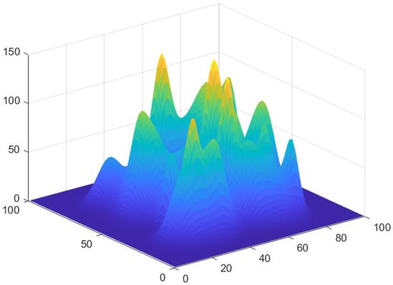
Figure 1.
Environment model.
Generally, in the research of the energy consumption optimization of UAVs, the distance of the path is used as the variable of energy consumption, and the energy consumption of UAVs is estimated by calculating the distance value. However, there are some other variables that will affect the energy consumption. In this paper, the energy consumption of UAVs was estimated by the characteristic variable of the fusion angle and distance factors. As shown in Figure 2, the UAV flies from node A to node C along an arc, where the arc angle is and the radius is . The angular velocity is calculated by using Equation (2). The arc length is calculated by using Equation (3). When the UAV is in yaw motion, the influence of external factors is not considered. It is considered that the UAV is in hovering state and the rotation angle speed is constant when it rotates. At this time, the external force and external torque of the UAV are zero. It is assumed that the angular velocity of the UAV is and the power is during yaw; then, the yaw energy efficiency coefficient of the UAV is shown in Equation (4). is the ratio of the path distance and energy consumption in the turning process of the UAV. v is the average speed of the UAV in the turning process; t1 is the time consumed in the turning process of the UAV; L is the arc length during the turn of the UAV.
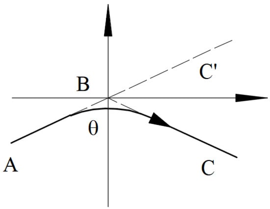
Figure 2.
Corner route.
In order to simulate the movement force model of the UAV, it was assumed that there is no natural wind in the environment; that is, there is no external force in the horizontal direction. In order to simplify the force model, the complex movement of the UAV was not considered, and only the movement force when moving forward and rising was considered to facilitate the calculation of the overall energy consumption, as shown in Figure 3.
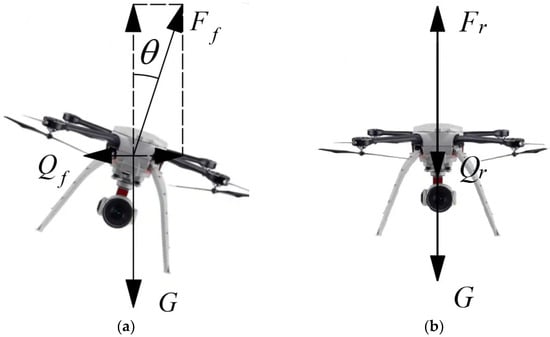
Figure 3.
Force analysis of motion for UAV: (a) force of forward movement; (b) force of rise.
G is the force of gravity received by the UAV as it moves. Gravitational acceleration and the mass of UAV is m. When the UAV flies in a straight line at uniform speed, the angle between the lift direction of the UAV and the weight line is , the lift force generated by the UAV is and the resistance generated by the air is . Since the UAV moves at a uniform speed, the resultant force on the UAV is zero. According to Figure 3a, the kinematics equations of a UAV flying in a straight line with uniform speed can be obtained as shown in Equations (5)–(7).
Assume that the power of the UAV is at this time, and the energy efficiency coefficient of the UAV when its horizontal moving speed is can be obtained; that is, the ratio of the energy consumption and flight distance during horizontal flight is shown in Equation (8). is the ratio of the path distance and energy consumption in the forward process of UAV. t2 is the time consumed by the horizontal movement of the UAV.
When the UAV rises in a straight line at uniform speed, the air resistance is opposite to its movement direction, which hinders the lift force of the UAV. According to Figure 3b, the kinematics equation of the UAV when it is rising at a uniform speed can be shown in Equation (9).
Assuming that the power of UAV is at this time, the energy efficiency coefficient of the UAV with vertical ascending velocity can be obtained; that is, the ratio of energy consumption during the ascending flight to the flight distance is shown in Equation (10). is the ratio of the path distance and energy consumption in the rise process of UAV. t3 is the time consumed during the rise of the UAV.
To sum up, the total energy consumption E of UAV can be calculated when various parameters and routes of UAV are known, as shown in Equation (10), where is the number of corners on the path and is the serial number of corners. Lf is the distance that the UAV moves horizontally; Lr is the distance that the UAV rises.
4. Approach for Path Planning
4.1. Traditional PRM Algorithm
The traditional PRM algorithm mainly consists of two stages: an offline learning stage and online planning stage [34].
In the offline learning stage, undirected path map is established. N random points are generated in space M to form node set V in the map. Then, the adjacent nodes are found for each node. The two points with obstacles on the straight path cannot be regarded as adjacent nodes. Finally, the set E of all edges is established. The undirected path map is shown in Figure 4a.
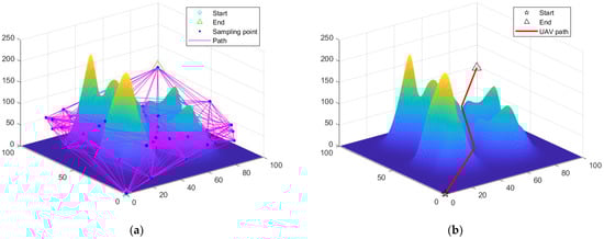
Figure 4.
Two stages of PRM algorithm: (a) offline learning stage; (b) online planning stage.
The task of the online planning stage is to connect the starting node with the target node by the edge generated from the first stage, and then to use the A* algorithm or other algorithms to find the shortest path on the path map, as shown in Figure 4b. Among them, the greater the number of sampling points N, the more accurate the final optimization result, and the greater the amount of calculations is.
4.2. Improved GA
Huang et al. [35] proposed an IGA to solve problems such as a slow convergence speed, falling into the local optimum easily, an unsmooth planning path and the high cost of the traditional genetic algorithm. The hybrid non-multi-string selection operator was proposed to expand the distribution range of the population and to avoid a premature convergence of the algorithm to some extent. An asymmetric mapping crossover operator and a heuristic multiple mutation operator were also proposed, which can accelerate convergence. Finally, a cubic B-spline curve was used to smooth the track. The specific effects are shown in Figure 5.
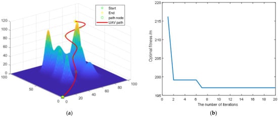
Figure 5.
IGA algorithm: (a) path graph; (b) curve of iteration.
4.3. Improved PRM
4.3.1. Optimize Sampling Space
This paper proposes a method for improving the PRM algorithm by reducing the space generated by random nodes while maintaining the number of random nodes, so as to improve the space utilization of the proposed IPRM algorithm. The specific operation is as follows: the range generated by the random node is reduced to an ellipse focusing on the starting node and the ending node, as shown in Figure 6. The obstacle shadows represent mountains, the sampling space represents the entire map and IPRM randomly generates small nodes.
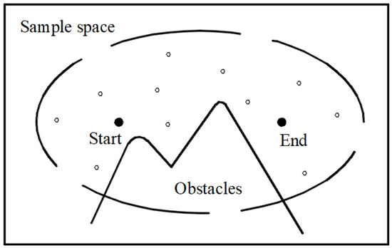
Figure 6.
Optimized sampling space.
The effect after sampling space optimization is shown in Figure 7. The IPRM algorithm adjusts the size and position of the ellipsoid according to the starting point and ending point, which improves the efficiency and space utilization while keeping the number of sampling points unchanged and overcomes the problem of the efficiency of the traditional PRM algorithm being reduced when the path needs to pass through dense obstacles or narrow channels.
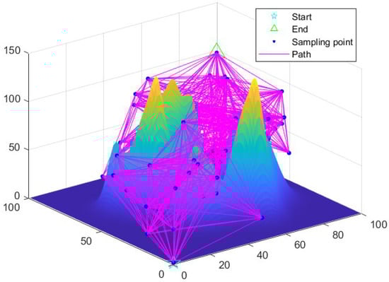
Figure 7.
The effect of sampling space optimization.
4.3.2. Optimizing Corner Path
In order to simulate the flight path of a UAV in the actual flight corner, this paper adopted the third-order B-spline curve method to optimize the trajectory path of the UAV. In order to ensure a certain distance between the B-spline and the obstacle, the radius of the fillet should be enlarged as far as possible, and the distance between the control points used by the B-spline should be self-adjusted, as shown in Figure 8. Obstacles represent the transverse section of the mountain. Figure 8 is the horizontal plane of the map. The red dotted line is obtained before B-spline processing, and the black curve is the path after B-spline processing.
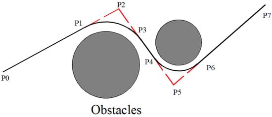
Figure 8.
Optimized angle.
Set the path nodes obtained by PRM algorithm as ; these nodes are used to define the trend and boundary range of spline curve. The B-spline curves of k-order are defined as follows:
is the k-order basis function of the ith B-spline, corresponding to node Pi, ; is the independent variable. The basis function has the following Debour–Cox recursive equation:
In this paper, the third-order quasi-uniform B-spline curve was adopted. The quasi-uniform B-spline curve retains the properties of the Bezier curve at the two endpoints; the tangent of the spline curve at the endpoint is the connecting line of the reciprocal two endpoints. The final effect is shown in Figure 9.
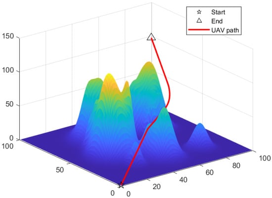
Figure 9.
The effect of angle optimization.
In order to determine the position of two points around the corner, first determine the radius of the fillet. The purpose is to reduce the path length and avoid contacting obstacles, so the position of the two points is very important. The following is the pseudo code used to simplify the implementation of an adaptive fillet radius:
- R = a; %R is a parameter in function B; let us set the radius of the fillet to an initial value.
- R’ = b;%Adjust by increasing or decreasing b meters each time; avoid path contact with obstacles.
- %If the height of the processed path is completely higher than the height of the obstacle, the radius of the rounded corner is reduced until it is close to the obstacle
- while B(path) > map %The function B is to B-spline the resulting path.
- R = R − R’;
- if B(path) < map
- R = R + R’;
- end
- end
- %If the height of the processed path is not exactly higher than the height of the obstacle, increase the radius of the fillet until it just exceeds the obstacle
- while B(path) < map
- R = R + R’;
- end
- path’ = function B(path); %path’ is the path that we need to get to.
4.3.3. Path Planning Considering Energy Consumption
In order to find a path with a shorter distance and lower energy consumption, this paper improves the traditional PRM by adding an energy consumption cost in the online planning stage, as shown in Equation (14):
g(n) is the cost of moving from the starting point to the node; h(n) is the estimated cost of moving from the node to the end point; k(n) is the coefficient of energy consumption, where, the higher it is, the higher the priority proportion of energy consumption is; e(n) is the energy consumption cost at the corner of moving from the starting point to the node.
4.4. Flowchart of IPRM
The flowchart of IPRM is shown in Figure 10.
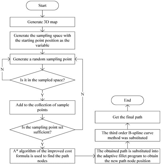
Figure 10.
Flowchart of IPRM.
5. Simulation Experiment and Result
In order to verify the effectiveness of the improved algorithm, this paper used MATLAB 2021b to carry out simulation experiments. The experimental environment was: Windows 10 family Chinese version; Processor AMD ryzen7 5700u with Radeon graphics 1.80 GHz and 16 GB memory. AMD ryzen7 5700u is a product of AMD Inc., a global semiconductor company headquartered in Santa Clara, California, USA. The map size was 100 × 100 × 100, the starting node was (1,1,1), the target node was (99,99,99) and the number of peaks was 20. The number of sampling points was 50. In this paper, a hexacopter with a 1.2 kg weight, 10,000 mAh battery capacity and 11.1 V voltage was selected for the simulation experiment. The average speed of the UAV was assumed to be 4.5 m/s, P = 429.87 W.
Since the sampling points are randomly generated, the path obtained is uncertain. In order to verify the excellence of the improved algorithm, the IPRM algorithm in this paper was compared with the IGA in [35] and the PRM algorithm for multiple groups of experiments.
In Table 2, Table 3 and Table 4, “No.” represents the number of the experiment; for example, “No. 1” represents the first experiment, “No. 2” represents the second experiment, and so on.
Table 2.
The experimental results using different algorithms.
Table 3.
Path distance using PRM.
Table 4.
Path distance using IPRM.
Figure 11 shows the first group of experimental results in Table 2. It can be seen that the path obtained by using IGA is the smoothest with no corner; there is a corner on the path obtained by using the traditional PRM algorithm; the improved PRM makes the path smoother and closer to the real UAV track route by adding the turning angle curve processing.
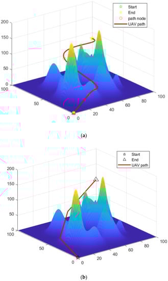
Figure 11.
Results of several algorithms in the same environment: (a) IGA, (b) PRM, (c) IPRM.
Table 2 shows the results obtained by using the IGA, PRM algorithm and IPRM algorithm, respectively, in the same map. The results show that, compared with the IGA algorithm, the IPRM algorithm reduces the track distance by 11.7% and the energy consumption by 16.5%. Compared with the PRM algorithm, the IPRM algorithm reduces the track distance by 4.1% and the energy consumption by 5.9%. The IPRM algorithm is better than the IGA and PRM algorithm in terms of distance and energy consumption.
In order to verify the adaptability of the improved algorithm in different environments, the number of mountains in the environment was changed to 40, the number of sampling points of the IPRM algorithm was set to 20, 40, 60, 80 and 100, respectively, and 10 experiments were conducted. The results are shown in Table 3 and Table 4.
In order to observe the changes in the data in the table more intuitively, a bar chart is shown in Figure 12. It is clear that the IPRM has a significant advantage over PRM in the obtained results.
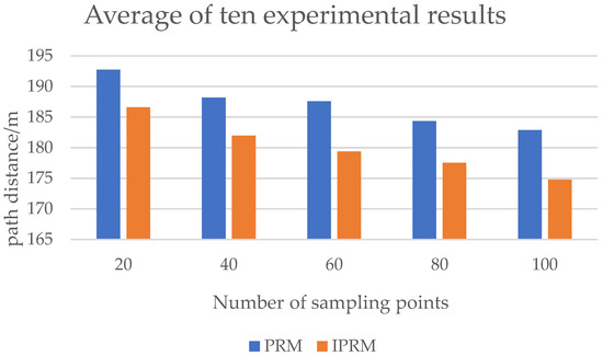
Figure 12.
Results for different number of sampling points.
In Table 3, when the number of sampling point is 20, in the ten experiments of IPRM, there are two cases of no solution. On the one hand, there are too many obstacles near the center in the environment, and, after the optimization of the sampling space, the position of the sampling point is relatively limited. On the other hand, there are few cases of no solution, as shown in Figure 13a,b. When the number of obstacles is reduced, it is obvious that IPRM has more advantages than PRM in generating an undirected road map, and the obtained solution is better, as shown in Figure 13c,d.
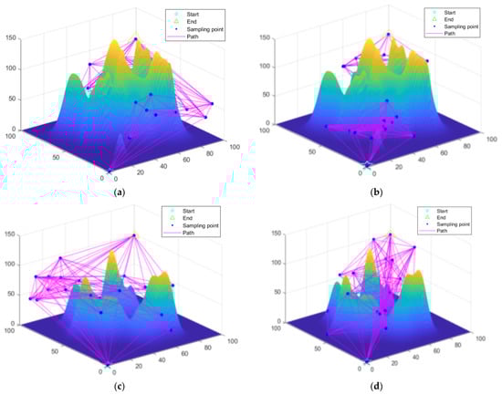
Figure 13.
Planning results under different obstacles: (a) PRM on 40 peaks; (b) IPRM on 40 peaks; (c) PRM on 20 peaks; (d) IPRM on 20 peaks.
In order to verify the impact of the number of obstacles on the results, experiments with a different number of obstacles were tested. When the number of sampling points was 20, the PRM and IPRM were tested 50 times under the number of obstacles of 30, 35 and 40, and the number of unsolved cases was obtained. PRM blue at point 30 is zero, indicating that the solution effect of IPRM is not as good as that of PRM under the influence of an increasing number of obstacles. It can be concluded from Figure 14 that, in the case of a low number of sampling points, the number of multiple obstacles will limit the solution of the IPRM. It also shows that IPRM is more suitable for other situations.
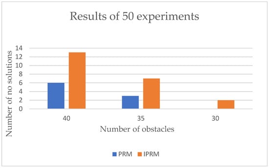
Figure 14.
Results of 50 experiments with different number of obstacles.
In the further improvement of the algorithm, a parameter setting that adaptively adjusts the sampling space can be added. When the algorithm has no solution, the sampling space or the number of sampling points can be appropriately increased until a better solution is found, or an adaptive parameter can be added in order to adjust them properly, decreasing as the distance between the starting point and the ending point decreases, and increasing as the distance between the starting point and the ending point increases. For example, in this paper, the sampling space was an ellipsoid, with the starting point and the end point as the focus. The length of the major axis of the ellipsoid was twice the length of the minor axis, which was a fixed value. We can increase an adaptive value to adjust the multiple. When the distance between the starting point and the end point is long, the multiple will increase appropriately, and when the distance between the starting point and the end point is short, the multiple will decrease appropriately.
6. Conclusions
Aiming at the path planning problem of UAVs with a corner energy consumption model, this paper proposes an improved PRM algorithm. Firstly, in order to simulate the real terrain environment, a mathematical model was established; secondly, an energy consumption model was established; then, the sampling space of the PRM algorithm was optimized to make the obtained path more explicit and improve the utilization rate in space and time; then, the sampling third-order B-spline curve method was used to curve the rotation angle to make the path smoother and the distance shorter. Finally, the IGA, PRM and IPRM were compared through several simulation experiments. Through the analysis of the data results, it can be concluded that the IPRM has significant advantages over other algorithms, mainly in track distance; most importantly, it is superior to other algorithms in terms of energy consumption. In addition, it also has good adaptability in terms of environmental adaptation, but, at the same time, it has a small limitation. When there are too many obstacles, it will limit the algorithm in finding solutions. To sum up, IPRM can be applied to the path planning of UAVs when they are operating in simulated mountains and forests.
Author Contributions
Conceptualization and formal analysis, W.L. and A.Z.; methodology and supervision, L.W.; writing—original draft, W.L. and L.W.; writing—review and editing, W.L. and J.C.; paper layout, L.W.and H.H.; Funding acquisition, L.W. and T.T. All authors have read and agreed to the published version of the manuscript.
Funding
This paper is supported by Anhui Province University Excellent Top Talent Training Project (gxbjZD2022023), the Open Research Fund of Anhui Province Key Laboratory of Detection Technology and Energy Saving Devices, Anhui Polytechnic University (JCKJ2021A06), Anhui Polytechnic University-Jiujiang District Industrial Collaborative Innovation Special Fund Project (2022cyxtb6, 2022cyxtb4), Research Fund Project of Anhui Engineering University (2022YQQ002, Xjky2022002, Xjky2020001), Wuhu science and technology project (Project Leader: Wang Lei).
Institutional Review Board Statement
Not applicable.
Informed Consent Statement
Not applicable.
Data Availability Statement
Not applicable.
Conflicts of Interest
The authors declare no conflict of interest.
References
- Tsouros, D.C.; Bibi, S.; Sarigiannidis, P.G. A review on UAV-based applications for precision agriculture. Information 2019, 10, 349. [Google Scholar] [CrossRef]
- Zhang, Y.K. Flight path planning of agriculture UAV based on improved artificial potential field method. In Proceedings of the 30th Chinese Control and Decision Conference, Shenyang, China, 9–11 June 2018; pp. 1526–1530. [Google Scholar]
- Nikolakopoulos, K.G.; Soura, K.; Koukouvelas, I.K.; Argyropoulosa, N.G. UAV vs. classical aerial photogrammetry for archaeological studies. J. Archaeol. Sci. Rep. 2017, 14, 758–773. [Google Scholar] [CrossRef]
- Pádua, L.; Adão, T.; Hruška, J.; Marques, P.; Sousa, A.; Morais, R.; Lourenco, J.M.; Sousa, J.J.; Peres, E. UAS-based photogrammetry of cultural heritage sites: A case study addressing Chapel of Espírito Santo and photogrammetric software comparison. In Proceedings of the International Conference on Geoinformatics and Data Analysis, Prague, Czechoslovakia, 20–22 April 2018; pp. 72–76. [Google Scholar]
- Calleja, J.F.; Pagés, O.R.; Díaz-Álvarez, N.; Peón, J.; Gutiérrez, N.; Martín-Hernández, E.; Relea, A.C.; Melendi, D.R.; Álvarez, P.F. Detection of buried archaeological remains with the combined use of satellite multispectral data and UAV data. Int. J. Appl. Earth Obs. Geoinf. 2018, 73, 555–573. [Google Scholar] [CrossRef]
- Lipovský, P.; Draganová, K.; Novotňák, J.; Szőke, Z.; Fil’ko, M. Indoor mapping of magnetic fields using UAV equipped with fluxgate magnetometer. Sensors 2021, 21, 4191. [Google Scholar] [CrossRef] [PubMed]
- Mu, Y.; Zhang, X.; Xie, W.; Zheng, Y. Automatic detection of near-surface targets for unmanned aerial vehicle (UAV) magnetic survey. Remote Sens. 2020, 12, 452. [Google Scholar] [CrossRef]
- Aggarwal, S.; Kumar, N. Path planning techniques for unmanned aerial vehicles: A review, solutions, and challenges. Comput. Commun. 2020, 149, 270–299. [Google Scholar] [CrossRef]
- Kumar, A.; Pant, S.; Ram, M. System reliability optimization using gray wolf optimizer algorithm. Qual. Reliab. Eng. Int. 2017, 33, 1327–1335. [Google Scholar] [CrossRef]
- Huang, G.; Cai, Y.; Liu, J.; Qi, Y.; Liu, X. A novel hybrid discrete grey wolf optimizer algorithm for multi-UAV path planning. J. Intell. Robot. Syst. 2021, 103, 49. [Google Scholar] [CrossRef]
- Zhang, S.; Pu, J.; Si, Y.; Sun, L. Path planning for mobile robot using an enhanced ant colony optimization and path geometric optimization. Int. J. Adv. Robot. Syst. 2021, 18, 1–15. [Google Scholar] [CrossRef]
- Wang, W.; Zhao, J.; Li, Z.; Huang, J. Smooth path planning of mobile robot based on improved ant colony algorithm. J. Robot. 2021, 2021, 4109821. [Google Scholar] [CrossRef]
- Zhou, Z.; Wang, J.; Zhu, Z.; Yang, D.; Wu, J. Tangent navigated robot path planning strategy using particle swarm optimized artificial potential field. Optik 2018, 158, 639–651. [Google Scholar] [CrossRef]
- Fu, Y.; Ding, M.; Zhou, C. Phase angle-encoded and quantum-behaved particle swarm optimization applied to three-dimensional route planning for UAV. IEEE Trans. Syst. Man Cybern. -Part A: Syst. Hum. 2011, 42, 511–526. [Google Scholar] [CrossRef]
- Fransen, K.; Eekelen, J. Efficient path planning for automated guided vehicles using A* algorithm incorporating turning costs in search heuristic. Int. J. Prod. Res. 2021, 1–19. [Google Scholar] [CrossRef]
- Tang, G.; Tang, C.; Claramunt, C.; Hu, X.; Zhou, P. Geometric a-star algorithm: An improved a-star algorithm for AGV path planning in a port environment. IEEE Access 2021, 99, 59196–59210. [Google Scholar] [CrossRef]
- Kang, J.G.; Lim, D.W.; Choi, Y.S.; Jang, W.J.; Jung, J.W. Improved RRT-connect algorithm based on triangular inequality for robot path planning. Sensors 2021, 21, 333. [Google Scholar] [CrossRef] [PubMed]
- Zhai, L.; Feng, S. A novel evacuation path planning method based on improved genetic algorithm. J. Intell. Fuzzy Syst. 2022, 42, 1813–1823. [Google Scholar] [CrossRef]
- Lee, J.; Kim, D.W. An effective initialization method for genetic algorithm-based robot path planning using a directed acyclic graph. Inf. Sci. 2016, 332, 1–18. [Google Scholar] [CrossRef]
- Yu, X.; Li, C.; Zhou, J.F. A constrained differential evolution algorithm to solve UAV path planning in disaster scenarios. Knowl. -Based Syst. 2020, 204, 106209. [Google Scholar] [CrossRef]
- Sanchez-Aguero, V.; Valera, F.; Vidal, I.; Tipantuña, C.; Hesselbach, X. Energy-aware management in multi-UAV deployments: Modelling and strategies. Sensors 2020, 20, 2791. [Google Scholar] [CrossRef]
- Li, J.; Lu, D.; Zhang, G.; Tian, J.; Pang, Y. Post-disaster unmanned aerial vehicle base station deployment method based on artificial bee colony algorithm. IEEE Access 2019, 7, 168327–168336. [Google Scholar] [CrossRef]
- Wu, X.; Yin, Y.; Xu, L.; Wu, X.; Meng, F.; Zhen, R. Multi-UAV task allocation based on improved genetic algorithm. IEEE Access 2021, 9, 100369–100379. [Google Scholar] [CrossRef]
- Palossi, D.; Furci, M.; Naldi, R.; Maronggui, A.; Marconi, L.; Benini, L. An energy-efficient parallel algorithm for real-time near-optimal uav path planning. In Proceedings of the ACM International Conference on Computing Frontiers, Como, Italy, 16–18 May 2016; pp. 392–397. [Google Scholar] [CrossRef]
- Cekmez, U.; Ozsiginan, M.; Sahingoz, O.K. A UAV path planning with parallel ACO algorithm on CUDA platform. In Proceedings of the 2014 International Conference on Unmanned Aircraft Systems, Orlando, FL, USA, 27–30 May 2014; pp. 347–354. [Google Scholar] [CrossRef]
- Kavraki, L.E.; Svestka, P.; Latombe, J.C.; Overmars, M.H. Probabilistic roadmaps for path planning in high-dimensional configuration spaces. IEEE Trans. Robot. Autom. 1996, 12, 566–580. [Google Scholar] [CrossRef]
- Gasparetto, A.; Boscariol, P.; Lanzutti, A.; Vidoni, R. Path planning and trajectory planning algorithms: A general overview. Mech. Mach. Sci. 2015, 29, 3–27. [Google Scholar] [CrossRef]
- Tan, J.; Xiao, Y.; Liu, L.; Sun, J. Improved PRM algorithm for path planning of UAV. Transducer Microsyst. Technol. 2020, 39, 38–41. [Google Scholar] [CrossRef]
- Santiago, R.M.C.; Ocampo, A.L.; Ubando, A.T.; Bandala, A.A.; Dadios, E.P. Path planning for mobile robots using genetic algorithm and probabilistic roadmap. In Proceedings of the 9th International Conference on Humanoid, Nanotechnology, Information Technology, Communication and Control, Environment and Management, Manila, Philippines, 29–30 November 2017; pp. 1–5. [Google Scholar] [CrossRef]
- Rantanen, M.T. A connectivity-based method for enhancing sampling in probabilistic roadmap planners. J. Intell. Robot. Syst. 2011, 64, 161–178. [Google Scholar] [CrossRef]
- Boor, V.; Overmars, M.H.; Van Der Stappen, A.F. The Gaussian sampling strategy for probabilistic roadmap planners. In Proceedings of the 1999 IEEE International Conference on Robotics and Automation, Detroit, MI, USA, 10–15 May 1999; pp. 1018–1023. [Google Scholar] [CrossRef]
- Chen, G.; Luo, N.; Liu, D.; Zhao, Z.; Liang, C. Path planning for manipulators based on an improved probabilistic roadmap method. Robot. Comput. -Integr. Manuf. 2021, 72, 102196. [Google Scholar] [CrossRef]
- Foo, J.L.; Knutzon, J.; Kalivarapu, V.; Oliver, J.; Winer, E. Path planning of unmanned aerial vehicles using B-splines and particle swarm optimization. J. Aerosp. Comput. Inf. Commun. 2009, 6, 271–290. [Google Scholar] [CrossRef]
- Cao, K.; Cheng, Q.; Gao, S.; Chen, Y.Q.; Chen, C.B. Improved PRM for path planning in narrow passages. In Proceedings of the 2019 IEEE International Conference on Mechatronics and Automation (ICMA), Tianjin, China, 4–7 August 2019; pp. 45–50. [Google Scholar]
- Huang, S.; Tian, J.; Qiao, L.; Wang, Q.; Su, Y. Unmanned aerial vehicle path planning based on improved genetic algorithm. J. Comput. Appl. 2021, 41, 390–397. [Google Scholar] [CrossRef]


Publisher’s Note: MDPI stays neutral with regard to jurisdictional claims in published maps and institutional affiliations. |
© 2022 by the authors. Licensee MDPI, Basel, Switzerland. This article is an open access article distributed under the terms and conditions of the Creative Commons Attribution (CC BY) license (https://creativecommons.org/licenses/by/4.0/).