Equilibrium Optimization with Multi-Energy-Efficiency-Grade Products: Government and Market Perspective

Abstract

This paper studies the multi-level supply chain network equilibrium optimization problem of multi-energy-efficiency products under different government subsidies and demand scales. In the equilibrium optimization problem, manufacturers determine the production volume of the energy-saving products; retailers decide the transaction volume with manufacturers, distribution volume for markets, and marketing efforts of energy-saving products; markets determine the transaction price. Firstly, the optimal decision-making behaviors of manufacturers, retailers, and markets are described. Simultaneously, the global optimization problem is transformed into a finite-dimensional variational inequality formulation. Then, the equilibrium conditions of the whole supply chain network are derived by the Euler method. Finally, a case study verifies the effectiveness of the proposed method. Interestingly, we found that energy-saving subsidies and demand scales were negatively correlated with the marketing efforts of the subsidized retailers for high energy-efficient products and positively correlated with the marketing efforts of non-subsidized retailers for high energy-efficient products in the same market; the development of retailers in the same market tended to be consistent, and the differentiation of the demand scale eliminated the retailers without a competitive advantage.

1. Introduction

The problem of energy shortage restricts the economic and social development of many developing countries, including China, Mexico, and India, to name a few [1]. Since the beginning of the 21st century, improving energy efficiency has become China’s main energy policy goal. Between 2000 and 2008, the share of household energy demand in total energy consumption rose from 7% to 11%. Over the same period, residential electricity consumption tripled. To a large extent, this is driven by the increase of household appliances. Therefore, spreading and using energy-saving products can reduce the energy pressure throughout the world. As we all know, energy-saving products significantly impact energy and the economy only after consumers widely accept them. Therefore, the government has repeatedly subsidized consumers to increase the energy-saving products’ demand [2]. For example, in 2007, when consumers bought energy-saving appliances of level 2 or above (There are five energy-saving ranks in total, and level 2 or above means a high energy-saving product.) in China, they could get a government subsidy as a rebate equivalent to 13% of the price [3]; in 2012, China launched a 26.5-billion-yuan subsidy program for energy-saving household appliances, giving consumers 5% to 10% price concessions [4]; in 2019, Beijing implemented a new energy-saving subsidy policy, in which consumers who purchase primary energy-efficient products from designated retailers receive a subsidy equivalent to 13% of the product price and 8% of the 2-level energy-saving appliances (http://www.beijing.gov.cn/zhengce/gfxwj/sj/201905/t20190522_61828.html, accessed on 10 June 2021). Besides, similar subsidy policies have also been widely implemented in many industries around the world. For example, in the United States, consumers can receive government tax incentives when they buy new energy vehicles [5]; in Norway and the Netherlands, consumers who purchase energy-efficient products can receive tax credits [4,6].

An effective subsidy policy can standardize the economic behavior of market entities, improve social benefits, and achieve the government’s macro-control and strategic development goals. How to make a subsidy policy is a vital topic. Many scholars have studied it with a single enterprise. However, in practice, no enterprise can exist independently. The decisions of subsidized enterprises are not only affected by government subsidies, but also interact with other enterprises’ decisions. Therefore, this paper studied the optimal decision-making problem of supply chain network (SCN) members considering government subsidies and the relationship between multiple manufacturers, retailers, and markets, which is more in line with practice.

Government subsidies can increase the competitiveness of products and benefit consumers [7]. Consumer preference plays a crucial role in the optimal decision-making of SCN members. In this paper, the heterogeneity of consumers’ preferences for retailers is mainly reflected in the demand scales for retailers. In the real world, the influence of retailers’ demand scales is evident in the decision-making process of the supply chain upstream and downstream. Hence, it is necessary to study the impact of energy-saving subsidies on the supply chain network equilibrium (SCNE) from the perspective of demand scales for retailers.

Under the influence of government energy-saving subsidies and customer demand scales, how SCN members make decisions has become a hot topic in recent years. Some scholars have studied the supply chain performance considering the government energy-saving subsidy policy [8,9,10,11]. However, their research object was a single supply chain. The current supply chain system is not a single chain structure but a multi-level network composed of multiple suppliers, manufacturers, transporters, and markets. Besides, the demand scales in different regions are not identical.

When designing the subsidy scheme, the government should consider the financial expenditure and the impact of the subsidy policy on the overall social welfare of the SCN. The main goal of our research was to answer the following two questions: (Q1) how does the energy saving subsidy affect the equilibrium results of decision variables? In addition, we also observed an interesting phenomenon in reality: in Jingdong’s and Gome’s self-owned stores, we found that each store’s recommendation of energy-saving products is different; that is, the marketing efforts are diverse. Hence, the other question is: (Q2) why does this phenomenon appear?

This study simultaneously establishes the SCNE model with multi-energy-efficiency-grade products considering government energy-saving subsidies and demand scales, which is different from the previous literature on energy-saving subsidies for a single supply chain. In addition, we also innovatively introduce subsidy region and object differentiation into the SCNE model. The model proposed in this paper is practical, and the main contributions are as follows:

(1) Considering the energy-saving subsidy policy, this paper studies the SCNE problem with multi-energy-efficiency-grade products from government and market perspectives. The influences of the internal and external environment on the decision-making of SCN members are obtained simultaneously.

(2) Some scenarios are assumed to provide a more comprehensive reference for formulating energy-saving subsidy policies and enterprises’ decisions in SCN.

(3) This paper explains retailers’ behavior in response to the government’s energy-saving subsidy policy. That is why retailers have different marketing efforts for the same energy-saving product.

This rest of the paper is organized as follows: The literature review is given in Section 2; in Section 3, the equilibrium model of SCN is presented; qualitative properties and the solution method are provided in Section 4; a numerical example is shown in Section 5; an elaborate discussion and a comparative analysis are organized in Section 6; finally, some conclusions and future research direction are summarized in Section 7.

2. Literature Review

This paper mainly focuses on how SCN members make decisions considering energy-saving subsidy policies and demand scales. The existing research review is divided into three branches: energy-saving subsidy policy, marketing efforts, and SCNE.

2.1. Energy-Saving Subsidy Policy

Research has confirmed that household appliances were the main factor in household energy consumption [12]. Improving consumers’ willingness to buy energy-saving appliances was necessary to achieve energy conservation. Since the end of 2016, the Chinese government has promulgated more than 30 policies, and local governments have published more than 700 environmental laws and regulations to save resources. It has become a fact that energy-saving subsidies can stimulate consumers to buy energy-saving products. Yi and Li [8] believe that subsidy policies can achieve energy conservation and emission reduction, while carbon tax policies are not always the same. Zhang et al. [13] studied the reuse of energy-saving products and analyzed the impact of different subsidy policies on supply chain members’ decision-making. Krass et al. [14] studied the effect of subsidies on firms’ adoption of cleaner production technologies, and the results showed that subsidies were usually beneficial. Bi et al. [15] studied how the government implements a subsidy policy to encourage enterprises to adopt green emission reduction technology. Madani and Rasti-Barzoki [16] concluded that the effect of subsidies on profits and sustainability is greater than that of taxes. The above research was primarily interested in a single supply chain, without considering the interaction between supply chains, a more common phenomenon in the real world.

2.2. Marketing Efforts

Marketing efforts are a common way for retailers to stimulate market demand and increase sales revenue. Regarding supply-chain decision-making, Taylor [17] pointed out that retailers would put in the optimal marketing efforts to achieve channel coordination when marketing efforts affected demand. Considering product quality and sales efforts, Song et al. [18] analyzed the influence of different channel power structures on manufacturers and retailers. Ma et al. [19] explored the importance of marketing efforts on supply chain decisions under symmetric and asymmetric information. Li et al. [20] established a two-stage non-cooperative game model and analyzed the influence of advertising parameters on members’ decision-making in a closed-loop supply chain. Sarkar et al. [21] defined the basic costs, such as sales price and advertising cost, as fuzzy driving and analyzed the impact of marketing efforts on the overall supply chain revenue under uncertainty. Generally speaking, the research on the effects of marketing efforts on a single supply chain is rich. However, the environment of manufacturers, retailers, and markets is currently more complex. Only considering the relationship between the upstream and downstream of a single supply chain is not appropriate.

2.3. Supply Chain Network Equilibrium

SCN is a complex system with a network structure formed by cross-business supply chain enterprises. Nagurney [22] constructed a three-tier SCNE model composed of manufacturers, retailers, and markets and studied the optimal behavior of SCN members for the first time. Then, the generalized Nash equilibrium theory was used to analyze multi-members and multi-products [23,24]. During this period, some scholars extended Nagurney’s model [19,25,26,27,28,29]. Besides, some researchers paid more attention to the design of SCN [30,31,32,33]. Through the above research, we found that scholars have produced much research on SCN. However, we studied the equilibrium optimization of SCNE from the perspective of government and the market, which is different from previous research. This paper provides a new view of the study of SCNE.

3. Materials and Methods

Manufacturers, retailers, and market optimization models were established with an energy-saving subsidy policy. Then, according to the variational inequality theory, the SCN’s equilibrium condition was obtained.

3.1. Problem Definition

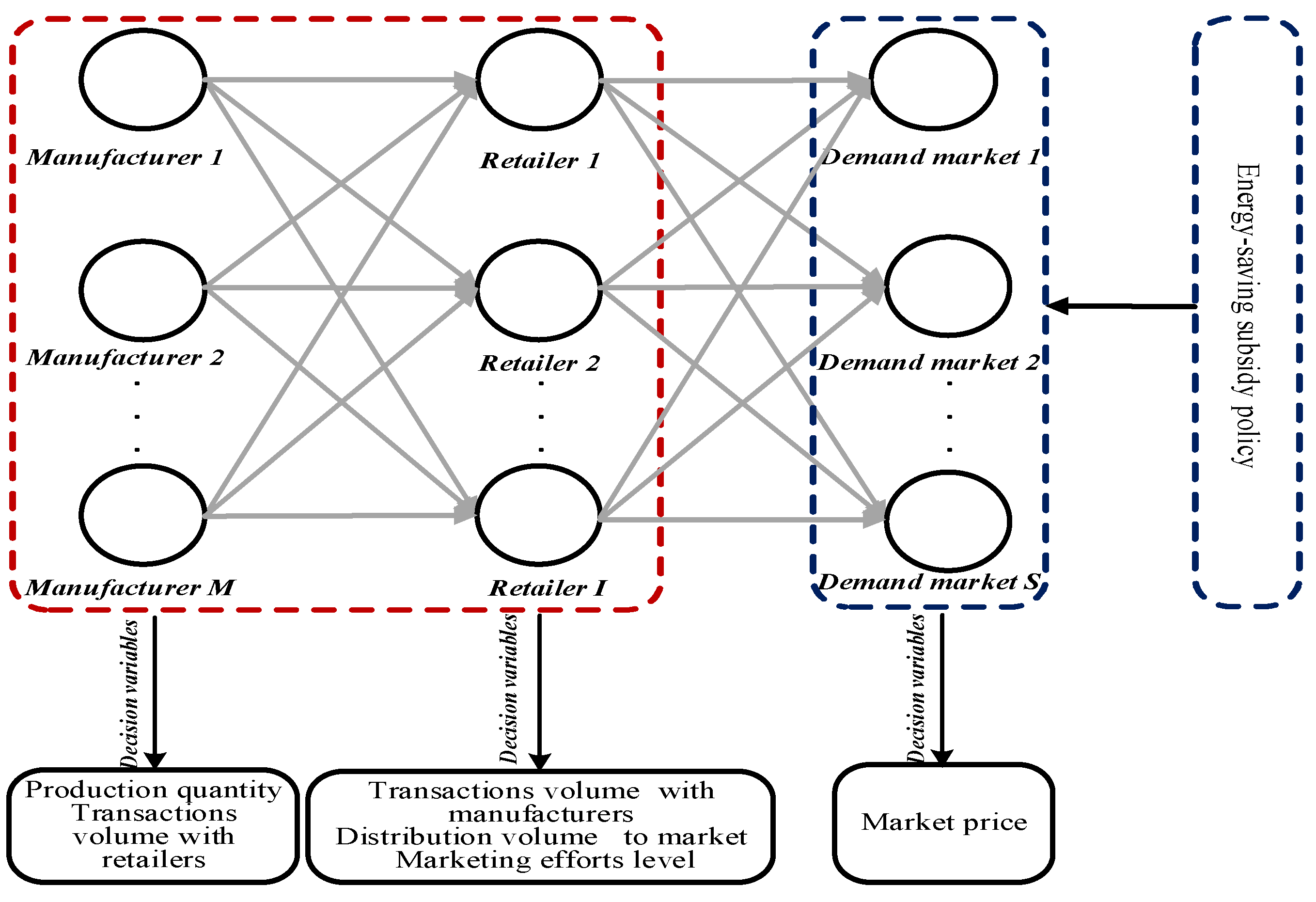
This paper constructs a three-tier SCNE model consisting of multiple manufacturers, retailers, and markets. In Figure 1, the retailer i orders products from the manufacturer m and sells them to the markets. The gray arrow indicates the direction of the flow of multi-energy-efficiency-grade products. In addition, the manufacturer’s decision variables are product yield and transaction volume with retailers; the decision variables of retailers are the transaction volume with manufacturers, the distribution quantity to market, and the marketing effort for multi-energy-efficiency-grade products; the decision variable of markets is the transaction price. The description of relevant symbols in the model is shown in

Table 1. Symbol description.

Symbol		Description
Set	M	A set of all manufacturers in SCN, where $m\in M$
	I	A set of all retailers in SCN, where $i\in I$
	S	A set of all markets in SCN, where $s\in S$
	N	A set of all products’ energy-efficiency-grade, where $n\in N$
Decision variables	$q_m^n$	The quantity of n energy-efficiency-grade products (n-EEGP) produced by manufacturer m
	$q_{mi}^n$	The transaction quantity of n-EEGP between manufacturer m and retailer i
	$q_{is}^n$	The distribution quantity of n-EEGP between retailer i and market s
	$p_{si}^n$	The transaction price that consumers in market s pay for n-EEGP of retailer i.
	$u_i^n$	Retailer i’s marketing investment in n-EEGP
Parameter	$G_{si}^n$	Energy-saving subsidy rate when the customer of market s purchase unit n-EEGP in retailer i
	$v_{si}^n$	Demand scales of market s for retailer i’s n-EEGP
	co	Unit-shortage cost of retailer i
	cu	Unit-inventory cost of retailer i
Function	$V{C}_m^n(q_m^n)$	The product cost function of n-EEGP of manufacturer m
	$T{C}_{mi}^n(q_{mi}^n)$	Transaction cost function of n-EEGP between manufacturer m and retailer i
	$H{C}_{mi}^n(q_{mi}^n)$	The handle cost function of retailer i handles n-EEGP from manufacturer m
	$H{C}_{si}^n(q_{si}^n)$	The handle cost function of retailer i handles n-EEGP to market s
	$M{F}_i^n(u_i^n,q_{si}^n)$	Retailer i’s marketing efforts for n-EEGP
	$D_{si}^n(p_{si}^n,u_i^n)$	Market s’s demand for n-EEGP at retailer i

. A roadmap (Figure 2) is presented to help readers understand what follows and the related methods by which the problems are modeled or solved.

3.2. The Optimality Conditions of Manufacturers

Competitive manufacturers produce different energy-efficiency-grade products in a non-cooperative way and sell them to retailers. The manufacturer’s decision variable is $q_{mi}^n$, which represents the transaction quantity between manufacturer m and retailer i. ${\widehat{Q}}_i^n={\left(q_{1i}^n,q_{2i}^n,\dots ,q_{mi}^n\right)}^T$ is the vector of transactions quantity of n-EEGP between all manufacturers and retailer i. ${\widehat{Q}}_i={\left({\widehat{Q}}_i^1,{\widehat{Q}}_i^2,\dots ,{\widehat{Q}}_i^n\right)}^T$ is the vector of transactions quantity of all products between all manufacturers and retailer i. $\widehat{Q}={\left({\widehat{Q}}_1,{\widehat{Q}}_2,\dots ,{\widehat{Q}}_i\right)}^T$ is the vector of transactions quantity of all products between all manufacturers and all retailers. Then, the profit of the manufacturer m is equal to the income minus the production cost $V{C}_m^n(q_m^n)$ and the transaction cost ${\displaystyle \sum _{i=1}^{I}T{C}_{mi}^n(q_{mi}^n)}$. The profit maximization model of manufacturer m is as follows:

$$\max {\pi }_m={\displaystyle \sum _{n=1}^N\left({\displaystyle \sum _{i=1}^I{q}_{mi}^n}{p}_{mi}^n-{\displaystyle \sum _{i=1}^{I}T{C}_{mi}^n(q_{mi}^n)}-V{C}_m^n(q_m^n)\right)}$$

(1)

s.t.

$${\displaystyle \sum _{i=1}^I{q}_{mi}^n}=q_m^n$$

(2)

$q_{mi}^n\ge 0$ for all m, i, n.

Constraint (2) indicates that the quantity of n-EEGP produced by manufacturer m equals the sum of the transaction volume of n-EEGP between manufacturer m and retailer i. Assuming the production and transaction cost function of manufacturer m are continuous differentiable convex functions. The optimality conditions of all manufacturers can be obtained by solving variational inequalities (VI) (3) [34]. That is, determine $Q^{*}\in R_{+}^{MIN}$ such that

$${\displaystyle \sum _{n=1}^N{\displaystyle \sum _{m=1}^M{\displaystyle \sum _{i=1}^I\left[\frac{\partial V{C}_m^n(q_m^{*n})}{\partial q_{mi}^{*n}}+{\displaystyle \sum _{i=1}^I\frac{\partial T{C}_{mi}^n(q_{mi}^{*n})}{\partial q_{mi}^{*n}}}-p_{mi}^n\right]\times \left[q_{mi}^n-q_{mi}^{*n}\right]\ge 0,\hspace{0.17em}}}}\forall Q^{*}\in R_{+}^{MIN}$$

(3)

According to the equivalence of the variational inequality and complementarity problem (the variables are nonnegative), VI (3) satisfies Condition (4).

$$\{\begin{array}{l}\left(\frac{\partial V{C}_m^n(q_m^{*n})}{\partial q_m^n}+{\displaystyle \sum _{i=1}^I\frac{\partial T{C}_{mi}^n(q_{mi}^{*n})}{\partial q_{mi}^n}}-p_{mi}^n\right)\times q_{mi}^{*n}=0\\ q_{mi}^{*n}\ge 0\\ \frac{\partial V{C}_m^n(q_m^{*n})}{\partial q_m^n}+{\displaystyle \sum _{i=1}^I\frac{\partial T{C}_{mi}^n(q_{mi}^{*n})}{\partial q_{mi}^n}}-p_{mi}^n\ge 0\end{array}$$

(4)

where $n=1,2,\dots ,N$; $m=1,2,\dots ,M$; $i=1,2,\dots ,I$.

Condition (4) has an economic significance: in the equilibrium state, if the transaction price is equal to the sum of marginal production cost and transaction cost, then the transaction behavior of n-EEGP will occur between manufacturer m and retailer i. That is, $q_{mi}^n>0$. Otherwise, the transaction behavior of n-EEGP will not occur. That is, $q_{mi}^n=0$. Therefore, when the transaction behavior of n-EEGP occurs, the transaction price of the manufacturer m is equal to $\frac{\partial V{C}_m^n(q_m^{*n})}{\partial q_m^n}+{\displaystyle \sum _{i=1}^I\frac{\partial T{C}_{mi}^n(q_{mi}^{*n})}{\partial q_{mi}^n}}$.

3.3. The Optimality Conditions of Retailers

With the aggravation of economic globalization competition, demand scales are continually changing. The rapid development of products and the increasing flexibility of manufacturing systems not only bring benefits to consumers but also exacerbate the uncertainty of market demand, making it very difficult for retailers in SCN to make order plans. This paper assumes that demand scales are random in an environment of great uncertainty and fluctuation [35].

$D_{si}^n(p_{si}^n,u_i^n)$ represents the demand of market s for retailer i, where $D_{si}^n(p_{si}^n,u_i^n)$ obeys probability density function $f_{si}^n(x;p_{si}^n,u_i^n)$ and probability distribution function $F_{si}^n(x;p_{si}^n,u_i^n)$. Assume that stochastic demand’s cumulative distribution function $D_{si}^n(p_{si}^n,u_i^n)$ is continuous, differentiable, reversible, and strictly increasing, where $F_{si}^n(x;p_{si}^n,u_i^n)={\displaystyle {\int }_0^x{f}_{si}^n(x;p_{si}^n,u_i^n)}dx$. Suppose the retailer’s unit-inventory cost is $c_o$; the retailer’s unit out-of-stock cost is $c_u$. $c_u$ and $c_o$ are all positive numbers. The transaction price between retailer i and manufacturer m is $p_{mi}^n$; the transaction price between retailer i and market s is $p_{si}^n$.

Then, the transaction quantity of retailer i and market s can be expressed as $\min \left\{q_{si}^n,D_{si}^n(p_{si}^n,u_i^n)\right\}$. The out-of-stock quantity of retailer i can be defined as $\max \left\{D_{si}^n(p_{si}^n,u_i^n)-q_{si}^n,0\right\}$. The inventory quantity of retailer i can be described as $\max \left\{q_{si}^n-D_{si}^n(p_{si}^n,u_i^n),0\right\}$.

The retailer’s profit can be expressed as: sales revenue minus purchase cost, handle cost, inventory cost, out-of-stock cost, and marketing efforts’ cost. The profit maximization model of retailer i is as follows:

$$\max {\pi }_i={\displaystyle \sum _{n=1}^N\left(\begin{array}{l}{\displaystyle \sum _{s=1}^S\min \left\{q_{si}^n,D_{si}^n(p_{si}^n,u_i^n)\right\}{p}_{si}^n\left(1+G_{si}^n\right)}\\ -{\displaystyle \sum _{m=1}^{M}H{C}_{mi}^n(q_{mi}^n)}-{\displaystyle \sum _{s=1}^{S}H{C}_{si}^n(q_{si}^n)}\\ -{\displaystyle \sum _{s=1}^S{c}_u\max \left\{0,D_{si}^n(p_{si}^n,u_i^n)-q_{si}^n\right\}}\\ -{\displaystyle \sum _{s=1}^S{c}_o\max \left\{0,q_{si}^n-D_{si}^n(p_{si}^n,u_i^n)\right\}}\\ -{\displaystyle \sum _{m=1}^M{q}_{mi}^n{p}_{mi}^n}-M{F}_i^n\left(u_i^n,q_{si}^n\right)\end{array}\right)}$$

(5)

s.t.

$${\displaystyle \sum _{s=1}^S{q}_{si}^n}={\displaystyle \sum _{m=1}^M{q}_{mi}^n}, q_{mi}^n,q_{si}^n\ge 0 \mathrm{for} \mathrm{all} m, i, s, n$$

(6)

where, ${\pi }_i$ represents the profit of retailer i. $\lambda$ is the cost coefficient of marketing efforts and market efforts cost is $M{F}_i^n(u_i^n,q_{si}^n)=\frac{1}{2}{u}_i^n{}^2{\displaystyle \sum _{s=1}^S{q}_{si}^n}$. Then, equality constraint (6) is transformed into inequality (7) and inequality (8):

$${\displaystyle \sum _{s=1}^S{q}_{si}^n}\le {\displaystyle \sum _{m=1}^M{q}_{mi}^n}$$

(7)

$$-{\displaystyle \sum _{s=1}^S{q}_{si}^n}\ge -{\displaystyle \sum _{m=1}^M{q}_{mi}^n}$$

(8)

Because the market demand is uncertain, then ${\pi }_i$‘s expectation is $E\left({\pi }_i\right)$

$$\max E\left({\pi }_i\right)={\displaystyle \sum _{n=1}^N\left[\begin{array}{l}{\displaystyle \sum _{s=1}^S{\displaystyle {\int }_0^{q_{si}^n}\left(\begin{array}{l}{p}_{si}^n\left(1+G_{si}^n\right)x\\ -c_o(q_{si}^n-x)\end{array}\right)f_{si}^n(x;p_{si}^n,u_i^n)dx}}\\ +{\displaystyle \sum _{s=1}^S{\displaystyle {\int }_{q_{si}^n}^{+\infty }\left(\begin{array}{l}{p}_{si}^n\left(1+G_{si}^n\right)q_{si}^n\\ -c_u(x-q_{si}^n)\end{array}\right)f_{si}^n(x;p_{si}^n,u_i^n)dx}}\\ -{\displaystyle \sum _{m=1}^{M}H{C}_{mi}^n(q_{mi}^n)}-{\displaystyle \sum _{s=1}^{S}H{C}_{si}^n(q_{si}^n)}\\ -{\displaystyle \sum _{m=1}^M{p}_{mi}^n{q}_{mi}^n}-M{F}_i^n\left(u_i^n,q_{si}^n\right)\end{array}\right]}$$

(9)

Theorem 1. 

$\min E\left({\pi }_i\right)$ is a concave function of the transaction quantity $q_{mi}^n$ and the distribution quantity $q_{si}^n$.

Proof.

Proof of Theorem 1 is shown in Appendix A.

According to Theorem 1, there are optimal $q_{mi}^n$ and $q_{si}^n$ to maximize $E\left({\pi }_i\right)$.

Assuming that ${\theta }_1^{}=\left({\theta }_{11},{\theta }_{21},\dots ,{\theta }_{i1}\right)$ and ${\theta }_2^{}=\left({\theta }_{12},{\theta }_{22},\dots ,{\theta }_{i2}\right)$ are Lagrange multipliers of constraints (7) and (8), where ${\theta }_{i1}=\left({\theta }_{i1}^1,{\theta }_{i1}^2,\dots ,{\theta }_{i1}^N\right)$ and ${\theta }_{i2}^{}=\left({\theta }_{i2}^1,{\theta }_{i2}^2,\dots ,{\theta }_{i2}^N\right)$. ${\tilde{Q}}_i^n={\left(q_{1i}^n,q_{2i}^n,\dots ,q_{si}^n\right)}^T$ is the n-EEGP’s distribution volume vector of retailer i to all markets. ${\tilde{Q}}_i={\left({\tilde{Q}}_i^1,{\tilde{Q}}_i^2,\dots ,{\tilde{Q}}_i^n\right)}^T$ is the all-products’ distribution volume vector of retailer i to all markets. $\tilde{Q}={\left({\tilde{Q}}_1,{\tilde{Q}}_2,\dots ,{\tilde{Q}}_i\right)}^T$ is the volume vector of all retailers distributing all products to all markets. $U_i^{}={\left(u_i^1,u_i^2,\dots ,u_i^n\right)}^T$ is the marketing efforts of retailer i for all products. $U={\left(U_1,U_2,\dots ,U_i\right)}^T$ represents the marketing efforts of all retailers for all products. All retailers in the SCN compete in a non-cooperative way, then the equilibrium conditions of all retailers’ decisions can be obtained [34]. Determine the equilibrium vector $\left({\tilde{Q}}^{*},U^{*},{\theta }_1^{*},{\theta }_2^{*}\right)\in R_{+}^{MIN+IN+2ISN}$ satisfied VI (10).

$${\displaystyle \sum _{n=1}^N\left(\begin{array}{l}{\displaystyle \sum _{i=1}^I{\displaystyle \sum _{s=1}^S{R}_1\times \left[q_{si}^n-q_{si}^{\ast n}\right]}}+{\displaystyle \sum _{m=1}^M{\displaystyle \sum _{i=1}^I{R}_2\times \left[q_{mi}^n-q_{mi}^{*n}\right]}}\\ +{\displaystyle \sum _{i=1}^I{R}_3\times \left[{\theta }_{i1}^n-{\theta }_{i1}^{*n}\right]}+{\displaystyle \sum _{i=1}^I{R}_4\times \left[{\theta }_{i2}^n-{\theta }_{i2}^{*n}\right]}\\ +{\displaystyle \sum _{i=1}^I{R}_5}\times \left[u_i^n-u_i^{\ast n}\right]\end{array}\right)}\ge 0\hspace{0.17em}$$

(10)

where, $\forall m,i,s,n\hspace{0.17em}\hspace{0.17em}\hspace{0.17em}\left({\tilde{Q}}^{*},U^{*},{\theta }_1^{*},{\theta }_2^{*}\right)\in R_{+}^{MIN+IN+2ISN}$, $R_1$,$R_2$,$R_3$,$R_4$, and $R_5$ in VI (10) are obtained in Abbreviations. □

3.4. The Optimality Conditions of Markets

The market is at the end of SCN. Consumers trade with retailers in the market. For any retailer, when the market is at equilibrium, consumer behavior should satisfy equilibrium conditions (11) [36].

Formula (11) shows the relationship between the supply of retailer i and the demand of market s for retailer i. When the transaction price is 0, it means that supply exceeds demand. When the demand price is greater than 0, the supply of retailer i and demand of market s for retailer i reach equilibrium, where $E\left(D_{si}^n(p_{si}^n,u_i^n)\right)$ indicates the expectation of $D_{si}^n(p_{si}^n,u_i^n)$. Then,

$$E\left(D_{si}^n(p_{si}^{*n},u_i^{*n})\right)\{\begin{array}{c}\le q_{si}^{*n}\hspace{0.17em}\hspace{0.17em}\hspace{0.17em}\hspace{0.17em}if\hspace{0.17em}{p}_{si}^{*n}=0\hspace{0.17em}\hspace{0.17em}\forall \hspace{0.17em}i,s,n\\ =q_{si}^{*n}\hspace{0.17em}\hspace{0.17em}\hspace{0.17em}\hspace{0.17em}if\hspace{0.17em}{p}_{si}^{*n}>0\hspace{0.17em}\hspace{0.17em}\forall \hspace{0.17em}\hspace{0.17em}i,s,n\end{array}$$

(11)

Formula (11) indicates that if the transaction price between the retailer and the market is 0, then the retailer’s supply is greater than the market demand; if the transaction price between the retailer and the market is greater than 0, then the retailer’s supply is equal to the market demand. $P_i^n={\left(p_{1i}^n,p_{2i}^n,\dots ,p_{si}^n\right)}^T$ is the n-EEGP’s transaction price vector of retailer i and all markets. $P_i={\left(P_i^1,P_i^2,\dots ,P_i^n\right)}^T$ is the transaction price vector of all products between retailer i and all markets. $P={\left(P_1,P_2,\dots ,P_i\right)}^T$ is the transaction price vector all products between all retailers and all markets. According to the relationship between equilibrium optimization and variational inequality problem, the optimal behavior of market layer can be expressed in VI (12). That is determine $P^{*}\in R_{+}^{SIN}$ to satisfy VI (12).

$${\displaystyle \sum _{n=1}^N{\displaystyle \sum _{i=1}^I{\displaystyle \sum _{s=1}^S\left[q_{is}^{*n}-D_{si}^n(p_{si}^{*n},u_i^{*n})\right]\times \left[p_{si}^n-p_{si}^{*n}\right]}}}\ge 0$$

(12)

3.5. The Optimality Conditions of Supply Chain Network

When SCN reaches equilibrium, the optimal solution of the manufacturer satisfies the VI (3), the retailer satisfies the VI (10), and the market meets the VI (12). The sum of VI (3), VI (10), and VI (12) is satisfied by the product production of the manufacturer, the transaction volume between manufacturers and retailers, the distribution quality between the retailer and the market, and the transaction price. According to the relevant theories in research, the definition of SCNE is given [22,37].

Definition 1. 

The transaction volume between manufacturers and retailers, retailer’s distribution volume to markets, transaction price between retailers and markets, retailer’s marketing effort for products and Lagrange multipliers $\left({\widehat{Q}}^{*},{\tilde{Q}}^{*},P^{*},U^{*},{\theta }_1^{*},{\theta }_2^{*}\right)\in k$ is the equilibrium solution of SCN considering energy-saving subsidy policy if it can make VI (3), VI (10), and VI (12) nonnegative.

Theorem 2. 

$\left(Q^{*},{\tilde{Q}}^{*},P^{*},U^{*},{\theta }_1^{*},{\theta }_2^{*}\right)\in k$ satisfies the VI (13), then, $\left(Q^{*},{\tilde{Q}}^{*},P^{*},U^{*},{\theta }_1^{*},{\theta }_2^{*}\right)\in k$ is the equilibrium condition of SCN considering the government subsidy and demand scale according to Definition 1.

$${\displaystyle \sum _{n=1}^N\left(\begin{array}{l}{\displaystyle \sum _{m=1}^M{\displaystyle \sum _{i=1}^I{W}_1\times \left[q_{mi}^n-q_{mi}^{*n}\right]}}+{\displaystyle \sum _{i=1}^I{\displaystyle \sum _{s=1}^S{W}_2\times \left[q_{si}^n-q_{si}^{\ast n}\right]}}\\ +{\displaystyle \sum _{i=1}^I{\displaystyle \sum _{s=1}^S{W}_3\times \left[p_{si}^n-p_{si}^{*n}\right]}}+{\displaystyle \sum _{i=1}^I{R}_3\times \left[{\theta }_{i1}^n-{\theta }_{i1}^{*n}\right]}\\ +{\displaystyle \sum _{i=1}^I{R}_4\times \left[{\theta }_{i2}^n-{\theta }_{i2}^{*n}\right]}+{\displaystyle \sum _{i=1}^I{W}_4}\times \left[u_i^n-u_i^{\ast n}\right]\end{array}\right)}\ge 0\hspace{0.17em}$$

(13)

where $W_1$,$W_2$,$W_3$, and $W_4$, in VI (13) are obtained in Abbreviations.

Proof. 

Proof of Theorem 2 is presented in Appendix A. □

4. Qualitative Property and Solution Method

4.1. Qualitative Property

This section proves the existence and uniqueness of the solution of VI (13). The solution of VI (13) refers to the SCN’s equilibrium solution considering government subsidy policy and marketing efforts.

Since the feasible set of VI (13) is not a compact set, we cannot merely conclude that VI (13) exists from function continuity. A weak condition to ensure the existence of the solution is needed. Let $k=\{\left(Q^{*},{\tilde{Q}}^{*},P^{*},U^{*},{\theta }_1^{*},{\theta }_2^{*}\right)|0\le \widehat{Q}\le \overline{\widehat{Q}},0\le \tilde{Q}\le \overline{\tilde{Q}},0\le P\le \overline{P},0\le U\le \overline{U}$$,0\le {\theta }_1\le {\overline{\theta }}_1,0\le {\theta }_2\le {\overline{\theta }}_2\}$. Then, $\left({\widehat{Q}}^{*},{\tilde{Q}}^{*},P^{*},U^{*},{\theta }_1^{*},{\theta }_2^{*}\right)\in k$ equals $q_{mi}^n\le \overline{\widehat{Q}},q_{si}^n\le \overline{\tilde{Q}}$$,p_{si}^n\le \overline{P},u_i^n\le \overline{U}{\theta }_{i1}^n\le {\overline{\theta }}_1,{\theta }_{i2}^n\le {\overline{\theta }}_2\hspace{0.17em}\forall n,m,i,s$. That is, k is a closed convex subset of $R^{NMI+2NSI+NI+NI1+NI2}$. Because k is compact and F is continuous, the VI (14) has at least one solution $X\in k$.

$$\langle F(X^{*}),X-X^{*}\rangle \ge 0,\hspace{0.17em}\forall X\in k$$

(14)

Theorem 3.

(Uniqueness). Suppose the cost function $V{C}_m^n(q_m^n)$, $T{C}_{mi}^n(q_{mi}^n)$, $H{C}_{mi}^n(q_{mi}^n)$, and $H{C}_{si}^n(q_{si}^n)$ are convex for $\forall N,\forall M,\forall I,\forall S$, and $p_{si}^n$ is the monotone decreasing function of $E\left(D_{is}^n(p_{si}^n,u_i^n)\right)$. Then VI (13) has a unique solution.

Proof.

Proof of Theorem 3 is presented in Appendix A. □

4.2. Solution Method

The common algorithms for solving SCNE model are the Euler method and the modified projection algorithm. In this paper, the Euler method is used to solve the variational inequality. Compared with the modified projection algorithm, each iteration of the Euler algorithm is more straightforward. The main steps of the algorithm are as follows [37,38].

Step 1: Initialization. Set $u^0\in \Omega ,\alpha$ and $\epsilon$.

Step 2: Computation. Solve the following convex quadratic programming problem at iteration t:

$$u^{t+1}=\arg \min \frac{1}{2}{u}^{T}u-{(u^t+\alpha F(u^t))}^{t}u$$

Step 3: Convergence verification. If $\Vert u^{t+1}-u^t\Vert \le \epsilon$, then stop; otherwise, set $t=t+1$, and go to Step 2.

5. Numerical Example

In this section, some examples are given to illustrate how the energy-saving subsidy policy affects the decision-making of SCN members. Assume that there are two manufacturers, two retailers, and two markets. Retailers order high energy-efficient products (HEEP) and low energy-efficient products (LEEP) from manufacturers and sell them to demand markets. We used the Euler method to solve the model, the iteration step was 0.001, and and the convergence parameter was set to 2 × 10⁻⁶. It was mainly used to solve the following problems in Figure 3 and give corresponding management insights for the members of SCN.

The demand scales for HEEP and LEEP were divided into some scenarios:

Firstly, assuming consumers have the same or different demand scales for HEEP and LEEP, we explored the impact of the energy-saving subsidy policy on SCN results in three cases: ① the government subsidizes all HEEP. ② the government only subsidizes HEEP in market 1. ③ the government subsidizes the HEEP of retailer 1 in market 1.

Then, the above scenarios were divided into two categories: whether there are regional and object differences in subsidies to explore the impact of energy-saving subsidies on the equilibrium results of multi-energy-efficiency products SCN from different perspectives.

5.1. Data

Referring to the setting method of related literature, the data involved in the numerical example were set according to the function characteristics shown in

Table 2. Description of cost functions involved in numerical example.

Cost Functions	Notation
$V{C}_m^H=2.5q_m^H{}^2+q_m^H{q}_{3-m}^H+q_m^H$	The production cost function of HEEP of manufacturer m.
$V{C}_m^L=0.5q_m^L{}^2+q_m^L{q}_{3-m}^L+q_m^L$	The production cost function of LEEP of manufacturer m.
$T{C}_m^n(q_{mi}^n)=0.5{\displaystyle \sum _{i=1}^I{q}_{mi}^n{}^2}+0.5{\displaystyle \sum _{i=1}^I{q}_{mi}^n}$	Transaction cost function between manufacturer m and retailer i.
$H{C}_i^n(q_{mi}^n)=0.5{\displaystyle \sum _{m=1}^M{q}_{mi}^n{}^2}$	Handle cost function between retailer m and manufacturers i.
$H{C}_i^n(q_{si}^n)=0.5{\displaystyle \sum _{s=1}^S{q}_{si}^n{}^2}$	Handle cost function between retailers and manufacturers.
$M{F}_i^n(u_i^n,q_{si}^n)=\frac{1}{2}{u}_i^n{}^2{q}_{si}^n$	The marketing efforts cost of retailer i for $q_{si}^n$ units of n-EEGP.

. Where, $m=1,2;i=1,2;s=1,2;n=H,L$. Retailers’ unit out-of-stock cost c_u = 0.1, and unit-inventory cost c_o = 0.1.

This paper assumes that the demand of consumers in market s for retailer i’s n-EEGP $D_{si}^n(p_{si}^{n*},u_i^{n*})$ is subject to the uniform distribution of $\left[0,v_{si}^n-p_{si}^n+{\displaystyle \sum _{l\ne n}^N{p}_{si}^{l\ne n}}+u_i^n\right]$, where $v_{si}^n$ represents the demand scales of market s for retailer i’s n-EEGP. The probability density and probability distribution of $D_{si}^n(p_{si}^{n*},u_i^{n*})$ is $f_{si}^n(x;p_{si}^n,u_i^n)$ and $F_{si}^n(x;p_{si}^n,u_i^n)$ respectively. Where

$$\begin{gathered} f_{si}^n(x;p_{si}^n,u_i^n)=\{\begin{array}{c}\frac{v_{si}^n-p_{si}^n+{\displaystyle \sum _{l\ne n}^N{p}_{si}^{l\ne n}}+u_i^n}{2},\hspace{0.17em}\hspace{0.17em}\hspace{0.17em}\hspace{0.17em}\hspace{0.17em}\hspace{0.17em}if\hspace{0.17em}x\in \left[0,v_{si}^n-p_{si}^n+{\displaystyle \sum _{l\ne n}^N{p}_{si}^{l\ne n}}+u_i^n\right]\\ 0,\hspace{0.17em}\hspace{0.17em}\hspace{0.17em}\hspace{0.17em}\hspace{0.17em}\hspace{0.17em}\hspace{0.17em}\hspace{0.17em}\hspace{0.17em}\hspace{0.17em}\hspace{0.17em}otherwise\end{array} \\ {F}_{si}^n(x;p_{si}^n,u_i^n)=\{\begin{array}{c}\frac{x}{v_{si}^n-p_{si}^n+{\displaystyle \sum _{l\ne n}^N{p}_{si}^{l\ne n}}+u_i^n},\hspace{0.17em}\hspace{0.17em}\hspace{0.17em}\hspace{0.17em}\hspace{0.17em}\hspace{0.17em}\hspace{0.17em}\hspace{0.17em}if\hspace{0.17em}x\in \left[0,v_{si}^n-p_{si}^n+{\displaystyle \sum _{l\ne n}^N{p}_{si}^{l\ne n}}+u_i^n\right]\\ 0,\hspace{0.17em}\hspace{0.17em}\hspace{0.17em}\hspace{0.17em}\hspace{0.17em}\hspace{0.17em}\hspace{0.17em}\hspace{0.17em}\hspace{0.17em}\hspace{0.17em}\hspace{0.17em}otherwise\end{array} \end{gathered}$$

In addition, the social welfare mentioned in this paper consists of the manufacturer’s profit ${\pi }_m$, retailer’s profit ${\pi }_i$, consumer surplus CS, and energy-saving subsidies G. The expression is as follows:

$$SW={\displaystyle \sum _{m=1}^M{\pi }_m}+{\displaystyle \sum _{i=1}^I{\pi }_i}+CS-G$$

where CS is the surplus of all customers; and G refers to the government’s total amount of subsidies to consumers for HEEP.

5.2. Results of Benchmark

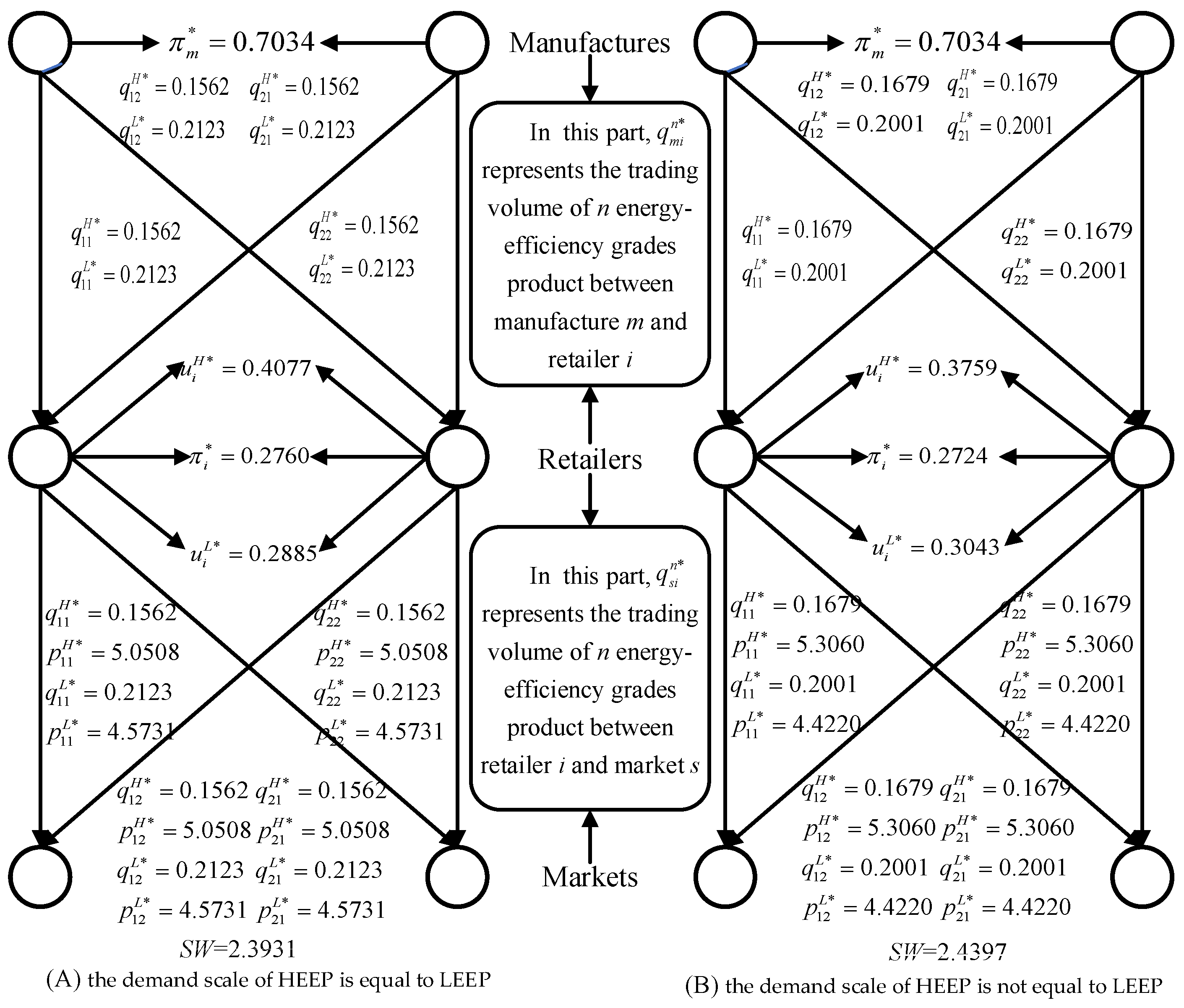
First, assuming that the energy-saving subsidies’ rate is zero, the effect of the demand scale difference on the equilibrium result of SCN is studied. When the demand scale of HEEP is equal to LEEP, that is $v_{si}^H=v_{si}^L=1$. Then, the equilibrium results are shown in Figure 4A. When the demand scale of HEEP is not equal to LEEP, that is $v_{si}^H=1.1;v_{si}^L=0.9$. Then, the equilibrium results are shown in Figure 4B.

Through Figure 4, we find that compared to when the demand scale of HEEP is equal to LEEP, when the demand scale of HEEP is larger, the transaction volume and transaction price of HEEP, the profits of manufacturers, the marketing efforts of retailers for LEEP, and social welfare are higher. The transaction volume, price of LEEP, the retailers’ profits, and HEEP’s marketing efforts are lower. Therefore, it is necessary to analyze the impact of energy-saving subsidy policy on SCNE in different situations.

Then, this paper supposes that the government subsidizes all HEEP sold by retailers in the market (There is no regional and object difference).

Table 3. The effect of $G_{si}^n$ on SCNE when the demand scales for HEEP and LEEP are equal.

Decision Variables	Energy-Saving Subside Rate ${\mathit{G}}_{\mathit{s}\mathit{i}}^{\mathit{n}}$
	0.00	0.05	0.10	0.15	0.20	0.25	0.30
$q_m^{1*}$	0.3124	0.3124	0.3124	0.3124	0.3124	0.3124	0.3124
$q_m^{2*}$	0.4246	0.4183	0.4128	0.4070	0.4022	0.3973	0.3927
$p_{si}^{1*}$	5.0508	4.9219	4.8018	4.6914	4.5887	4.4923	4.4038
$u_i^{1*}$	0.4077	0.4006	0.3938	0.3871	0.3804	0.3744	0.3681
$u_i^{2*}$	0.2885	0.3007	0.3123	0.3233	0.3336	0.3436	0.3528
${\pi }_m$	0.6813	0.6945	0.7074	0.7215	0.7356	0.7500	0.7654
${\pi }_i$	0.2760	0.2776	0.2801	0.2842	0.2893	0.2950	0.3023
SW	2.3931	2.3985	2.4010	2.4016	2.4002	2.3965	2.3917

and

Table 4. The effect of $G_{si}^n$ on SCNE when the demand scales for HEEP and LEEP are different.

Decision Variables	Energy-Saving Subside Rate ${\mathit{G}}_{\mathit{s}\mathit{i}}^{\mathit{n}}$
	0.00	0.05	0.10	0.15	0.20	0.25	0.30
$q_m^{1*}$	0.3358	0.3449	0.3538	0.3623	0.3707	0.3791	0.3872
$q_m^{2*}$	0.4002	0.3944	0.3885	0.3830	0.3778	0.3734	0.3688
$p_{si}^{1*}$	5.3060	5.1650	5.0360	4.9150	4.8040	4.7008	4.6048
$u_i^{1*}$	0.3759	0.3702	0.3645	0.3592	0.3537	0.3486	0.3435
$u_i^{2*}$	0.3043	0.3173	0.3294	0.3414	0.3523	0.3629	0.3727
${\pi }_m$	0.7034	0.7182	0.7342	0.7496	0.7660	0.7825	0.7999
${\pi }_i$	0.2724	0.2753	0.2797	0.2847	0.2911	0.2982	0.3064
SW	2.4397	2.4454	2.4489	2.4495	2.4486	2.4455	2.4408

show the SCN’s equilibrium results with equal and unequal demand scales, respectively.

Through Table 3, we find that the energy-saving subsidy rate is positively correlated with the transaction volume of HEEP, retailers’ marketing efforts for LEEP, and profits of manufacturers and retailers but negatively related to the transaction price of HEEP and the marketing efforts of retailers for HEEP. With the increase in the energy-saving subsidy rate, social welfare first increases and then decreases. When the energy-saving subsidy rate of HEEP is 0.15, the social welfare reaches the maximum.

Through Table 4, we find that with the increase of the HEEP’s subsidy rate, the transaction volume of HEEP and retailers’ marketing efforts for LEEP increase, while the transaction volume and price of LEEP and retailers’ marketing efforts for HEEP decrease. However, social welfare first increases and then decreases, reaching the maximum when $G_{si}^H=0.15$.

Compared with the demand scales for HEEP and LEEP when these are equal, the production, transaction price, retailer’s marketing efforts for LEEP, manufacturer’s profit, and social welfare are higher when the demand scales for HEEP and LEEP are different. The marketing efforts of retailers for HEEP and the retailer’s profit are relatively lower. Therefore, manufacturers prefer the government to adopt energy-saving subsidy incentives, while retailers do not always.

6. Discussion and Comparative Analysis

Due to the regional and object differences in energy-saving subsidies, there are many scenarios in practice. This section explores the influence of energy-saving subsidies on supply chain members’ decision-making and social welfare in different scenarios to provide more guidance for government and supply chain members in decision-making.

6.1. Scenarios When the Demand Scale for HEEP and LEEP Is Equal

Case 1. Government subsidizes HEEP sold by all retailers in market 1.

$G_{1i}^H$ is from 0 to 0.3. Other parameters and functions are the same as in Figure 3a in Section 5.2. With the increase of $G_{1i}^H$, the SCN’s equilibrium results are shown in

Table A1. The equilibrium result of government subsidies to all retailers in market 1 when demand scale for HEEP and LEEP is equal.

Decision Variables	Energy-Saving Subsidy Rate ${\mathit{G}}_{\mathit{s}\mathit{i}}^{\mathit{n}}$
	0.00	0.05	0.10	0.15	0.20	0.25	0.30
$q_m^{1*}$	0.3124	0.3168	0.3208	0.3246	0.3277	0.3307	0.3336
$q_m^{2*}$	0.4247	0.4213	0.4185	0.4164	0.4140	0.4119	0.4105
$q_{1i}^{1*}$	0.1562	0.1700	0.1837	0.1978	0.2122	0.2269	0.2416
$q_{2i}^{1*}$	0.1562	0.1468	0.1370	0.1267	0.1155	0.1038	0.0920
$p_{1i}^{1*}$	5.0508	4.9069	4.7741	4.6540	4.5413	4.4398	4.3477
$p_{2i}^{1*}$	5.0508	5.0625	5.0684	5.0701	5.0620	5.0510	5.0379
$u_i^{1*}$	0.4077	0.4040	0.4002	0.3958	0.3916	0.3867	0.3811
$u_i^{2*}$	0.2885	0.2944	0.2998	0.3045	0.3093	0.3132	0.3165
${\pi }_m$	0.6810	0.6873	0.6927	0.6984	0.7026	0.7075	0.7124
${\pi }_i$	0.2760	0.2768	0.2792	0.2835	0.2887	0.2966	0.3067
SW	2.3931	2.3950	2.3940	2.3907	2.3832	2.3732	2.3603

. Through Table A1, we find that energy-saving subsidy can increase HEEP’s transaction volume and reduce LEEP’s transaction volume. Retailers 1 and 2 will distribute more HEEP to market 1. With the increase of $G_{1i}^H$, the transaction price of HEEP in market 1 decreases. In contrast, the transaction price of HEEP in market 2 increases first and then decreases (When $G_{1i}^H<0.15$, the transaction price of HEEP in market 2 increases gradually and then decreases when it is higher than 0.15). However, the transaction price of HEEP in market 2 is always higher than that in market 1, indicating that government subsidies can benefit consumers. Besides, the higher $G_{1i}^H$ is, the higher the profits of manufacturers and retailers, and the lower the retailers’ marketing efforts to HEEP, while social welfare increased first and then decreased. When the $G_{1i}^H=0.05$, social welfare reaches the maximum.

Case 2. Government only subsidizes HEEP sold by retailer 1 in market 1.

$G_{11}^H$ belongs to interval [0, 0.3]. Other parameters and functions are same as Figure 3a in Section 5.2. With the increase of the energy-saving subsidy rate, the SCN’s equilibrium results are shown in

Table A2. The equilibrium result of government only subsidies to retailer 1 in market 1 when demand scale for HEEP and LEEP is equal.

Decision Variables	Energy-Saving Subsidy Rate ${\mathit{G}}_{\mathit{s}\mathit{i}}^{\mathit{n}}$
	0.00	0.05	0.10	0.15	0.20	0.25	0.30
$q_m^{1*}$	0.3124	0.3147	0.3171	0.3197	0.3222	0.3247	0.3273
$q_m^{2*}$	0.4247	0.4230	0.4214	0.4211	0.4206	0.4202	0.4193
$q_{11}^{1*}$	0.1562	0.1796	0.2018	0.2229	0.2430	0.2623	0.2808
$q_{21}^{1*}$	0.1562	0.1493	0.1428	0.1368	0.1311	0.1255	0.1201
$q_{12}^{1*}$	0.1562	0.1359	0.1171	0.0995	0.0833	0.0683	0.0545
$q_{22}^{1*}$	0.1562	0.1647	0.1726	0.1801	0.1870	0.1933	0.1992
$p_{11}^{1*}$	5.0508	4.9429	4.8415	4.7483	4.6592	4.5750	4.4975
$p_{21}^{1*}$	5.0508	5.0808	5.1103	5.1421	5.1715	5.2002	5.2303
$p_{12}^{1*}$	5.0508	4.9855	4.9241	4.8686	4.8150	4.7641	4.7178
$p_{22}^{1*}$	5.0508	5.0651	5.0802	5.0988	5.1162	5.1338	5.1540
$u_1^{1*}$	0.4077	0.3880	0.3693	0.3512	0.3342	0.3183	0.3032
$u_2^{1*}$	0.4077	0.4241	0.4405	0.4568	0.4735	0.4901	0.5057
${\pi }_m$	0.6810	0.6848	0.6898	0.6952	0.7013	0.7078	0.7164
${\pi }_1$	0.2760	0.2890	0.3039	0.3214	0.3398	0.3595	0.3813
${\pi }_2$	0.2760	0.2655	0.2570	0.2513	0.2465	0.2432	0.2416
SW	2.3931	2.3933	2.3906	2.3862	2.3791	2.3700	2.3599

. With the increase of $G_{11}^H$, the trading volume of HEEP increases, while that of LEEP decreases. The distribution quantity of HEEP of retailer 1 to market 1 is consistently highest. In market 1, retailer 2, which has no subsidy, has a higher transaction price for HEEP than retailer 1. Retailer 1’s marketing efforts for HEEP decrease, while retailer 2’s increase. However, with the increase of $G_{11}^H$, the profit of retailer 2 in market 1 declines and is eventually eliminated. Therefore, there is a time limit for government energy-saving subsidies, which is conducive to maintaining the diversification of the retailers. Besides, the profit of retailer 1 and manufacturers increases, and social welfare increases first and then decreases. When $G_{11}^H=0.05$, social welfare reaches the maximum.

6.2. Scenarios When the Demand Scales of HEEP and LEEP Is Different

Case 3. Government subsidizes HEEP sold by all retailers in market 1.

$G_{11}^H$ is from 0 to 0.3. Other parameters and functions are set the same as Figure 3b in Section 5.2. The equilibrium results of SCN are shown in

Table A3. The equilibrium result of government subsidies to all retailers in market 1 when demand scales of HEEP and LEEP is different.

Decision Variables	Energy-Saving Subsidy Rate ${\mathit{G}}_{\mathit{s}\mathit{i}}^{\mathit{n}}$
	0.00	0.05	0.10	0.15	0.20	0.25	0.30
$q_m^{1*}$	0.3359	0.3402	0.3442	0.3480	0.3513	0.3545	0.3573
$q_m^{2*}$	0.4006	0.3971	0.3947	0.3922	0.3901	0.3882	0.3865
$q_{1i}^{1*}$	0.1679	0.1819	0.1959	0.2102	0.2249	0.2399	0.2549
$q_{2i}^{1*}$	0.1679	0.1583	0.1483	0.1378	0.1265	0.1146	0.1024
$p_{1i}^{1*}$	5.3060	5.1500	5.0079	4.8799	4.7604	4.6520	4.5527
$p_{2i}^{1*}$	5.3060	5.3154	5.3210	5.3234	5.3166	5.3060	5.2918
$u_i^{1*}$	0.3759	0.3732	0.3701	0.3662	0.3625	0.3580	0.3533
${\pi }_m$	0.7030	0.7099	0.7159	0.7232	0.7288	0.7345	0.7400
${\pi }_i$	0.2724	0.2734	0.2766	0.2821	0.2884	0.2971	0.3079
SW	2.4397	2.4412	2.4403	2.4374	2.4302	2.4200	2.4062

. From Table A3, we find that with the increase of $G_{11}^H$, the transaction volume of HEEP and the distribution volume of retailers to market 1 increase; the transaction volume and price of LEEP decrease. For consumers in market 1, the higher the energy-saving subsidy, the better. However, for consumers of market 2, when the subsidy rate belongs to [0, 0.15], they do not want the government to subsidize market 1; when the subsidy rate belongs to [0.15, 0.3], consumers in market 2 hope that the higher the subsidy to market 1, the better. Although the transaction price is always higher than that of market 1, it is lower than market 1 without any energy-saving subsidy. No matter in which market, retailers’ marketing efforts for HEEP will decrease with the increase of $G_{11}^H$; the profits of manufacturers and retailers will increase; when $G_{11}^H=0.05$, social welfare reaches its maximum value.

Case 4. Government only subsidizes HEEP sold by retailer 1 in market 1.

The energy-saving subsidy rate $G_{11}^H$ is from 0 to 0.3, and other parameters and functions are set the same as Figure 3b in Section 5.2. The equilibrium results of SCN are shown in

Table A4. The equilibrium result of government only subsidies to retailer 1 in market 1 when demand scales of HEEP and LEEP is different.

Decision Variables	Energy-Saving Subsidy Rate ${\mathit{G}}_{\mathit{s}\mathit{i}}^{\mathit{n}}$
	0.00	0.05	0.10	0.15	0.20	0.25	0.30
$q_m^{1*}$	0.3359	0.3382	0.3405	0.3432	0.3457	0.3485	0.3512
$q_m^{2*}$	0.4006	0.3987	0.3975	0.3969	0.3960	0.3955	0.3953
$q_{11}^{1*}$	0.1679	0.1923	0.2155	0.2376	0.2587	0.2790	0.2984
$q_{21}^{1*}$	0.1679	0.1605	0.1534	0.1470	0.1407	0.1348	0.1290
$q_{12}^{1*}$	0.1679	0.1466	0.1268	0.1085	0.0914	0.0756	0.0611
$q_{22}^{1*}$	0.1679	0.1769	0.1853	0.1933	0.2007	0.2076	0.2140
$p_{11}^{1*}$	5.3060	5.1908	5.0825	4.9845	4.8902	4.8038	4.7214
$p_{21}^{1*}$	5.3060	5.3359	5.3651	5.3984	5.4288	5.4613	5.4921
$p_{12}^{1*}$	5.3060	5.2355	5.1691	5.1106	5.0536	5.0022	4.9528
$p_{22}^{1*}$	5.3060	5.3192	5.3330	5.3520	5.3694	5.3900	5.4099
$u_1^{1*}$	0.3760	0.3572	0.3395	0.3221	0.3060	0.2906	0.2763
$u_2^{1*}$	0.3760	0.3924	0.4089	0.4252	0.4419	0.4580	0.4740
${\pi }_m$	0.7030	0.7074	0.7121	0.7188	0.7259	0.7344	0.7429
${\pi }_1$	0.2724	0.2870	0.3036	0.3233	0.3439	0.3668	0.3907
${\pi }_2$	0.2724	0.2606	0.2512	0.2449	0.2397	0.2365	0.2343
SW	2.4397	2.4396	2.4363	2.4315	2.4236	2.4144	2.4030

. With the increase of $G_{11}^H$, the trading volume of HEEP between market 1 and retailer 1 increases. Due to subsidy and price competition, the transaction prices of HEEP in market 1 decrease. In addition, the distribution quantity of HEEP from retailer 1 to market 2 is reduced, and the demand exceeds supply, increasing transaction price. Retailer 1’s marketing efforts on HEEP decrease, contrary to retailer 2. The profit of manufacturers and retailer 1 increases, while the profit of retailer 2 and social welfare decrease.

6.3. Comparative Analysis

Comparing case 1 and case 3, we found that when the demand scales of HEEP and LEEP are different, the equilibrium price of HEEP, manufacturers’ profit, and social welfare are higher. Moreover, the profit and marketing efforts for HEEP of retailers are lower. Consumers in market 2 prefer that the government not subsidize market 1, or the subsidy rate is 0.3. It can be seen that the energy-saving subsidy policy of market 1 cannot only intervene in the decision-making of market 1, but also affect the decision-making of other markets.

Compared with cases 2 and 4, we find that, regardless of the demand scale, when the government only subsidizes the HEEP sold by some retailers, the gap between subsidized and non-subsidized retailers is widened. As a result, the profits of retailers eligible for government subsidies are higher, and those not eligible for government subsidies are lower, which will encourage retailers to enhance their strength to meet the qualification of sales enterprises.

6.4. Extensions

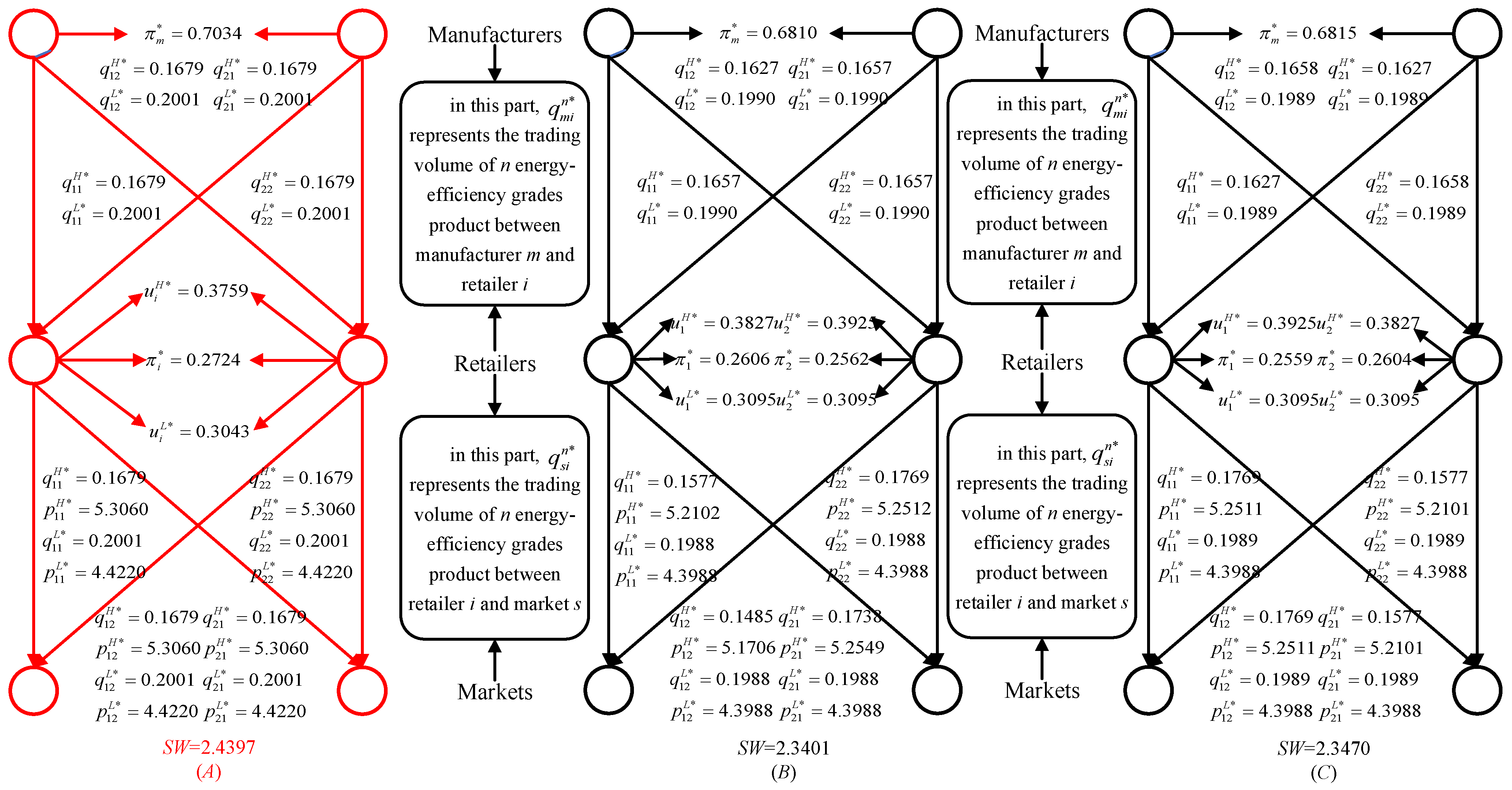
Retailers have different services for different markets, such as remote areas are not free distribution; delivery outside the jurisdiction is not free. Therefore, we assume that the demand scales for retailers are different, explore the impact of government subsidies on the SCNE results, and provide an essential reference for retailers. First, we assume three scenarios: scenario A: there is no difference in the demand scale of the same retailer in the same market; scenario B: different retailers in the same market have different demand scales. (The demand scale of market 1 to retailer 1 and retailer 2 is different, and the demand scale of market 1 to retailer 2 is small); scenario C: different markets have different demand scales for the same retailer (The demand scale of market 1 and market 2 for retailer 1 is different, and market 2 has a smaller demand scale for retailer 1).

When the government does not implement the subsidy policy, the equilibrium results among the members of the SCN are shown in Figure 5. Figure 5B is obtained when $v_{11}^H=1.1;v_{12}^H=1;v_{si}^L=0.9$ and other parameters are set the same as Figure 4B. Figure 5C is obtained when $v_{11}^H=1.1;v_{21}^H=1;v_{si}^L=0.9$ and other parameters are set the same as Figure 4B; all parameters in Figure 5A are set the same as Figure 4B.

Figure 5 shows that, compared with scenario A, the profit of manufacturers and retailers, product production, and the transaction price between retailers and markets are lower than in situations B and C. In contrast, the retailer’s marketing efforts for HEEP and LEEP are higher, which is consistent with the previous conclusion; the retailers with higher demand scales have lower marketing efforts. In addition, we find that the demand scale positively correlates with the equilibrium price compared to situations B and C. Therefore, government subsidies are essential for the SCNE with multi-energy efficiency products for different scenarios. Therefore, it is necessary to analyze the effect of government subsidies on the SCNE with multi-energy efficiency products in different scenarios.

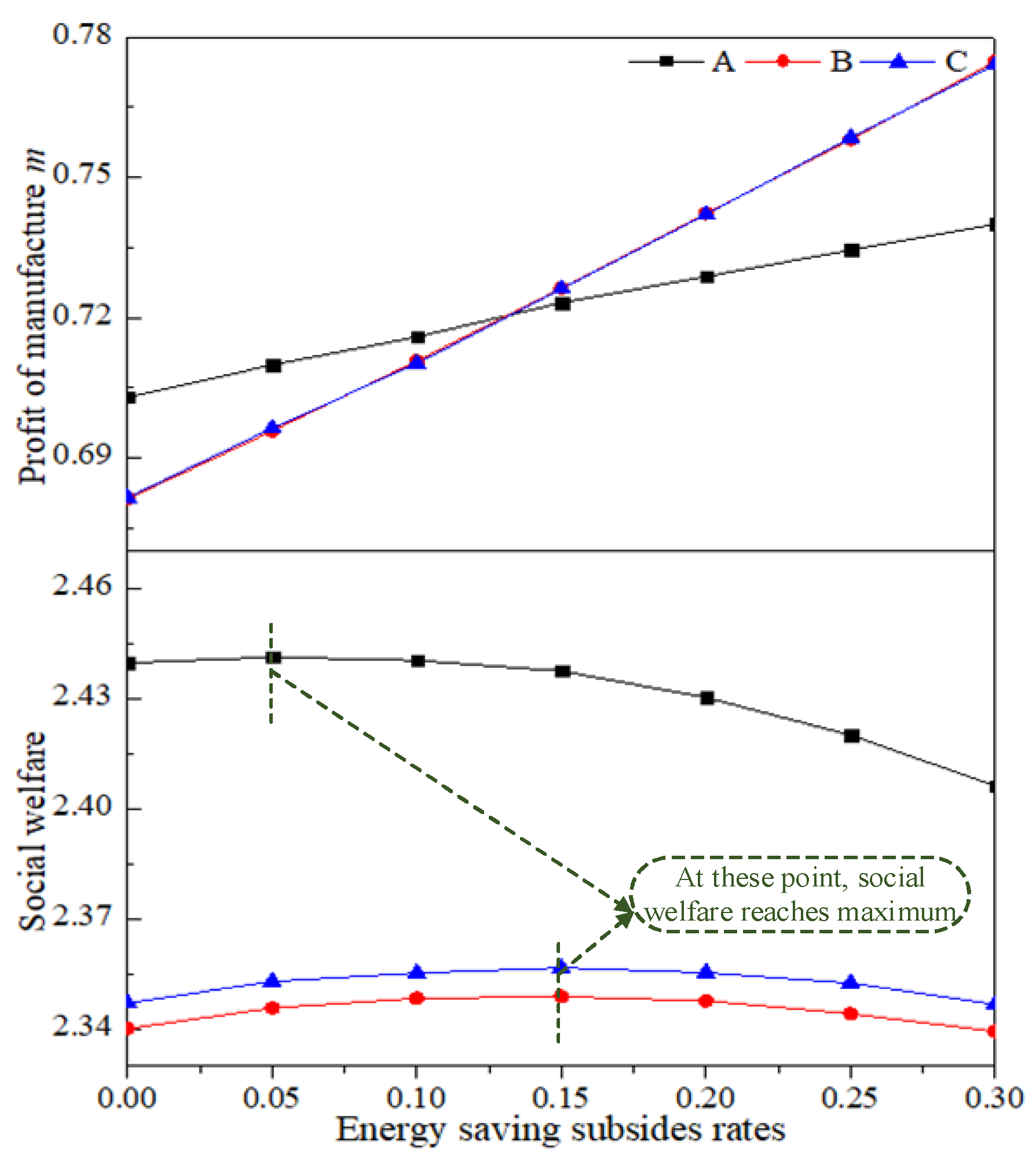
Then we set $G_{si}^H\in [0,0.3]$ and make a comparative analysis with scenario B and C and case 3 (scenario A). The following conclusions are obtained through calculation: with the increase of subsidy, the production of HEEP increases in scenarios B and C, but are still smaller than that in case 3; the production of LEEP is undifferentiated. The profits of manufacturers and retailers, HEEP’s marketing efforts, and social welfare are shown in Figure 6 and Figure 7.

Through Figure 6, we find that with the increase of $G_{si}^H$, manufacturers’ profits increase, and the profits of manufacturers in scenarios B and C are close. When $G_{si}^H<0.15$, the manufacturer’s profit in scenario A is higher; when the subsidy is greater than 0.15, its profit is higher in scenarios B and C. The optimal subsidy rate of social welfare is different in different scenarios. In scenario A, the social welfare is the largest when $G_{si}^H=0.05$, and the optimal social welfare rate is 0.15 in scenarios B and C, which is close to the energy-saving subsidy rate in reality. It shows that the market structure in real life is more similar to scenarios B and C (There are differences in demand scale and government subsidies.).

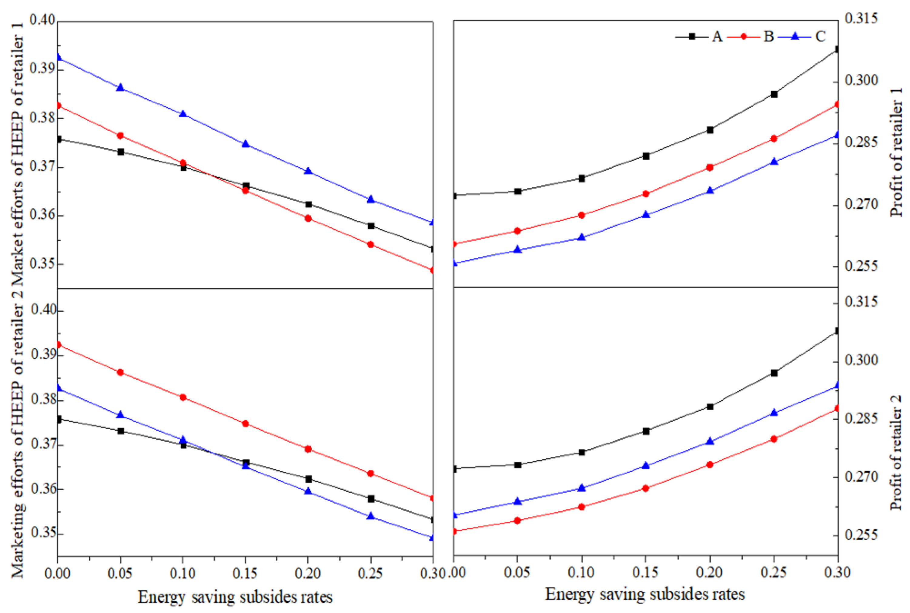
Through Figure 7, we find that with the increase of $G_{si}^H$, retailers’ profits increase, and HEEP’s marketing efforts decline. When $G_{si}^H<0.15$, the retailer’s marketing efforts for HEEP are the lowest in situation C. The demand scale is negatively correlated with the marketing efforts of subsidized retailers for HEEP and positively correlated with the marketing efforts of non-subsidized retailers for HEEP in the same market. Compared with situation C, retailers’ profit gap in situation B is more prominent, which is more conducive to eliminating retailers with lower demand scales.

6.5. Management Insights

Saving resources is the primary national policy of our country. China implements the energy development strategy of conservation and development simultaneously and puts conservation in first place. As an essential branch of energy consumption, the government has also issued relevant policies to encourage consumers to use energy-saving appliances. Based on this, the paper studies the impact of energy-saving subsidy policy on the decision-making of each SCN member in different scenarios and puts forward the following suggestions for enterprise managers:

In terms of methods, based on variational inequality theory and game theory, this paper constructs a multi-energy-efficiency-grade equilibrium model to maximize the supply chain members’ profit and uses the Euler algorithm to solve the model, which enriches the theoretical research in the operational research field and provides an essential theoretical basis for enterprise decision-making. The increase in demand scale and subsidy rate of HEEP will increase manufacturers’ profits. On the one hand, manufacturers can reduce the production costs of products and increase their profits. On the other hand, manufacturers can share the cost of marketing efforts with retailers to encourage retailers to expand HEEP’s demand scale. For retailers, the increase of energy-saving subsidies will increase the retailer’s profit when there is no difference between subsidy region and object; however, when there is a difference between subsidy and object, the retailer’s profit fails to meet the subsidy qualification will decrease. Therefore, retailers should strive to improve their own strength to meet the government’s requirements for the operation of subsidized products. Besides, retailers should improve their market demand scale. For the government, the subsidy policies adopted in different scenarios should be different, and the threshold for retailers to sell HEEP should be formulated scientifically.

7. Conclusions

Regarding our first question, we find that energy-saving subsidies can increase HEEP’s trading volume, reduce the transaction volume of LEEP, and increase the price competition between products. In the same market, energy-saving subsidies and demand scales are all negatively correlated with the marketing efforts of subsidized retailers for HEEP and positively correlated with the marketing efforts of non-subsidized retailers for HEEP. In contrast, the marketing efforts for LEEP are the opposite. The demand scale and energy-saving subsidy of HEEP positively correlate with manufacturers’ profits, which is not always the case for retailers. With respect to our second research question, we discover that different demand scales lead to different equilibrium prices of the same product in the same market. The increase in demand scale and energy-saving subsidies of HEEP can increase manufacturers’ profits, which is not always the case for retailers. When there is no regional and object difference in subsidies, the government subsidy rate is 0.15, and social welfare is the largest; otherwise, when the government subsidy rate is 0.05, the social welfare is the largest. Through the expansion, we find that the retailers in the same market always tend to be consistent in development, which is counterintuitive. We also discover that the differentiation of market demand scale will eliminate the retailers without a competitive advantage.

This paper only considers government subsidies for energy-efficient products. In future research, we will consider subsidizing multiple products of retailers at the same time to explore the influence of energy-saving subsidy policies on the equilibrium decision-making of SCN members.

References

1. He, L.; Lo, K.; Wang, M.; Zhang, P.; Xue, L. Industrial energy consumption in northeast china under the revitalization strategy: A decomposition and policy analysis. Energies 2016, 9, 549. [Google Scholar] [CrossRef] [Green Version]
2. Zhang, F.; Wang, H.; Wu, X. The impact of government subsidies on single-channel recycling based on recycling propaganda. Energies 2021, 14, 8189. [Google Scholar] [CrossRef]
3. Huang, W.; Zhou, W.; Chen, J.; Chen, X. The government’s optimal subsidy scheme under Manufacturers’ competition of price and product energy efficiency. Omega 2019, 84, 70–101. [Google Scholar] [CrossRef]
4. Li, X.; Li, Y. On green market segmentation under subsidy regulation. Supply Chain Manag. 2017, 22, 284–294. [Google Scholar] [CrossRef]
5. Helveston, J.P.; Liu, Y.M.; Feit, M.D.; Fuchs, E.; Klampfl, E.; Michalek, J.J. Will subsidies drive electric vehicle adoption? Measuring consumer preferences in the U.S. and China. Transp. Res. A-POL 2015, 73, 96–112. [Google Scholar] [CrossRef] [Green Version]
6. Shao, L.L.; Yang, J.; Zhang, M. Subsidy scheme or price discount scheme? Mass adoption of electric vehicles under different market structures. Eur. J. Oper. Res. 2017, 3, 1181–1195. [Google Scholar] [CrossRef]
7. Barre, R. Galbraith (JK)-American Capitalism: The Concept of Countervailing Power; Houghton Mifflin: New York, NY, USA, 1954; Volume 5, pp. 324–325. [Google Scholar]
8. Yi, Y.Y.; Li, J.X. The effect of governmental policies of carbon taxes and energy-saving subsidies on enterprise decisions in a two-echelon supply chain. J. Clean. Prod. 2018, 181, 675–691. [Google Scholar]
9. Bao, B.; Ma, J.; Goh, M. Short-and long-term repeated game behaviours of two parallel supply chains based on government subsidy in the vehicle market. Int. J. Prod. Res. 2020, 58, 7507–7530. [Google Scholar] [CrossRef]
10. Cao, K.; He, P.; Liu, Z. Production and pricing decisions in a dual-channel supply chain under remanufacturing subsidy policy and carbon tax policy. J. Oper. Res. Soc. 2020, 71, 1199–1215. [Google Scholar] [CrossRef]
11. Fu, J.; Chen, X.; Hu, Q. Subsidizing strategies in a sustainable supply chain. J. Oper. Res. Soc. 2017, 1–14. [Google Scholar] [CrossRef]
12. Aydin, E.; Brounen, D. The impact of policy on residential energy consumption. Energy 2019, 169, 115–129. [Google Scholar] [CrossRef]
13. Zhang, H.M.; Li, L.S.; Zhou, P.; Hou, J.M.; Qiu, Y.M. Subsidy modes, waste cooking oil and biofuel: Policy effectiveness and sustainable supply chains in China. Energy Policy 2014, 65, 270–274. [Google Scholar] [CrossRef]
14. Krass, D.; Nedorezov, T.; Ovchinnikov, A. Environmental Taxes and the Choice of Green Technology. Prod. Oper. Manag. 2013, 22, 1035–1055. [Google Scholar] [CrossRef]
15. Bi, G.; Jin, M.; Ling, L.; Yang, F. Environmental subsidy and the choice of green technology in the presence of green consumers. Ann. Oper. Res. 2017, 255, 547–568. [Google Scholar] [CrossRef]
16. Madam, S.R.; Rasti-Barzoki, M. Sustainable Supply Chain Management with Pricing, Greening and Governmental Tariffs Determining Strategies: A Game-theoretic Approach. Comput. Ind. Eng. 2017, 105, 287–298. [Google Scholar] [CrossRef]
17. Taylor, T.A. Supply Chain Coordination under Channel Rebates with Sales Effort Effects. Manag. Sci. 2002, 48, 992–1007. [Google Scholar] [CrossRef] [Green Version]
18. Song, J.; Li, F.; Wu, D.D.; Liang, L.; Dolgui, A. Supply chain coordination through integration of innovation effort and advertising support. Appl. Math. Model. 2017, 49, 108–123. [Google Scholar] [CrossRef]
19. Ma, J.; Zhang, D.; Dong, J.; Tu, Y. A supply chain network economic model with time-based competition. Eur. J. Oper. Res. 2020, 280, 889–908. [Google Scholar] [CrossRef]
20. Li, Q.; Sun, H.; Zhang, H.; Li, W.; Ouyang, M. Design Investment and Advertising Decisions in Direct-Sales Closed-Loop Supply Chains. J. Clean. Prod. 2019, 250, 119552. [Google Scholar] [CrossRef]
21. Sarkar, B.; Omair, M.; Kim, N. A cooperative advertising collaboration policy in supply chain management under uncertain conditions. Appl. Soft Comput. 2019, 88, 105948. [Google Scholar] [CrossRef]
22. Nagurney, A.; June, D. A multiclass, multicriteria traffic network equilibrium model with elastic demand. Transp. Res. B-Methodol. 2002, 36, 445–469. [Google Scholar] [CrossRef]
23. Nagurney, A.; Cruz, J.; Dong, J.; Zhang, D. Supply chain networks, electronic commerce, and supply side and demand side risk. Eur. J. Oper. Res. 2005, 164, 120–142. [Google Scholar] [CrossRef]
24. Nagurney, A.; Trisha, W.; Qiang, Q. Multi-product supply chain horizontal network integration: Models, theory, and computational results. Int. Trans. Oper. Res. 2010, 17, 333–349. [Google Scholar] [CrossRef] [Green Version]
25. Valderrama, C.V.; Santibanez-González, E.; Pimentel, B.; Candia-Véjar, A.; Canales-Bustos, L. Designing an environmental supply chain network in the mining industry to reduce carbon emissions. J. Clean. Prod. 2020, 254, 119688. [Google Scholar] [CrossRef]
26. Saberi, S.; Cruz, J.M.; Sarkis, J.; Nagurney, A. A competitive multiperiod supply chain network model with freight carriers and green technology investment option. Eur. J. Oper. Res. 2018, 266, 934–949. [Google Scholar] [CrossRef]
27. Li, D.; Nagurney, A. A general multitiered supply chain network model of quality competition with suppliers. Int. J. Prod. Econ. 2015, 170, 336–356. [Google Scholar] [CrossRef]
28. Yu, M.; Nagurney, A. Competitive food supply chain networks with application to fresh produce. Eur. J. Oper. Res. 2013, 224, 273–282. [Google Scholar] [CrossRef]
29. Qiang, Q.; Ke, K.; Anderson, T.; Dong, J. The closed-loop supply chain network with competition, distribution channel investment, and uncertainties. Omega 2013, 41, 186–194. [Google Scholar] [CrossRef]
30. Rahemi, H.; Torabi, S.A.; Avami, A.; Jolai, F. Bioethanol supply chain network design considering land characteristics. Renew. Sustain. Energy Rev. 2020, 119, 109517. [Google Scholar] [CrossRef]
31. Alizadeh, M.; Makui, A.; Paydar, M.M. Forward and reverse supply chain network design for consumer medical supplies considering biological risk. Comput. Ind. Eng. 2020, 140, 106229. [Google Scholar] [CrossRef]
32. Fragoso, R.; Figueira, J.R. Sustainable supply chain network design: An application to the wine industry in Southern Portugal. J. Oper. Res. Soc. 2021, 72, 1236–1251. [Google Scholar] [CrossRef]
33. Park, K.; Kim, J.; Ko, Y.D.; Song, B.D. Redesign of reverse logistics network with managerial decisions on the minimum quality level and remanufacturing policy. J. Oper. Res. Soc. 2021, 72, 1564–1577. [Google Scholar] [CrossRef]
34. Nagurney, A. Network Economics: A Variational Inequality Approach; Springer Science & Business Media: Berlin/Heidelberg, Germany, 1998. [Google Scholar]
35. Hammond, D.; Beullens, P. Closed-loop supply chain network equilibrium under legislation. Eur. J. Oper. Res. 2007, 183, 895–908. [Google Scholar] [CrossRef]
36. Liu, Z.; Jia, W. Supply chain network equilibrium with strategic financial hedging using futures. Eur. J. Oper. Res. 2019, 272, 962–978. [Google Scholar] [CrossRef]
37. Nagurney, A.; Zhang, D. Projected Dynamical Systems and Variational Inequalities with Applications; Springer Science & Business Media: Berlin/Heidelberg, Germany, 1995. [Google Scholar]
38. Chen, Z.; Tian, C.; Zhang, D.; Chen, D. Dynamic model of a supply chain network with sticky price. Oper. Res. 2020, 20, 649–670. [Google Scholar] [CrossRef]
Figure 1. SCN structure.
Energies 15 07376 g001
Figure 2. Roadmap.
Energies 15 07376 g002
Figure 3. Frame diagram of the numerical example.
Energies 15 07376 g003
Figure 4. The results of SCNE in different market scales.
Energies 15 07376 g004
Figure 5. When the subsidy rate is 0, the SCNE results in different scenarios. (A) there is no difference in the demand scale of the same retailer in the same market. (B) different retailers in the same market have different demand scales. (C) different markets have different demand scales for the same retailer.
Energies 15 07376 g005
Figure 6. The SCNE results of manufacturer m’s profit and social welfare in different scenarios.
Energies 15 07376 g006
Figure 7. The SCNE results of retailer i’s profit and marketing efforts for HEEP in different scenarios.
Energies 15 07376 g007