Article

The Applicability of Biogeography-Based Optimization and Earthworm Optimization Algorithm Hybridized with ANFIS as Reliable Solutions in Estimation of Cooling Load in Buildings

1
Institute of Research and Development, Duy Tan University, Da Nang 550000, Vietnam
2
School of Engineering & Technology, Duy Tan University, Da Nang 550000, Vietnam
*
Author to whom correspondence should be addressed.
Energies 2022, 15(19), 7323; https://doi.org/10.3390/en15197323
Submission received: 28 August 2022 / Revised: 29 September 2022 / Accepted: 1 October 2022 / Published: 5 October 2022

Abstract

:
The foundation of energy-efficient architectural design is modeling heating and cooling loads (HLs and CLs), which defines the heating and cooling apparatus constraints necessary to maintain a suitable interior air environment. It is possible that analytical models for energy-efficient buildings might offer an accurate evaluation of the influence that various building designs would have. The implementation of these instruments, however, might be a process that requires a significant amount of manual labor, a significant amount of time, and is reliant on user experiences. In light of this, the authors of this paper present two unique methods for estimating the CL of residential structures in the form of complex mathematical concepts. These methodologies include an evolutionary web algorithm (EWA), biogeography-based optimization (BBO), and a hybridization of an adaptive neuro-fuzzy interface system (ANFIS), namely BBO-ANFIS and EWA-ANFIS. The findings initiated from each of the suggested models are evaluated with the help of various performance metrics. Moreover, it is possible to determine which model is the most effective by comparing their coefficient of determination ( R 2   ) and its root mean square error (RMSE) to each other. In mapping non-linear connections between input and output variables, the observed findings showed that the models used have a great capability. In addition, the results showed that BBO-ANFIS was the superior forecasting model out of the two provided models, with the lowest value of RMSE and the greatest value of R 2   (RMSE = 0.10731 and 0.11282 and R 2   = 0.97776 and 0.97552 for training and testing phases, respectively). The EWA-ANFIS also demonstrated RMSE and R 2   values of 0.18682 and 0.17681 and 0.93096 and 0.93874 for the training and testing phases, respectively. Finally, this study has proven that ANN is a powerful tool and will be useful for predicting the CL in residential buildings.

1. Introduction

It is envisioned that buildings will be constructed to decrease the amount of both materials and energy while simultaneously optimizing the security and well-being of the people living in them. In order to accomplish this objective, it is recommended that both new energy-efficient buildings be built and improvements be made to already existing buildings. Because of the persistently negative effects of energy waste on the surrounding environment, a considerable amount of attention and effort has been directed toward studying the energy performance of buildings (EPB) [1,2,3]. In addition, statistics showed that recent decades witnessed a significant rise in global energy usage, heating, ventilation, and air conditioning (HVAC), accounting for the majority of this growth as indoor temperature controllers [4,5]. Consequently, offering better energy-efficient building designs with updated energy-saving features is one strategy to lessen the ever-increasing demand for increased power generation [6]. This may be performed by reducing the energy wasted in buildings [7,8,9].
The ability to accurately forecast how much energy a building will use is critical for improving that facility’s energy efficiency and, ultimately, lowering its environmental effect. Because of the introduction of an unprecedented thermal regulation in the inhabited and tertiary building sectors in Morocco in the last several years, there has been a considerable rise in the urgency with which the country’s buildings must achieve much higher levels of energy effectiveness. It is vital to calculate the HLs and CLs while designing the building so that the air conditioning system requirements may be determined in order to retain suitable interior thermal conditions.
The foundation of energy-efficient architectural design is modeling HLs and CLs, which define the heating and cooling apparatus constraints necessary to maintain a suitable interior air environment. Because they make it feasible to conduct experiments with variables that, in the real world, would normally be either impossible or extraordinarily challenging to manage, simulation tools are extremely popular across many different fields [10,11]. It is feasible to create energy-efficient buildings by using technologies such as BPS, which employs a simulation platform that relies on physical principles to predict the energy requirements of the structure [12]. Before development ever begins, BPS calculates the building’s potential energy savings by considering the influence of the building’s materials, systems, and shape [13,14].
According to Zhao et al., many different ways may be used to anticipate the energy required for buildings [15]. Some of these strategies include physical, statistical, regression, and artificial intelligence [16,17,18]. When determining the equilibrium state of buildings, physical techniques, which are established upon physical engineering approaches and make utilization of thermodynamic and heat transport features, are often used [19,20]. EnergyPlus [21], ESP-r [22], IBPT [23], SIMBAD [24], TRNSYS [25], and CARNOT [26] are only a few of the physical building simulation implements created in recent years. The application of these instruments calls for the laborious effort of trained professionals, resulting in a challenging implementation that comes at a serious expense [27]. Because of these factors, a number of scholars have suggested more straightforward methods to address this issue [28,29].
Ongoing research has looked at the possibility of modeling the energy performance of buildings (EBP) by making predictions about the HL and CL using soft computing techniques. Artificial neural networks (ANNs) were used by Kalogirou et al. [30] in order to estimate the everyday energy needs of vacation homes as well as the day-to-day HLs of model house constructions that included a variety of wall and roof configurations [31]. Yokoyama et al. [18] utilized ANN in conjunction with an optimization strategy to make an accurate prediction of the CL need. In order to predict the need for heating in dwellings, Catalina et al. [32] used a polynomial regression with five distinct variables as inputs. A support vector machine (SVM) was used by Dong et al. [33] to evaluate CL daily in dwellings. An artificial neural network (ANN) technique related to heat convection was established by Zhang and Haghighat [34] for the thermal modeling of square-shaped cross-sectional surface earth-to-earth heat exchanges. Yu et al. [1] introduced a decision tree technique to model the energy need of buildings. Deb et al. [35] made their predictions on the daily CL for official erections using ANN. Bioclimatic buildings have been studied by Mena et al. [36], who used an ANN-based predictive model to estimate their energy use. A principle component analysis (PCA) linked to an artificial neural network (ANN) was created by Platon et al. [37] to forecast the daily power usage of a house [38]. PCA was also used by Li 116 and colleagues [39] to optimize the number of input factors to forecast the amount of power a building will use. Random forest (RF) was the methodology that Tsanas and Xifara [2] utilized to estimate dwellings’ power requirements. ANN was used by Hong et al. [40] and Khayatian and Sarto [41] in order to analyze the energy performance of a school located in the United Kingdom and structures located in Italy. Seyedzadeh et al. [9] used machine learning (ML) algorithms that were fine-tuned before the modeling process began to accurately predict the building’s energy demands [42].
As is evident from the earlier cases, many different models utilizing artificial intelligence (AI) were employed in order to make predictions about the EPB. Though hybrid and fuzzy logic-based models are still developing, nothing is known about how they may be used to simulate housing structures’ HLs and CLs. Moreover, finding research that is both thorough and comparable to modern soft computing approaches is still not possible. In addition, there has not yet been a comprehensive assessment of the statistical analysis performed on the data produced from the models. This research was prompted to create two sophisticated analytical systems comprising an evolutionary web algorithm (EWA), biogeography-based optimization (BBO), and a hybrid adaptive neuro-fuzzy interface (ANFIS), i.e., BBO-ANFIS and EWA-ANFIS, which are well-recognized for their great comprehensiveness and low computing expense as replacements for standard computer simulations to predict housing building CLs of 768 examples of dwellings.
The following is the order in which this document is structured: Following the introduction comes part 2, which has an overview of the information and its distribution. Part 3 follows with a discussion of the conceptual framework of the models that were used, hybridization processes, and the creation of the methodology used in this research. The findings of this research are then thoroughly analyzed using a wide variety of statistical factors and methods of analysis to assess the modeling performance of the models presented in part 4. This study is brought to a close with some reflections on the findings in Part 5.

2. Established Database

This part provides a full overview of the extensive dataset utilized for this research project. The information used for the present investigation was obtained from Tsanas and Xifara [2], consisting of 768 data points. A total of eight factors are taken into account while building a model, which consist of relative compactness (RC), surface area (SA), wall area (WA), roof area (RA), overall height (OH), orientation (OR), glazing area (GA), glazing area distribution (GAD), and the output variable of CL. The statistical values of both the input and output variables are given in Table 1.
On the basis of floor space, three glazing percentages were contemplated, ranging from 10% to 25% to 40%. In addition, simulations were performed using the following distinct distribution possibilities for every single glazing area: It is homogeneous on all sides, with 25% glazing on every single side; it is 55% on the north and 15% on the each sides; it is 55% for the east; it is 55% for the south; it is 55% for the west; and it is 15% for all other sides for the south. In addition, we were able to collect specimens that did not have any glazing regions. After that, each form was turned to face one of the four fundamental directions (see Figure 1).

3. Methodology

In this investigation, the energy efficiency of dwellings is modeled by forecasting the amount of CL required, and two sophisticated computational systems, notably BBO-ANFIS and EWA-ANFIS, are utilized to do so. The next subcategories detail both the theoretical foundations of the aforementioned models and the methodological advancements that were made in their creation.

3.1. Adaptive Neuro-Fuzzy Interface System (ANFIS)

Soft computing approaches, such as neural networks and fuzzy set theory, are examples of instruments that may be used to establish intelligent systems. This hypothesis offers a fresh approach to resolving the problem that the probability hypothesis was unable to shed light on [43]. Additionally, the knowledge provided by humans is necessary for this system. Fuzzy rules are regularly included in the fuzzy deduction framework, the most well-known kind of fuzzy structure and a fuzzy examination. For the most part, rules may be seen as the following: They include phonetic factors and fuzzy recommendations.
I f P r e m i s e   P r o p o s i t i o n   p T h e n   C o n s e q u e n t   P r o p o s i t i o n   q
Sometimes when rules are imposed through regulators in the fuzzy interface system (abbreviated as FIS), but in the adaptable neuro-fuzzy interface system (abbreviated as ANFIS), these rules spontaneously establish suitable criteria for the data that are input and the data that are yielded, and they stimulate the learning powers of neural systems [44,45]. When a rule cannot be adhered to for whatever reason, it ought to be removed. In every other case, it will be factored into the equation. In this manner, the neural network achieves its optimal state. It is important to note that the first phase is referred to as training, and at this stage, the model shows the ideal system with the smallest amount of error that is even remotely possible, as shown in the network diagram [46].
The goal is to improve performance while simultaneously reducing mistake rates and characterizing relevant error functions and indices [47]. Fuzzy if–then rules with two inputs and one output may be expressed as.
First   rule ,   if   x = A 1   and   y = B 1   then   f 1 = p 1 x + q 1 y + r 1
Sec ond   rule ,   if   x = A 2   and   y = B 2   then   f 2 = p 2 x + q 2 y + r 2
In which x and y denote the inputs; A 1 , A 2 , B 1 , and B 2   designate the phonological labels; p and q present the resultant factors; and f shows the output in fuzzy. Figure 2 depicts the first-order Takagi–Sugeno Fuzzy Model’s modified ANFIS architecture.
In which x and y represent the input or passive layer and the membership function, rule layer, norm layer, output layer, and final output layer represent the first, second, third, fourth, and fifth layers, respectively.

3.2. Biogeography-Based Optimization (BBO)

Biogeography is an interdisciplinary branch of life and earth knowledge that examines wild communities’ dispersal, relocation, and extinction within their respective areas [48]. Within the context of this tactic, every creature has its own specific ecological value, which is denoted by the environmental appropriateness indicator. The environmental appropriateness indicator shows the degree of its pleasure or quality. The fundamental aspects of biogeography-based optimization, also known as BBO, are the migration of characteristics from high to low and the acquisition of fresh characteristics moving in the opposite direction, from low to high. It is possible to arrive at the optimal answer by repeating the method described previously [49]. The following is a description of the two primary operators of this algorithm, which are migration and mutation:
Migration: Information may be sent from one solution to the next through the operator; however, this is contingent upon two parameters representing the movement and migration rates and is specified hereunder:
λ k = λ m a x 1 k k m a x
μ k = μ m a x k k m a x
In which λ k   and μ k   denote the rates of immigration and emigration and k designates the solution’s rank. According to the model presented above, the rates of immigration and emigration are equal under the conditions of having the greatest number of distinct species ( S m a x ).
Mutation: Because tragedies or illnesses induce alterations in the coefficients of the solution, the concept of transformation may be seen as an unforeseen variation in species. The following equation may be used to express the mutation value of species:
m k = m m a x 1 P k P m a x
In which the m k   and m m a x   denote the mutation rates, P k   and P m a x   designate every one of species’ likelihood, and k presents the solution’s rank. The   P k   is expressed as follows:
p k = λ k + μ k P k + μ k + 1 P k + 1                         k = 0 λ k + μ k P k + λ k 1 P k 1 + μ k + 1 P k + 1                         1 k k m a x 1 λ k + μ k P k + λ k 1 P k 1                                 k = k m a x

3.3. Earthworm Optimization Algorithm (EWA)

In order to find solutions to optimize issues, EWA is a “nature-inspired evolutionary algorithm” that is based on the reproductive process of earthworms [50]. To use EWA, you must follow the following rules: (A) There are only two distinct modes of reproduction available to earthworms in the population, and every single earthworm is capable of producing offspring through any of these methods. (B) An identical set of DNA strands may be found in both parents and children of a similar earthworm. (C) A number of the earthworms from the earlier generations that were in the finest physical condition are passed on unchanged to the following generation. An overview of “EWA” is provided below.
(1).
Reproduction 1
Hermaphrodites are found in the earthworm family. That indicates that every single one of them possesses both male and female genitalia inside their bodies. This means that a single parent earthworm is capable of producing an entirely independent offspring earthworm. The following is a mathematical description of Reproduction 1.
u i 1 , k = u m a x , k + u m i n , k α u i , k
The aforementioned equation details the process that must be followed in order to produce the kth element of infant earthworm i1 using earthworm i as the parent. The symbols u i 1 , k and u i , k   denote the kth element of earthworm i1 and i, respectively. The operational limitations of the kth element of each earthworm are denoted by u m a x , k   and u m i n , k , respectively. The “similarity factor”, whose value may range anywhere from 0 to 1, decides the amount of genetic material passed down from the parent earthworm to the offspring.
(2).
Reproduction 2
The “single-point crossover”, “multipoint crossover”, and “uniform crossover” operators used in Reproduction 2 are upgraded versions of the crossover operators previously used in Reproduction 1. Let M represent the number of young earthworms, which might be one, two, or three in just about all circumstances. It is possible for the number of earthworm parents, denoted by N, to be any positive number greater than 1. N is set to two and M is set to one in this work, using a uniform crossover. The selection process begins with the spinning of a roulette wheel, which results in choosing two-parent earthworms, P1 and P2. The following is one way to express them:
P = P 1 P 2
To begin, two parents produce two children designated u 12   and u 22   , respectively. A number that is purely unpredictable within the range [0, 1] is created (rand), and the kth element of both u 12   and u 22   may be formed using the instructions below.
If rand > 05,
u 12 , k = P 1 , k u 22 , k = P 2 , k
Otherwise,
u 12 , k = P 2 , k u 22 , k = P 1 , k
Following is an explanation of how the created earthworm, u i 2   , from Reproduction 2 is defined by the Equation (9). Let’s define rand1 as another integer between 0 and 1 created at the dictates of chance.
u i 2   = u 12             f o r   r a n d 1 < 0.5 u 22                           e l s e
(3).
Weighted Summation
Following the production of the earthworms u i 1   and   u i 2   , the earthworm u i   for the subsequent generation may be computed in this manner:
u i = β u i 1   + 1 β u i 2  
In which β is entitled the “proportional factor”. It is employed to modify the percentage of the u i 1   and u i 2   so that the performance of both the universal search and the confined search may be maintained in an optimal state. It is provided through:
β t + 1 = γ β t
In which t refers to the generation that is occurring right now. At first, when t was equal to zero, β was equal to 1. The term “cooling factor of a cooling schedule in the simulated annealing” corresponds to the value of the factor known as “ γ ”.
(4).
Cauchy mutation
In order to find a solution, it is necessary to break free from regional optimality. As a result, the Cauchy Mutation, abbreviated CM, is carried out. It makes “EWA” more capable of finding what you are looking for. The equation below shows the “CM” operator for “EWA”.
W k = N p o p i = 1 u , k / N p o p
In which W k   denotes the “weight vector” on behalf of the kth of population i and N p o p   designates the magnitude of the population.
The kth component of the ultimate earthworm is designated as:
u i , k = u i + W k C d
Cd is an arbitrary integer that may be chosen from a “Cauchy distribution” if it is assumed that τ = 1. In this case, τ is referred to as a “scaling parameter”.
(5).
Steps for EWA algorithm as applied to OPF in brief
Begin
Adjust “crossover probability”, preliminary “mutation probability”, “similarity factor”, preliminary “proportional factor”, γ (which is akin to the cooling factor), and maximum generation count.
S-I Check the input statistics, which includes system characteristics, state variable security restrictions, generator fuel cost coefficients, and population magnitude.
S-II Within the parameters that have been established, assign random values to the control variables that represent the earthworm’s constituent parts.
S-III Determine whether the population (earthworms) can be sustained and eliminate those that cannot.
S-IV Repeat Stages III and IV until the desired population number is obtained.
S-V Make sure there are no doubles amongst the population. In the event that the population has been doubled, alter any arbitrarily chosen component of the redundancy population and evaluate whether or not the problem can be solved. If the proposed solution cannot be implemented, the modification should be abandoned, and Step VI should be repeated.
S-VI Tabulate every single population’s fitness scores, and rank the scores from the highest to the lowest.
S-VII Show the outcome for the population with the most desirable characteristics.
S-VIII Keep in a transitory arrangement the n number of earthworms or populations that were deemed to be the greatest from the earlier generations.
S-IX Create a new generation by using the primary method of reproduction.
S-X Create an extra child by employing the alternative method of reproducing.
S-XI To produce a unique earthworm, carry out the “weighted summation” procedure.
S-XII Apply the “CM” treatment to the newly hatched earthworm to produce the offspring genome for the upcoming generation.
S-XIII Investigate whether or not the proposed solution to the additional population can really be implemented. In the event that the proposed remedy cannot be implemented, the population should be discarded.
S-XIX Continue with steps S-X through S-XIV until the desired population size is obtained.
S-XV Repeat S-VII.
S-XVI Switch the n numbers of populations doing the poorest with the n numbers of groups doing the greatest in the generation before.
S-XVII Continue steps S-IX through S-XVII as many times as necessary until either the best outcome is obtained or the maximum generation number is met.
End
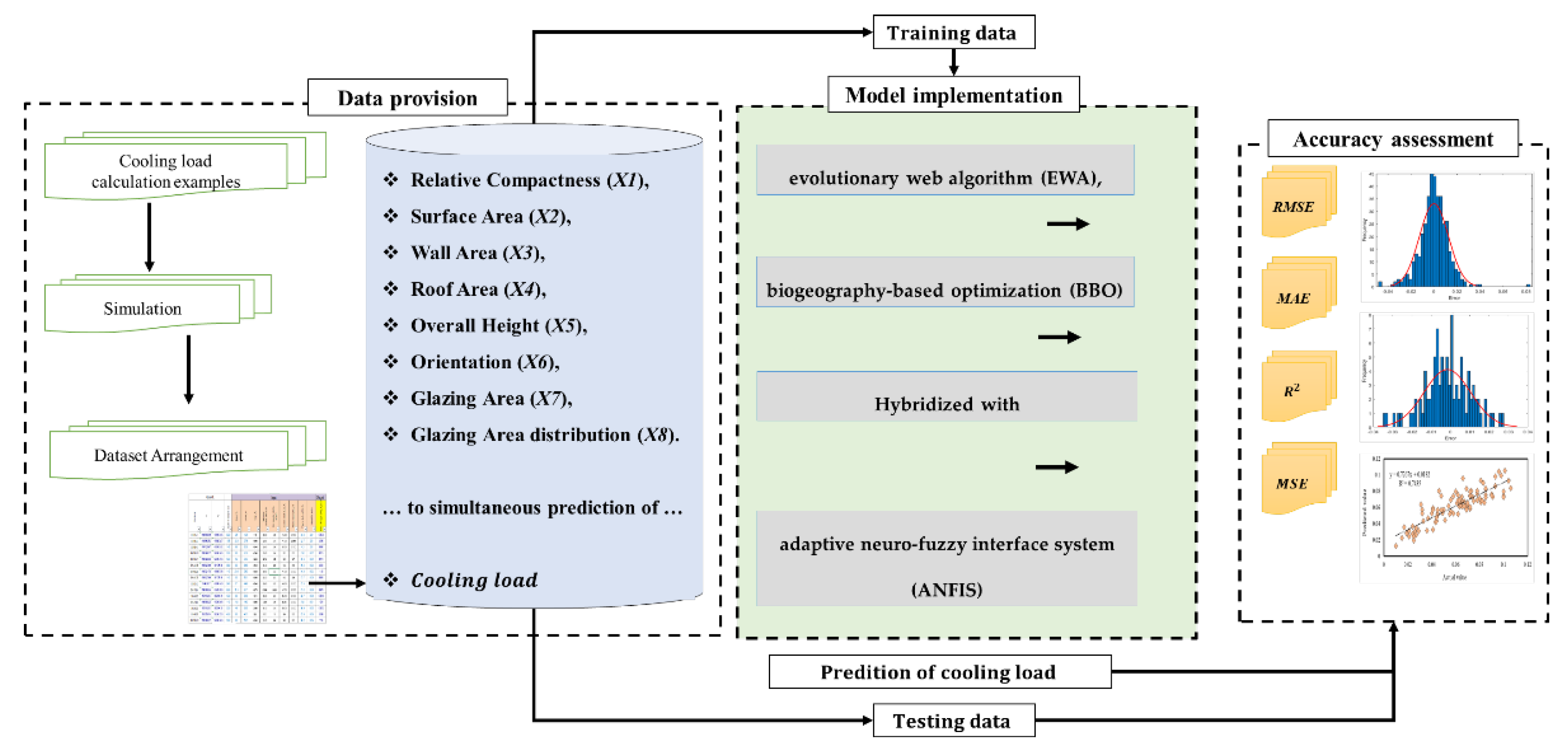
Figure 3 also illustrates the proposed hybrid model performance utilized in the current study.

4. Results and Discussion

In this study, two sophisticated computer models are employed to make predictions about the CL by taking into account the significant elements. We haphazardly picked around 80% of samples to incorporate into the training set and allocated the remaining 20% to the testing set to preserve the models’ generalizability while also preventing overfitting.

4.1. Accuracy Indicators

In order to assess the performance, three widely used performance indices, namely mean absolute error ( MAE ), coefficient of determination ( R 2 ), and root mean square error ( RMSE ), are determined [51,52,53,54]. The mathematical expressions of said indices are presented in Equations (14)–(16), along with their ideal values of 1 and 0 for R 2   and RMSE , respectively. Note that, for a perfect predictive model, the values of performance parameters should be equal to their ideal value:
RMSE = 1 U i = 1 U [ ( S i o b s e r v e d S i o b s e r v e d ) ] 2                                     14
R 2 = 1 i = 1 U S i p r e d i c t e d S i o b s e r v e d 2             i = 1 U S i o b s e r v e d S ¯ O b s e r v e d 2          
MAE = 1 U I = 1 U S i o b s e r v e d S i p r e d i c t e d                                               16
The values of CL that were actually measured and those anticipated in the environmentally friendly dwellings are represented by the variables Si observed and Si anticipate, respectively. If you want to know how many times an event has occurred, you can look up U in the formula or look up the average CL value using   s ¯ O b s e r v e d   . The enhanced dataset was used in the development of machine-learning models inside the Weka software environment. The consequences of carrying out this process are detailed in the next part.

4.2. Incorporated FIS with Optimizers

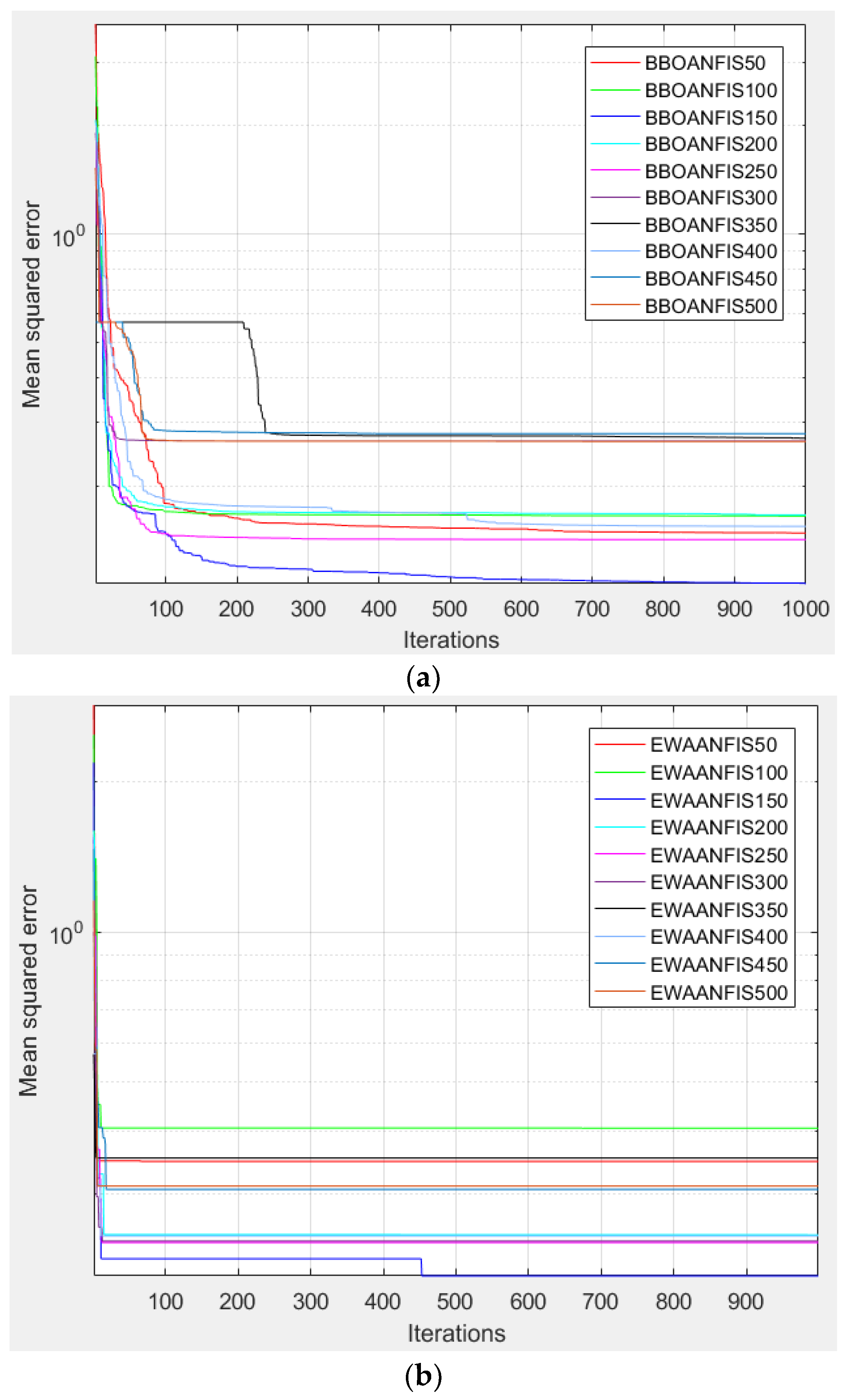
In this graph, the values of every single indicator are displayed in terms of the degree of precision obtained in relation to their respective desired values. For instance, the desired values of RMSE and R 2   are 0 and 1, correspondingly. These indicators are determined to have values of 0.10731 and 0.97776, correspondingly, for the BBO-ANFIS model when it is in the training phase in the current research. Accordingly, it is possible to deduce that the aforementioned model accomplished a precision of 89.26% (1 minus 0.10731 equals 0.89269) and 97.77% (0.97776/1 = 0.97776) with respect to the RMSE and R 2   values, respectively. During the training phase for the EWA-ANFIS model, comparable results were achieved for the   R 2   and RMSE, which came out to be 0.18682 and 0.93096, respectively (CL problem). In other words, the model attained a prediction performance of 81.31% and 93.99% when the optimum RMSE and R 2   values were 0 and 1, correspondingly. By using identical reasoning, we can also determine how accurate the other indices are. Percentage-based metrics should be transformed to decimal integers before being used. As shown in Figure 4, the MSE value is plotted against the number of iterations (1000 iterations) for each of the ten population sizes (50, 100, 150, 200, 250, 300, 350, 400, 450, and 500) that were considered in this research. The most accurate results may be attained with an RMSE that is as low as possible. According to Figure 4 and Table 2 and Table 3, the magnitude of the population of 150 produced the smallest RMSE value for BBO-ANFIS (RMSE = 0.10731 and 0.11282), but the magnitude of the population of 250 produced the smallest RMSE value for EWA-ANFIS (=0.18682 and 0.17681).
The research conducted by Zhang et al. [55] inspired the idea of ranking analysis. This method gave the model that had the greatest bargain for every indicator the highest possible rank (which was equal to the number of models being compared), and it gave the model that had the poorest value for every indicator the lowest possible rank (1), and this was conducted distinctly for the training and testing results. After that, the final score was arrived at by adding up each participant’s position in the overall standings. In the end, the total rankings achieved throughout the training and testing stages were added to get the ultimate score for every model.
The results of the performance parameters determined for every model are shown in Table 2 and Table 3, along with the models’ corresponding rankings, for the HL and CL, correspondingly. The results of these two tables make it abundantly evident that the BBO-ANFIS model is the most accurate one for predicting the CL when using a magnitude of the population of 150. In terms of the modeling of CL, EWA-ANFIS has the second-place position with a magnitude of the population of 250. The values 0.97776 and 0.97552, both associated with BBO-ANFIS, represent the highest possible R 2   score throughout the training and testing periods. Regarding EWA-ANFIS, the greatest R 2   values were 0.93096 and 0.93847, demonstrating that BBO-ANFIS provides superior performance. BBO-ANFIS had a smaller relative mean square error than EWA-ANFIS (0.17681 against 0.17682 for EWA-ANFIS), which is an important consideration when looking at the model’s overall accuracy.
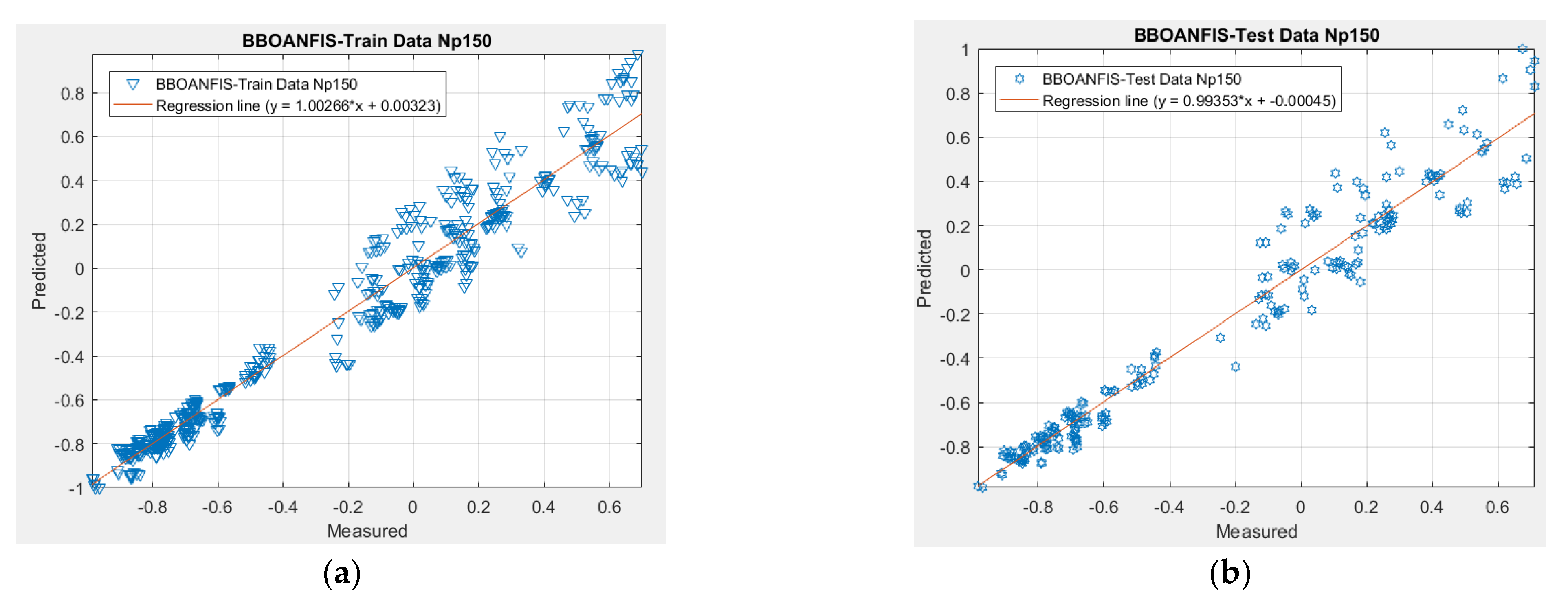
The heating and cooling demands of residential structures may now be more accurately predicted thanks to the development of two cutting-edge computer algorithms [56]. When initially training the model, the database utilized for training is called the "training dataset". The data initiated from the regression diagrams demonstrated that the BBO-ANFIS model earned the greatest R2 value, which came in at 0.97776. This corresponds to a value of 0.93096 for the EWA-ANFIS. The analysis also revealed that the majority of the estimated parameters had a very strong correlation with the experimental measurements in the testing dataset.
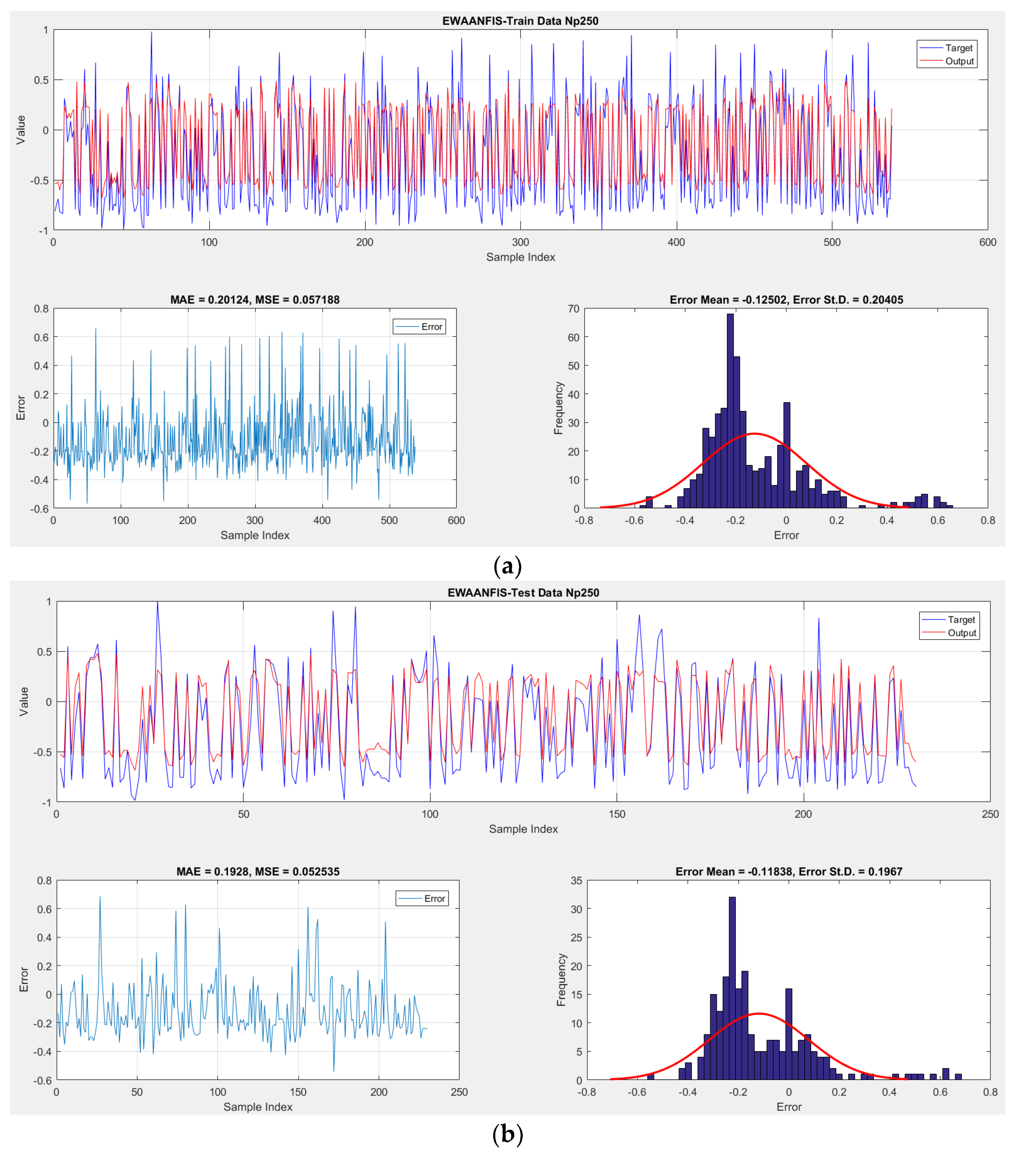
These Figure 5 and Figure 6 indicate how well the model forecasted CL from the training and testing datasets of buildings using the important factors. It is important to highlight that EWA-ANFIS came in the second position amongst some of the models that were constructed for the training dataset, behind only BBO-ANFIS.

4.3. Error Analysis

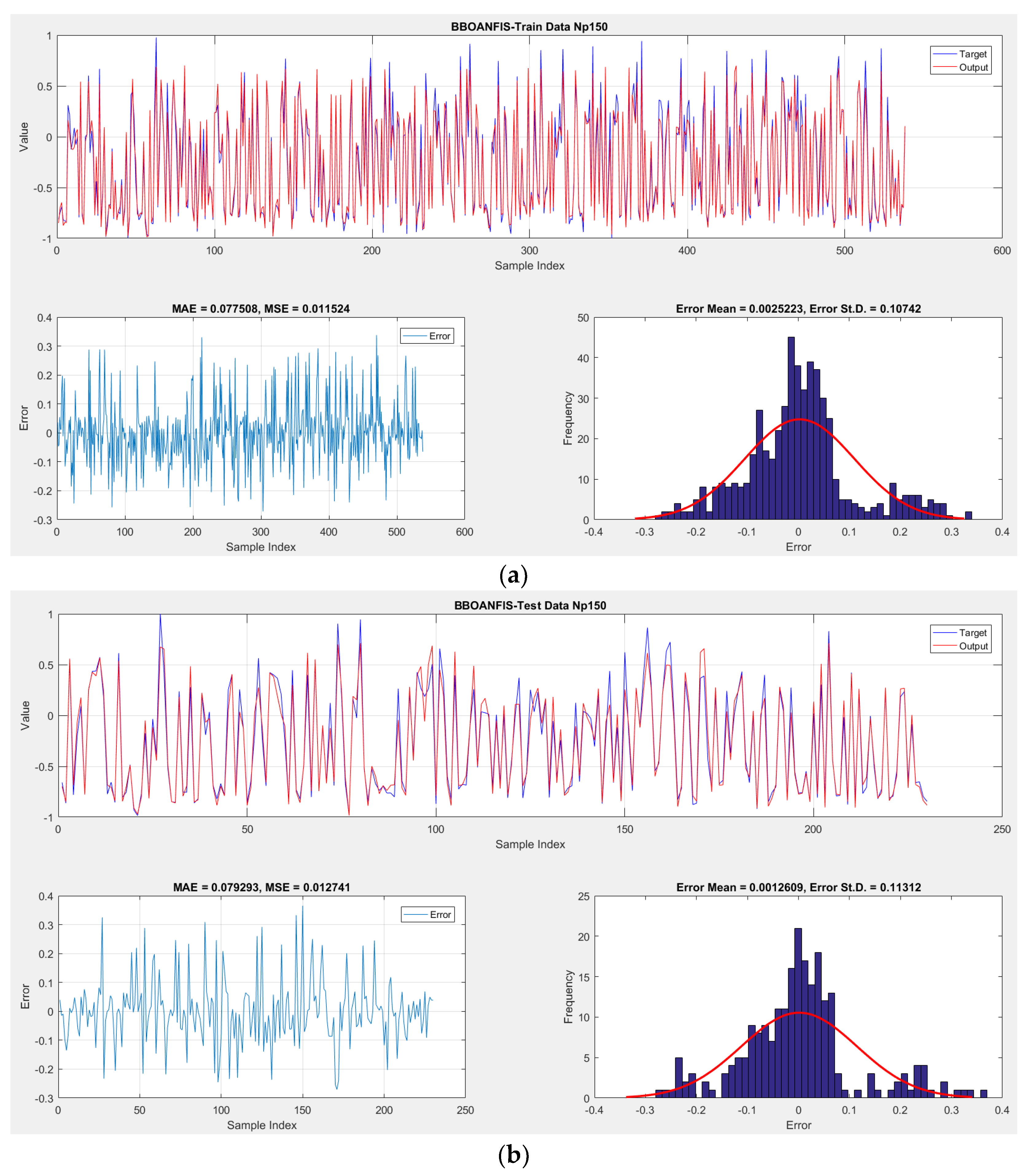
Table 2 and Table 3 demonstrate that the optimal population magnitudes for the BBO-ANFIS and EWA-ANFIS were determined to be 150 and 250, correspondingly. The occurrence of mistakes and the minimal number of mistakes in the BBO-ANFIS and EWA-ANFIS best-fitted structures are shown in Figure 7 and Figure 8, respectively. The findings initiated from the training and testing datasets showed an extremely excellent consensus between the estimated and observed values of the CL. During the training phase, MAE values of 0.077508 and 0.20124 were achieved for the BBO-ANFIS and EWA-ANFIS, in that order. Additionally, the MAE values related to the BBO-ANFIS and EWA-ANFIS models were correspondingly equal to 0.079293 and 0.1928.

4.4. Study Limitations

The outputs of the proposed soft-computing models for estimating the CL energy performance in residential buildings have been provided in the current study. The findings and explanations are also illustrated accordingly. In the first place, we described statistical findings and model different accuracy predictions, and then we got into some of the more visual aspects of the findings. Notably, MATLAB (R2016a) was used to create all hybrid computational intelligent models. On the basis of the information collected and the extensive argument offered earlier, it was demonstrated that, at all levels, the BBO-ANFIS model proved to be more efficient for modeling the energy performance of buildings.
It is worth mentioning that the proposed computational intelligent models have the potential to be used instead of traditional simulation software in order to define the CL of dwellings. These predictive models can be used in different calculations applications as a more practical way of conducting energy performance calculations [57,58]. The models developed in this work stand out for their wide applicability and inexpensive computing cost. The models described in this paper performed consistently in the testing and training stages. This shows that the models are resilient and generalizable at all levels, with no unsatisfactory values or big fluctuations in testing. Analysis and overall evaluation show that the presented models have a great deal of promise to help experts in the design process of energy-efficient megaprojects.

5. Conclusions

Within the scope of this investigation, two cutting-edge computational systems have been invented and validated for the purpose of modeling the EPB by establishing the CL of dwellings. These systems consist of EWA-ANFIS and BBO-ANFIS. In order to accomplish this goal, a dataset consisting of 768 different residential building instances was gathered and then divided into two distinct datasets: one for training (the modeling phase), which included 80% of the cases, and another for testing (the validation phase), which contained 20% of the cases. RMSE and R 2   were two indicators used to assess the models’ accuracy and predictability in weather forecasting. Experiments have shown that the non-linear interactions between CL and its influencing factors can be accurately modeled using established models. According to the findings, BBO-ANFIS demonstrated superior performance when compared to the other model. In addition, the results showed that BBO-ANFIS was the most powerful forecasting model out of the two models that were suggested in terms of achieving the lowest value of root mean square error (RMSE) and the greatest value of correlation coefficient ( R 2   ) (RMSE = 0.10731 and 0.11282 and R 2   = 0.97776 and 0.97552 for the training and testing phases, correspondingly). In addition, the EWA-ANFIS demonstrated RMSE values of 0.18682 and 0.17681 and R 2   values of 0.93096 and 0.93874 during the training and testing phases, in that order. Since only three methods were included in this work (BBO, EWA, and ANFIS), other methods will also be included in future work, taking into account other possible input variables by the addition of thermal insulation. To conclude, this study has proven that ANN is a powerful tool and will be useful for predicting the CL in residential buildings.

Author Contributions

H.M.: methodology, software; B.L.V.: data curation, revision preparation. All authors have read and agreed to the published version of the manuscript.

Funding

This research received no external funding.

Data Availability Statement

The data are available based on the reader’s request.

Conflicts of Interest

The authors declare no conflict of interest.

References

  1. Yu, Z.; Haghighat, F.; Fung, B.C.; Yoshino, H. A decision tree method for building energy demand modeling. Energy Build. 2010, 42, 1637–1646. [Google Scholar] [CrossRef] [Green Version]
  2. Tsanas, A.; Xifara, A. Accurate quantitative estimation of energy performance of residential buildings using statistical machine learning tools. Energy Build. 2012, 49, 560–567. [Google Scholar] [CrossRef]
  3. Ali, A.; Zhang, C.; Bibi, T.; Zhu, L.; Cao, L.; Li, C.; Hsiao, P.-C. Investigation of five different low-cost locally available isolation layer materials used in sliding base isolation systems. Soil Dyn. Earthq. Eng. 2022, 154, 107127. [Google Scholar] [CrossRef]
  4. Pérez-Lombard, L.; Ortiz, J.; Pout, C. A review on buildings energy consumption information. Energy Build. 2008, 40, 394–398. [Google Scholar] [CrossRef]
  5. Cai, W.; Wu, Y.; Zhong, Y.; Ren, H. China building energy consumption: Situation, challenges and corresponding measures. Energy Policy 2009, 37, 2054–2059. [Google Scholar] [CrossRef]
  6. Zhang, Y.; Shi, X.; Zhang, H.; Cao, Y.; Terzija, V. Review on deep learning applications in frequency analysis and control of modern power system. Int. J. Electr. Power Energy Syst. 2022, 136, 107744. [Google Scholar] [CrossRef]
  7. Platt, G.; Li, J.; Li, R.; Poulton, G.; James, G.; Wall, J. Adaptive HVAC zone modeling for sustainable buildings. Energy Build. 2010, 42, 412–421. [Google Scholar] [CrossRef]
  8. Yao, R.; Li, B.; Steemers, K. Energy policy and standard for built environment in China. Renew. Energy 2005, 30, 1973–1988. [Google Scholar] [CrossRef]
  9. Huang, H.; Huang, M.; Zhang, W.; Yang, S. Experimental study of predamaged columns strengthened by HPFL and BSP under combined load cases. Struct. Infrastruct. Eng. 2021, 17, 1210–1227. [Google Scholar] [CrossRef]
  10. Yezioro, A.; Dong, B.; Leite, F. An applied artificial intelligence approach towards assessing building performance simulation tools. Energy Build. 2008, 40, 612–620. [Google Scholar] [CrossRef]
  11. Crawley, D.B.; Hand, J.W.; Kummert, M.; Griffith, B.T. Contrasting the capabilities of building energy performance simulation programs. Build. Environ. 2008, 43, 661–673. [Google Scholar] [CrossRef] [Green Version]
  12. Li, H.; Hou, K.; Xu, X.; Jia, H.; Zhu, L.; Mu, Y. Probabilistic energy flow calculation for regional integrated energy system considering cross-system failures. Appl. Energy 2022, 308, 118326. [Google Scholar] [CrossRef]
  13. Seyedzadeh, S.; Rahimian, F.P.; Rastogi, P.; Glesk, I. Tuning machine learning models for prediction of building energy loads. Sustain. Cities Soc. 2019, 47, 101484. [Google Scholar] [CrossRef]
  14. Xie, X.; Sun, Y. A piecewise probabilistic harmonic power flow approach in unbalanced residential distribution systems. Int. J. Electr. Power Energy Syst. 2022, 141, 108114. [Google Scholar] [CrossRef]
  15. Zhao, M.; Zhou, Y.; Li, X.; Zhou, C.; Cheng, W.; Li, M.; Huang, K. Building a series of consistent night-time light data (1992–2018) in Southeast Asia by integrating DMSP-OLS and NPP-VIIRS. IEEE Trans. Geosci. Remote Sens. 2019, 58, 1843–1856. [Google Scholar] [CrossRef]
  16. Zhao, H.-x.; Magoulès, F. A review on the prediction of building energy consumption. Renew. Sustain. Energy Rev. 2012, 16, 3586–3592. [Google Scholar] [CrossRef]
  17. Zhao, Y.; Foong, L.K. Predicting Electrical Power Output of Combined Cycle Power Plants Using a Novel Artificial Neural Network Optimized by Electrostatic Discharge Algorithm. Measurement 2022, 198, 111405. [Google Scholar] [CrossRef]
  18. Foong, L.K.; Zhao, Y.; Bai, C.; Xu, C. Efficient metaheuristic-retrofitted techniques for concrete slump simulation. Smart Struct. Syst. Int. J. 2021, 27, 745–759. [Google Scholar]
  19. Lu, S.; Ban, Y.; Zhang, X.; Yang, B.; Yin, L.; Liu, S.; Zheng, W. Adaptive control of time delay teleoperation system with uncertain dynamics. Front. Neurorobot. 2022, 16, 928863. [Google Scholar] [CrossRef]
  20. Zhao, M.; Zhou, Y.; Li, X.; Cheng, W.; Zhou, C.; Ma, T.; Li, M.; Huang, K. Mapping urban dynamics (1992–2018) in Southeast Asia using consistent nighttime light data from DMSP and VIIRS. Remote Sens. Environ. 2020, 248, 111980. [Google Scholar] [CrossRef]
  21. Crawley, D.B.; Lawrie, L.K.; Winkelmann, F.C.; Buhl, W.F.; Huang, Y.J.; Pedersen, C.O.; Strand, R.K.; Liesen, R.J.; Fisher, D.E.; Witte, M.J. EnergyPlus: Creating a new-generation building energy simulation program. Energy Build. 2001, 33, 319–331. [Google Scholar] [CrossRef]
  22. Citherlet, S. Towards the Holistic Assessment of Building Performance Based on an Integrated Simulation Approach. 2001. Available online: https://www.semanticscholar.org/paper/Towards-the-holistic-assessment-of-building-based-Citherlet/e4d8bbb0ad26827f539df78bc32749bf0e402d88 (accessed on 27 August 2022).
  23. Duanmu, L.; Wang, Z.; Zhai, Z.J.; Li, X. A simplified method to predict hourly building cooling load for urban energy planning. Energy Build. 2013, 58, 281–291. [Google Scholar] [CrossRef]
  24. Husaunndee, A.; Lahrech, R.; Vaezi-Nejad, H.; Visier, J. SIMBAD: A simulation toolbox for the design and test of HVAC control systems. In Proceedings of the 5th International IBPSA Conference, Prague, Czech Republic, 8–10 September 1997; pp. 269–276. [Google Scholar]
  25. Murray, M.C.; Finlayson, N.; Kummert, M.; Macbeth, J. Live Energy TRNSYS–TRNSYS Simulation within Google SketchUp. In Proceedings of the Eleventh International IBPSA Conference, Glasgow, Scotland, 27–30 July 2009; pp. 1389–1396. [Google Scholar]
  26. Hafner, B.; Plettner, J.; Wemhöner, C.; Wenzel, T. CARNOT Blockset-User’s Guide; Solar-Institut Jülich der FH Aachen: Aachen, Germany, 1999. [Google Scholar]
  27. Yan, B.; Ma, C.; Zhao, Y.; Hu, N.; Guo, L. Geometrically Enabled Soft Electroactuators via Laser Cutting. Adv. Eng. Mater. 2019, 21, 1900664. [Google Scholar] [CrossRef]
  28. Gong, X.; Wang, L.; Mou, Y.; Wang, H.; Wei, X.; Zheng, W.; Yin, L. Improved Four-channel PBTDPA control strategy using force feedback bilateral teleoperation system. Int. J. Control. Autom. Syst. 2022, 20, 1002–1017. [Google Scholar] [CrossRef]
  29. Wang, J.; Tian, J.; Zhang, X.; Yang, B.; Liu, S.; Yin, L.; Zheng, W. Control of Time Delay Force Feedback Teleoperation System with Finite Time Convergence. Front. Neurorobot. 2022, 16, 877069. [Google Scholar] [CrossRef]
  30. Kalogirou, S.A.; Neocleous, C.; Schizas, C. Building heating load estimation using artificial neural networks. In Proceedings of the 17th International Conference on Parallel Architectures and Compilation Techniques, San Francisco, CA, USA, 11–15 November 1997; p. 14. [Google Scholar]
  31. Xie, X.; Chen, D. Data-driven dynamic harmonic model for modern household appliances. Appl. Energy 2022, 312, 118759. [Google Scholar] [CrossRef]
  32. Catalina, T.; Virgone, J.; Blanco, E. Development and validation of regression models to predict monthly heating demand for residential buildings. Energy Build. 2008, 40, 1825–1832. [Google Scholar] [CrossRef]
  33. Dong, B.; Cao, C.; Lee, S.E. Applying support vector machines to predict building energy consumption in tropical region. Energy Build. 2005, 37, 545–553. [Google Scholar] [CrossRef]
  34. Zhang, J.; Haghighat, F. Development of Artificial Neural Network based heat convection algorithm for thermal simulation of large rectangular cross-sectional area Earth-to-Air Heat Exchangers. Energy Build. 2010, 42, 435–440. [Google Scholar] [CrossRef]
  35. Deb, C.; Eang, L.S.; Yang, J.; Santamouris, M. Forecasting diurnal cooling energy load for institutional buildings using Artificial Neural Networks. Energy Build. 2016, 121, 284–297. [Google Scholar] [CrossRef]
  36. Mena, R.; Rodríguez, F.; Castilla, M.; Arahal, M.R. A prediction model based on neural networks for the energy consumption of a bioclimatic building. Energy Build. 2014, 82, 142–155. [Google Scholar] [CrossRef]
  37. Platon, R.; Dehkordi, V.R.; Martel, J. Hourly prediction of a building’s electricity consumption using case-based reasoning, artificial neural networks and principal component analysis. Energy Build. 2015, 92, 10–18. [Google Scholar] [CrossRef]
  38. Zhao, Y.; Moayedi, H.; Bahiraei, M.; Foong, L.K. Employing TLBO and SCE for optimal prediction of the compressive strength of concrete. Smart Struct. Syst. 2020, 26, 753–763. [Google Scholar]
  39. Li, K.; Hu, C.; Liu, G.; Xue, W. Building’s electricity consumption prediction using optimized artificial neural networks and principal component analysis. Energy Build. 2015, 108, 106–113. [Google Scholar] [CrossRef]
  40. Hong, S.-M.; Paterson, G.; Mumovic, D.; Steadman, P. Improved benchmarking comparability for energy consumption in schools. Build. Res. Inf. 2014, 42, 47–61. [Google Scholar] [CrossRef]
  41. Khayatian, F.; Sarto, L. Application of neural networks for evaluating energy performance certificates of residential buildings. Energy Build. 2016, 125, 45–54. [Google Scholar] [CrossRef]
  42. Zhao, Y.; Joseph, A.J.J.M.; Zhang, Z.; Ma, C.; Gul, D.; Schellenberg, A.; Hu, N. Deterministic snap-through buckling and energy trapping in axially-loaded notched strips for compliant building blocks. Smart Mater. Struct. 2020, 29, 02LT03. [Google Scholar] [CrossRef]
  43. Samui, P.; Kim, D.; Viswanathan, R. Spatial variability of rock depth using adaptive neuro-fuzzy inference system (ANFIS) and multivariate adaptive regression spline (MARS). Environ. Earth Sci. 2015, 73, 4265–4272. [Google Scholar] [CrossRef]
  44. Jang, J.-S. ANFIS: Adaptive-network-based fuzzy inference system. IEEE Trans. Syst. Man Cybern. 1993, 23, 665–685. [Google Scholar] [CrossRef]
  45. Zhao, Y.; Wang, Z. Subset simulation with adaptable intermediate failure probability for robust reliability analysis: An unsupervised learning-based approach. Struct. Multidiscip. Optim. 2022, 65, 172. [Google Scholar] [CrossRef]
  46. Barak, S.; Sadegh, S.S. Forecasting energy consumption using ensemble ARIMA–ANFIS hybrid algorithm. Int. J. Electr. Power Energy Syst. 2016, 82, 92–104. [Google Scholar] [CrossRef] [Green Version]
  47. Zhao, Y.; Hu, H.; Bai, L.; Tang, M.; Chen, H.; Su, D. Fragility analyses of bridge structures using the logarithmic piecewise function-based probabilistic seismic demand model. Sustainability 2021, 13, 7814. [Google Scholar] [CrossRef]
  48. Simon, D. Biogeography-based optimization. IEEE Trans. Evol. Comput. 2008, 12, 702–713. [Google Scholar] [CrossRef] [Green Version]
  49. Bhattacharya, A.; Chattopadhyay, P.K. Biogeography-based optimization for different economic load dispatch problems. IEEE Trans. Power Syst. 2009, 25, 1064–1077. [Google Scholar] [CrossRef]
  50. Wang, G.-G.; Deb, S.; Coelho, L.D.S. Earthworm optimisation algorithm: A bio-inspired metaheuristic algorithm for global optimisation problems. Int. J. Bio-Inspired Comput. 2018, 12, 1–22. [Google Scholar] [CrossRef]
  51. Samui, P.; Kumar, R.; Yadav, U.; Kumari, S.; Bui, D.T. Reliability analysis of slope safety factor by using GPR and GP. Geotech. Geol. Eng. 2019, 37, 2245–2254. [Google Scholar] [CrossRef]
  52. Ray, R.; Kumar, D.; Samui, P.; Roy, L.B.; Goh, A.; Zhang, W. Application of soft computing techniques for shallow foundation reliability in geotechnical engineering. Geosci. Front. 2021, 12, 375–383. [Google Scholar] [CrossRef]
  53. Kumar, M.; Samui, P. Reliability analysis of pile foundation using ELM and MARS. Geotech. Geol. Eng. 2019, 37, 3447–3457. [Google Scholar] [CrossRef]
  54. Kardani, M.N.; Baghban, A.; Hamzehie, M.E.; Baghban, M. Phase behavior modeling of asphaltene precipitation utilizing RBF-ANN approach. Pet. Sci. Technol. 2019, 37, 1861–1867. [Google Scholar] [CrossRef]
  55. Zhang, H.; Zhou, J.; Jahed Armaghani, D.; Tahir, M.; Pham, B.T.; Huynh, V.V. A combination of feature selection and random forest techniques to solve a problem related to blast-induced ground vibration. Appl. Sci. 2020, 10, 869. [Google Scholar] [CrossRef] [Green Version]
  56. Zhao, Y.; Zhong, X.; Foong, L.K. Predicting the splitting tensile strength of concrete using an equilibrium optimization model. Steel Compos. Struct. Int. J. 2021, 39, 81–93. [Google Scholar]
  57. Zhao, Y.; Hu, H.; Song, C.; Wang, Z. Predicting compressive strength of manufactured-sand concrete using conventional and metaheuristic-tuned artificial neural network. Measurement 2022, 194, 110993. [Google Scholar] [CrossRef]
  58. Zhao, Y.; Yan, Q.; Yang, Z.; Yu, X.; Jia, B. A novel artificial bee colony algorithm for structural damage detection. Adv. Civ. Eng. 2020, 6, 3743089. [Google Scholar] [CrossRef]
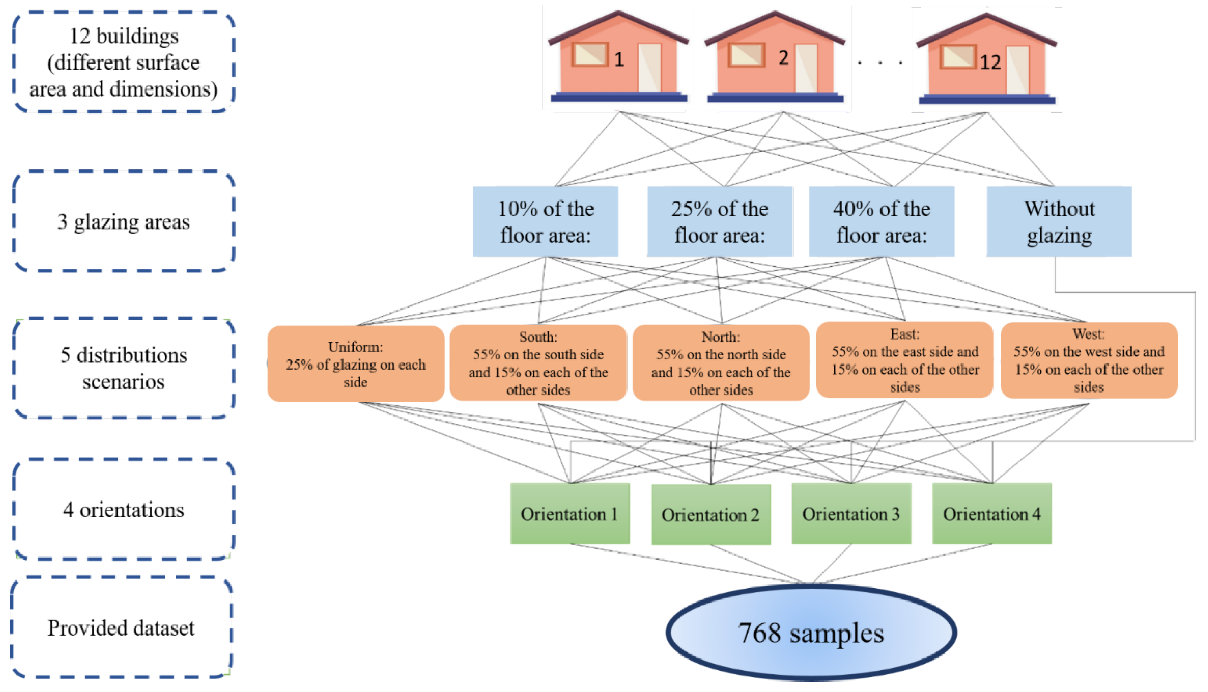
Figure 1. Graphical view of data preparation.
Energies 15 07323 g001
Figure 2. Schematic of an ANFIS Structure.
Energies 15 07323 g002
Figure 3. Proposed hybrid model performance.
Energies 15 07323 g003
Figure 4. Variation of mean squared error versus iterations for the (a) BBOANFIS, (b) EWA-ANFIS.
Energies 15 07323 g004
Figure 5. The accuracy of training and testing dataset performance of BBO−ANFIS in the best-fit optimization structure: (a) BBO−ANFIS train Np = 150; (b) BBO−ANFIS test Np = 150.
Energies 15 07323 g005
Figure 6. The accuracy of training and testing dataset performance of EWA−ANFIS in the best-fit optimization structure: (a) EWA−ANFIS train Np = 250; (b) EWA−ANFIS test Np = 250.
Energies 15 07323 g006
Figure 7. Frequency and minimum value of errors in BBOANFIS best-fit structure: (a) training dataset; (b) testing dataset.
Energies 15 07323 g007
Figure 8. Frequency and minimum value of errors in EWAANFIS best-fit structure: (a) training dataset; (b) testing dataset.
Energies 15 07323 g008
Table 1. Statistical summary of the input and output variables.
Input VariablesCount Mean MinMax Std.
Relative Compactness (-)7680.7640.620.980.105
Surface Area (m2)768671.7514.5808.588.08
Wall Area (m2)768318.5245416.543.62
Roof Area (m2)768176.6110.25220.545.16
Overall Height (m)7685.253.571.751
Orientation (-)7683.5251.118
Glazing Area (m2)7680.234040.133
Glazing Area Distribution7682.812051.55
Output VariablesCount Mean MinMax Std.
CL (kwh/m2)76824.5810.948.039.513
Table 2. The network results for the BBOANFIS for different swarm sizes.
Swarm SizeTraining DatasetTesting DatasetScoringTotal ScoreRank
RMSER2RMSER2TrainingTesting
500.14820.957140.138770.962738888323
1000.165360.946350.154910.953336677264
1500.107310.977760.112820.9755210101010401
2000.166440.945620.159830.950245555206
2500.142290.960560.138310.962989999362
3000.228120.895120.215260.907723333128
3500.237620.885630.222980.90061222289
4000.154790.953150.155040.953247766264
4500.250890.871550.236610.88731111410
5000.225090.898050.209590.912754444167
Table 3. The network results for the EWAANFIS for different swarm sizes.
Swarm SizeTraining DatasetTesting DatasetScoringTotal ScoreRank
RMSER2RMSER2TrainingTesting
500.304170.804140.302310.807951111410
1000.245490.87740.237440.886464444167
1500.19360.925660.210730.911759988342
2000.240250.882930.233950.889986666245
2500.186820.930960.176810.9387410101010401
3000.230890.892410.22140.90217777284
3500.275110.843170.274160.84525222289
4000.222590.900430.2090.913268899342
4500.262630.858240.261120.860783333128
5000.24260.880460.234570.889365555206
Publisher’s Note: MDPI stays neutral with regard to jurisdictional claims in published maps and institutional affiliations.