Article

A Coal Seam Thickness Prediction Model Based on CPSAC and WOA–LS-SVM: A Case Study on the ZJ Mine in the Huainan Coalfield

1
School of Earth and Environment, Anhui University of Science and Technology, Huainan 232001, China
2
Geophysical Prospecting Research Institute, CNACG, Zhuozhou 072750, China
*
Author to whom correspondence should be addressed.
Energies 2022, 15(19), 7324; https://doi.org/10.3390/en15197324
Submission received: 6 September 2022 / Revised: 1 October 2022 / Accepted: 3 October 2022 / Published: 5 October 2022

Abstract

:
The precise prediction of coal seam thickness in operating mines is crucial for the construction of transparent mines. Geological borehole data or a small amount of seismic information is frequently used in traditional coal seam thickness prediction methods; however, these methods have poor precision. In this study, we introduced a model for predicting coal seam thickness based on the comprehensive preference for seismic attribute combination (CPSAC) and the least squares support vector machine (LS-SVM) optimized by the whale optimization algorithm (WOA). We used the CPSAC to modify the mass disturbed data in the seismic attribute data to predict the coal seam thickness. To achieve this the sample size was reduced by optimizing the seismic attribute combinations, and the modified attribute data was entered into the LS-SVM., Furthermore, to create an accurate prediction model for coal thickness, we employed the WOA to determine the optimal penalty coefficient and kernel coefficient of the LS-SVM. An empirical case study was conducted in the northeast mining area of the ZJ mine in the Huainan coalfield. The coal thickness of two mining faces in this research area were estimated and compared, demonstrating the proposed method’s high prediction accuracy. The proposed method has guiding implications for developing an accurate mining geological model and facilitating the accurate use of coal resources.

1. Introduction

Coal seam thickness is an important parameter for identifying coal resource reserves; it directly affects the design and construction of mines and restricts the design of the working face, selection of mining supports, and gas management. Furthermore, coal seam thickness has important guiding significance for surface deformation monitoring, environmental treatment, and comprehensive utilization of closed pit mine resources [1,2,3,4]. Consequently, accurate coal seam thickness prediction in operating mines has become an important area of study for constructing transparent mines. However, the coal seam thickness determined by direct interpolation between boreholes and extrapolation is inaccurate in terms of the actual thickness based on the conventional prediction approach [5].
Three-dimensional (3D) seismic data have the characteristics of dense sampling and horizontal continuity; consequently, they can effectively reflect the distribution and structural development of geological coal seams in combination with the calibration of sparse geological borehole data. Therefore, the use of 3D seismic information to predict coal seam thickness has attracted considerable attention and has gradually developed into a mainstream technology for precisely predicting coal seam thickness. In recent decades, studies have indicated that seismic attributes respond to the geometric, kinematic, kinetic, and statistical characteristics of seismic waveforms. Moreover, by extracting multiple attribute parameters and using multiple mathematical statistical methods and intelligent algorithms to synthesize different attributes for analysis and prediction, the thickness of thin coal seams can be quantitatively predicted. Therefore, the method of coal thickness prediction using seismic multi-attributes has been widely used and studied in depth.
Ricker [6], Widess [7], Ruter and Schepers [8], and Koefoed and De Voogd [9] examined the relationship between the thickness of thin areas and seismic wave wavelength and amplitude, which provided the theoretical foundation for subsequent studies. Cheng et al. [10], Dong [11], Suo et al. [12] and Meng [13] performed in-depth studies on the formation mechanism of coal seam reflection waves, the response laws of attributes (e.g., seismic wave amplitude and frequency under the conditions of coal thickness change), and quantitative interpretation methods of coal seam thickness as per the designed seismic geological model of coal seams. Liu et al. [14], Liu et al. [15], and Peng et al. [16] proposed coal thickness interpretation methods such as the spectral moment method, trace integration method, and the seismic wave impedance inversion method constrained by well logs, based on thin-layer theory and the formation mechanism of coal seam reflection waves and achieved favorable application results.
The deep integration of seismic multi-attribute and mathematical methods marked a new stage in coal thickness prediction research. Artificial neural networks, fuzzy neural networks, deep belief networks, extreme value learning machines, and support vector machines (SVMs) have been applied to studies on coal thickness prediction [17,18,19,20,21,22,23,24,25]. However, these methods have not been extensively applied in the coal mining industry because of limitations in learning speed and modeling capacity. Furthermore, to eliminate the mutual interference between attributes, mathematical methods for dimension reduction, such as correlation analysis (CA), principal component analysis (PCA), and kernel principal component analysis (KPCA), are commonly used for seismic attribute approximation [26,27]. Consequently, to improve the prediction accuracy, Chen et al. [28] and Fan et al. [29] proposed using the particle swarm optimization algorithm for the parameter optimization of mathematical models
Although the abovementioned studies proposed prediction methods for solving the seismic multi-attribute coal thickness prediction problem and partially achieved precise coal thickness prediction, they had multiple limitations. First, the selection of seismic attribute combinations and dimensions depended only on the initial geological exploration borehole data, which was not dynamically adjusted using the increased coal thickness sample data during the production stage of the mine. The method thus failed to make a comparative selection based on the confirmation of the model prediction results. Second, neural-network-like methods suffer from complex network structures, overfitting, and local traps when solving small-sample problems. Furthermore, the selection of the kernel function and penalty parameters of SVM considerably affects the classification and prediction accuracy of the model, and it is necessary to continuously optimize the prediction model using advanced intelligent algorithms.
To achieve precise prediction of coal seam thickness in operating mines, we propose a prediction model in operating mines based on the comprehensive preference for seismic attribute combination (CPSAC) and the whale-optimization-algorithm-optimized least squares support vector machine (WOA–LS-SVM) in this study.

2. The CPSAC

Seismic attribute parameters are not independent; certain attributes contain similar or identical information, whereas others are unrelated and do not contain identical information. All seismic attributes have different sensitivities to the predicted objects. For predicting coal seam thickness, a large number of seismic attribute parameters does not lead to better performance. If seismic attributes are involved in prediction model training without identification and many of these attributes are blindly used for coal thickness prediction, the time and space complexity of the prediction algorithm will increase. Consequently, the accuracy and reliability of the prediction will be adversely affected. Therefore, it is necessary to select multiple seismic attributes, study the correlation between seismic attribute parameters and their correlation with coal thickness, and determine the combination of seismic attribute parameters that can best reflect the characteristics of coal thickness change and are independent of each other. These seismic attributes can then be used as parameters for constructing a coal thickness prediction model.
The conventional seismic attribute preference primarily depends on dimension-reduction mathematical methods such as CA and PCA; however, this approach has several limitations. First, the nonlinear relationships among seismic attributes are not considered, and the method of processing linear correlation data is used to approximate seismic attributes. Second, the selection of seismic attribute combinations and dimensions depends on only a small amount of geological exploration borehole data and cannot be dynamically adjusted with an increase in coal thickness sample data in the production stage of mines. Therefore, in this study we propose a comprehensive optimization framework for a seismic attribute combination based on KPCA, a seismic attribute classification, and comparative validation in different stages (as illustrated in Figure 1) to address the above problems. The main implementation steps are provided in Appendix A.

3. The WOA–LS-SVM Coal Seam Thickness Prediction Model

3.1. The Whale Optimization Algorithm (WOA)

There exist multiple intelligent algorithms such as the bat algorithm, artificial bee colony algorithm, wolf optimization algorithm, and bird swarm algorithm [30,31,32,33]. The results of using different intelligent algorithms to solve optimization problems in different fields also differ. In this study, we propose to use a new population intelligence optimization algorithm, the WOA, which is concise, easy to implement, and has the advantages of more relaxed requirements for the objective function and lower parameter control.
Mirjalili and Lewis [34], Kaur and Arora [35], and Mafarja and Mirjalili [36] proposed the WOA by analyzing and studying the daily foraging behavior of whales. The algorithm achieved optimization by simulating the unique bubble-net foraging strategy of whales. The three stages of the optimization algorithm are described in Section 3.1.1, Section 3.1.2 and Section 3.1.3.

3.1.1. Surrounding the Prey

Because the optimal problem solution is not previously known, the WOA continuously updates its position during the search process by randomly assuming the position in which the individual is located. The mathematical model is as follows:
D = C X * t X t
X t + 1 = X * t A D
where D is the distance between the whale and the target prey, t is the number of current iterations, X is the current individual coordinate vector, and X* is the current location optimal solution vector. Note that both A and C are coefficient vectors with the following equations:
A = 2 a r 1 a
C = 2 r 2
where a is the convergence factor, which linearly decreases from 2 to 0 with the number of iterations, and r1 and r2 are random numbers generated from 0 to 1.

3.1.2. Bubble-Net Attacks

Whales usually feed by bubble-net attacks. To interpret this foraging behavior from a mathematical viewpoint, two methods have been designed: the shrinkage envelope mechanism and the spiral update position. The shrinkage envelope refers to the process of approaching the selected individuals by reducing a in Equation (3). The current individual position vector (X, Y) shrinks to the optimal position vector (X*, Y*). The spiral update position primarily simulates the path of the whale population approaching the prey. The numerical expression of this method is based on the distance between the current position vector (X, Y) and the current optimal position (X*, Y*).

3.1.3. Random Search

In the abovementioned bubble-net attacks, the whales randomly search for prey with coefficient A > 1, indicating that the whales swim outside the constricted envelope at which time individual whales randomly search out each other’s positions. The WOA randomly initializes a set of solutions and updates its position as per the optimal solution during each iteration. The convergence factor considerably affects the efficiency of the algorithm in identifying the optimal solution. Although the convergence factor can improve the global search, the search speed is slow. A smaller convergence factor can increase the efficiency of a local search. Nevertheless, it is easy to fall into the local optimum, leading to poor convergence accuracy and thus an inability to efficiently find the optimal solution.

3.2. The Least Squares Support Vector Machine (LS-SVM)

In 2002, Suykens et al. [37] proposed the LS-SVM, an extension of SVM. The LS-SVM can develop a fitted model with high accuracy based on smaller datasets, with the advantages of high generalization ability, fast operation speed, and relatively simple operation. Therefore, the LS-SVM is popular in prediction, evaluation, and classification, and its linear regression function can be expressed as follows:
y x = ω g φ x + b
where y is the input variable, ω is the weight vector, φ(x) is the mapping function, and b is the bias vector.
To reduce the structural risk, the LS-SVM uses an optimization approach to solve the relevant parameters:
min ω , b , e J ω , e = 1 2 ω T ω + 1 2 γ k = 1 N e k 2
y k = ω T φ x k + b + e k , k = 1 , , N
where γ is the penalty coefficient, ek is the introduced fitting error, and b is the threshold value. To solve this limitation, the LS-SVM introduces Lagrange multipliers αk (non-negative) and then develops Lagrange functions that transform the optimization problem into the following:
L ω , b , e , α = J ω , e k = 1 N α k ω T φ x k + b + e k y k
After introducing the kernel function, eliminating ω and ek, the LS-SVM prediction model can be expressed as follows:
y x = k = 1 N α k K x , x k + b

3.3. The Coal Thickness Prediction Model

The LS-SVM is affected by the penalty factor γ and kernel function parameter δ2 and in turn affects the prediction accuracy and prediction results. In this study, the WOA is applied to the LS-SVM for identifying the optimal parameters γ and δ2. The optimal position of the whale is used as the two parameter values of the LS-SVM. The advantages of strong global search ability and fast convergence of the WOA are used to compensate for the randomness of the LS-SVM in selecting the parameters. Therefore, the algorithm is not easily trapped in the local optimum and thus achieves improved generalization ability. Furthermore, the original parameters of the WOA are optimized to accelerate the convergence speed to help obtain the optimal parameters of the LS-SVM and improve its coal thickness prediction accuracy. Appendix B shows the pseudocode of the WOA.
Based on the preprocessing of the existing coal thickness and seismic multi-attribute data, the range of optimization parameters is determined. The output data are coal thickness Y(t) at the prediction point; and the LS-SVM is trained with randomly given training data, (X(t), Y(t)), to optimize the parameters as per the fitness function and iterate continuously. It then obtains the optimal parameters to develop the WOA–LS-SVM coal thickness prediction model. The primary process is illustrated in Figure 2 and described in detail in Appendix C.

4. Application Cases

4.1. Overview of the Study Area

The northeast mining area of the ZJ mine in the Huainan coalfield, located in the north-central part of Anhui Province, Eastern China, where the surface belongs to the Huaihe alluvial plain, was selected as the study area. The topography was flat, with a ground elevation of +22.4 to +23.4 m and the low hill of Minglong in the northeast. The area had the characteristics of a Carboniferous-Permian coalfield underlain by a giant thick loose layer. The coal-bearing strata were the Upper Carboniferous Taiyuan (C3t), Lower Permian Shanxi (P1S) and Lower Shibox (P1XS), and Upper Permian Upper Shibox (P2SS), with a total thickness of about ~900 m, containing ~40 coal seams and 13 recoverable coal seams, of which the 13-1 coal seam was the uppermost main mining seam, having a general coal thickness of 3–4.8 m, averaging 4 m with a simple structure.
The study area exhibited favorable shallow seismic geological conditions, a thick primary mineable coal seam, and large physical differences between top and bottom plates. The physical differences between the 13-1 coal seam and the surrounding rocks were obvious; furthermore, the formed reflected wave group had strong energy, high stability, and good continuity. In 2007, the area was surveyed via a conventional 3D seismic survey in the mining area using a bundle of eight lines and eight shots, a bilateral symmetric receiving observation system with complete coverage of 24 times, a receiving channel distance of 20 m, a receiving line distance of 40 m, and a CDP grid specification of 10 m × 10 m.
The study area was approximately rectangular in plan having a length of ~2 km from north to south and a width of ~1.2 km from east to west, thus covering an area of 2.45 km2. As shown in Figure 3, a total of 13 geological boreholes and 16 surface gas drilling wells were drilled in the exploration stage. In the mining area, there were three coal mining faces of the 13-1 coal seam, two of which had been mined and one of which was yet to be mined.

4.2. Seismic Attribute Extraction and Preference

4.2.1. Seismic Attribute Extraction

After the secondary processing and fine geological interpretation of the study area’s original 3D seismic data volume, a high-quality seismic data volume was obtained. The seismic attribute extraction module in the Petrel seismic data processing software was used to trace the T5 wave of the target layer (the corresponding reflection wave of the 13-1 coal seam), and the time window of 5 ms above to 20 ms below the T5 wave was determined as the time window for seismic attribute extraction. A total of 70 target layer seismic attributes were extracted in four major classes, including 24 types of amplitude and energy class, 5 types of frequency class, 8 types of waveform statistics class, and 33 types of structures along horizon class, as presented in Table A1 in Appendix D.

4.2.2. Seismic Attribute Preference

First, the coal thickness and seismic attribute data corresponding to the geological exploration boreholes in the study area were used as the research object, and the data were divided into the amplitude and energy class, the frequency statistics class, the waveform statistics class, and the structure along horizon class. The seismic attribute values were correlated with the coal thickness data of the exploration stage. By analyzing the correlation between the seismic attribute values and coal thickness values and combining it with previous experience, 11 seismic attributes were initially selected as the base parameters for the next step for the dimensional reduction of seismic attributes, as illustrated in Table 1.
Second, based on the 11 seismic attributes initially selected above, the corresponding seismic attribute values of the 13 geological borehole locations in the exploration stage were used as data samples, as illustrated in Table A2 in Appendix D, and the Gaussian radial basis kernel function was selected as follows:
k ( x i , x j ) = exp ( | | x i x j | | 2 2 δ 2 )
Furthermore, the simplification of the seismic attributes using KPCA indicated that the cumulative principal component variance contribution (95.48%) exceeded 95% when the number of principal elements was three, as displayed in Figure 4. Therefore, the seismic attribute set comprising three attributes (average energy, average positive peak value, and upper loop area) was selected as Attribute Set I.
During the development stage, 16 gas boreholes and 4 underground coal spots were added to the study area, and the training sample was expanded by 20 compared with the exploration stage. Following this, the coal thickness and seismic attribute data corresponding to the geological exploration boreholes, gas drilling wells, and underground coal spots accumulated in the development stage of the study area were used as the research objects. Note that the coal thickness correlation analysis was performed for each major category of seismic attributes. Moreover, many types of seismic attributes were initially selected as per the major categories of seismic attributes after data normalization, as detailed in Table 2.
Based on the 11 seismic attributes initially selected above, the corresponding seismic attribute values at 33 sampling locations in the development stage were obtained and normalized as data input (presented in Table A3 in Appendix D). The seismic attributes were then reduced using KPCA. Figure 5 shows that the cumulative variance contribution of the top five seismic attributes ranked in the eigenvalue size reached 96.27%. Therefore, the seismic attribute set comprising five attributes (including the std poststack amplitude, ins poststack amplitude, envelope-rms amplitude, maximum amplitude, and average energy) was selected as Attribute Set II.
The results of the dimension reduction and optimization of seismic attributes in the two stages of exploration and development demonstrate that the amplitude and energy class dominated the PCA of seismic attributes affecting coal thickness prediction, and their variance contribution rate, had an advantage. However, the contribution rate of the first principal component did not exceed the accepted threshold of 85%, which indirectly indicated the nonlinearity between the seismic attributes and coal thickness values. The selection of individual seismic attributes did not yield the best prediction results. Combining the experience of seismic attribute selection and regional seismic attribute characteristics in previous studies, as illustrated in Table A4 in Appendix D, we selected the seismic attributes comprising the average energy, std poststack amplitude, average positive peak value, envelope-rms amplitude, and upper loop area. These five seismic attributes were used as the base attribute set for coal thickness prediction and are denoted as Attribute Set III.

4.3. Coal Thickness Prediction

Using Seismic Attribute Sets I–III obtained in Section 4.2, three sets of input sample datasets were developed with the coal thickness data and corresponding seismic attribute data in the exploration and development stages. They were then used to predict the coal seam thickness in the first mining face in the mining stage based on the WOA–LS-SVM coal thickness prediction model. Moreover, they were used to precisely predict the coal thickness in the second mining face.
Using the three input sample datasets as input vectors and setting the two parameters of the LS-SVM—penalty factor γ and kernel function parameter σ2—as output vectors, the corresponding optimal parameters were obtained using the WOA for training, as shown in Table 3. Subsequently, the LS-SVM coal thickness prediction models (Models A, B, and C) were established based on the optimal parameters to predict and evaluate coal thickness in the first mining face in the study area.

5. Discussion

5.1. Comparison of the Results of Prediction Models

Based on the coal thickness points data obtained from the geological survey during the recovery process of the first mining face in the study area, the coal thickness distribution contours of the working face were obtained using Kriging interpolation, as shown in Figure 6a. The thickness of the 13-1 coal seam in the working face ranged from 1 to 4.6 m with a relatively stable and uniform overall distribution. The thickness data in most areas were primarily concentrated between 3.6 and 4 m, with the southeast side slightly thicker; however, in the middle of the working face, there was a certain range of coal thickness areas that were thickening and thinning.
Based on the WOA–LS-SVM coal thickness prediction models (Models A, B, and C) established by combining three different seismic attribute sets, the prediction results of Model C were consistent and closest to the actual coal thickness distribution. The coal thickness prediction accuracy of Model C was higher than that of Models A and B, particularly in the more sensitive and detailed prediction of coal thickness in the coal thickness anomaly area, as shown in Figure 6b–d. The thickness of the 13-1 coal seam in the working face ranged from 1 to 4.6 m with a relatively stable and uniform overall distribution. The thickness data in most areas were mainly concentrated in 3.6–4 m, with the southeast side slightly thicker; however, in the middle of the working face, there was a certain range of coal thickness areas that were thickening and thinning.
Therefore, Model C, the WOA–LS-SVM coal thickness prediction model based on Attribute Set III, achieved the best coal thickness prediction performance in the study area. Five seismic attributes, namely, the average energy, std poststack amplitude, average positive peak value, envelope-rms amplitude, and upper loop area, were selected as the base attribute set for coal thickness prediction; furthermore, the WOA optimized the LS-SVM model parameters. The corresponding coal thickness prediction model was more scientific and precise.
Furthermore, using the Model C, the coal thickness distribution of the second mining working face in the study area was predicted and compared to the contour map of the coal thickness distribution drawn based on the actual survey data of the working face, as shown in Figure 7. The results reveal that the predicted coal thickness was highly consistent with the actual thickness, and there were only minimal differences in the coal thickness distribution pattern in the coal thickness anomaly area.

5.2. Prediction Accuracy

Generally, typical sampling points in the working face are selected for the comparative analysis of coal thickness. The average absolute prediction error was 0.175 m (maximum error: 0.70 m, minimum error: 0.00 m), with an overall prediction accuracy of 91.67% (a relative error of <10% was considered to be precise, as detailed in Table 4). The prediction achieved favorable results and met the practical requirements of a coal mine such as the working face design, reserve calculation, and gas management.

5.3. Analysis of the Factors Affecting Prediction Accuracy

The factors affecting the prediction accuracy of the prediction model can be summarized as follows. First, the development of a local bedding slip structure in the study area always leads to an abnormal thickness distribution of the coal seam and a change in the kinematic and dynamic characteristics of the reflected waves in the coal seam, which makes prediction difficult. Second, in the 13-1 coal seam, a local thin layer containing gangue developed; furthermore, the seismic attributes were difficult to identify. Finally, because of the distribution of villages on the surface of the study area, it was impossible to avoid changes in the observation system during the collection process, which may have reduced the signal-to-noise ratio of the seismic data at different depths in corresponding locations. Even after remedial treatment for changes in the observation system, the effect was limited, and the impact on coal thickness prediction was difficult to overcome.

6. Conclusions

In response to the limitations of previous coal thickness prediction methods with multiple seismic attributes in the process of seismic attribute optimization, a comprehensive optimization framework comprising a seismic attribute combination based on KPCA, seismic attribute classification, and stage validation comparison was proposed. The WOA was applied to the LS-SVM coal thickness prediction model to optimize the penalty factor and kernel function parameters to compensate for the blindness of the LS-SVM parameter selection and improve the accuracy of the LS-SVM coal thickness prediction model.
The northeast mining area of the ZJ mine in the Huainan coalfield was selected as the study area to perform a case study. Coal thickness correlation analysis was performed for multiple seismic attributes in each major category, and two to four relatively independent seismic attributes with high correlation were selected. Subsequently, an attribute dimension reduction algorithm, namely, KPCA, was used and combined with regional seismic geological conditions and expert experience to obtain secondary preferences and combinations of four major categories of seismic attributes to obtain three sets of seismic attribute sets. Then, three WOA–LS-SVM coal thickness prediction models were developed to predict the coal seam thickness in the first mining face in the mining stage. The optimal coal thickness prediction model was established by comparing the advantages and disadvantages of the three sets of seismic attributes as per the prediction results and selecting the seismic attribute combination with the highest accuracy.
The application results indicated that the coal seam thickness prediction model based on the CPSAC and the WOA–LS-SVM had a prediction accuracy of up to 91.67% and met the requirements of coal mine safety production in terms of coal thickness prediction accuracy. The quality of seismic data affected by the bedding slip structure, gangue in the coal seam, and changes in the observation system may have led to local prediction errors, which should be addressed in future studies.

Author Contributions

X.L., P.Z. and F.M. conceived and designed the algorithms; X.L. and C.L. implemented the algorithms; X.L. and F.M. analyzed the data; X.L. and P.Z. wrote the paper. All authors have read and agreed to the published version of the manuscript.

Funding

This research was funded by the Major Science and Technology Projects of Anhui Province, grant number 202203a07020009.

Institutional Review Board Statement

Not applicable.

Informed Consent Statement

Not applicable.

Data Availability Statement

Not applicable.

Conflicts of Interest

The authors declare no conflict of interest.

Appendix A. The Main Implementation Steps of the CPSAC

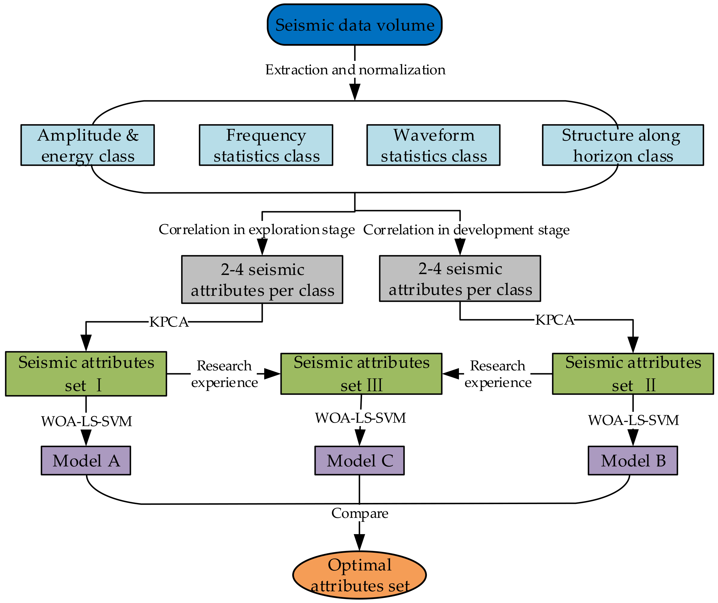
  • Based on the amplitude and energy class, frequency statistics class, waveform statistics class, and structure along horizon class, multiple more commonly used seismic attributes were extracted from the seismic data volume and normalized to the 0–1 interval (i.e., the data were mapped to the [0, 1] interval uniformly). The purpose of normalization was to limit the preprocessed data to a certain range, thus eliminating the adverse effects caused by odd sample data to facilitate later data analysis.
  • Coal thickness correlation analysis was separately performed for each major class of seismic attributes, and two to four seismic attributes with high correlation and relative independence of changes in the coal thickness data exposed in the coal exploration stage, were preferably selected to facilitate precise prediction of the coal seam thickness characteristics and improve the accuracy of their description.
  • Because of the nonlinear relationship between coal thickness and multiple seismic attributes, a set of seismic attribute sets was developed using attribute dimension reduction algorithms, such as KPCA, to select the primary seismic attributes whose cumulative principal element variance contribution values exceeded a set threshold (95%) as a set of input parameters for the coal thickness prediction model.
  • Moreover, the seismic attributes were preferentially selected by amplitude and energy and other major classes (i.e., the cumulative coal thickness data obtained in the exploration and development stages were used as samples), and two to four seismic attributes with high correlation and relative independence of the coal thickness variation were selected from each major category of seismic attributes. The novel seismic attribute combinations were reacquired using the dimension reduction algorithm for seismic attributes. Furthermore, based on the results of the two attribute preferences, a third set of seismic attribute combinations was obtained by combining seismic attribute selection experience and regional seismic attribute characteristics in similar previous studies.
  • The coal thickness data and corresponding seismic attribute data obtained in the exploration and development stages of the study area were used as training samples, and a training model based on the prediction of coal thickness between coal thickness and multiple seismic attributes was established according to three different combinations of seismic attributes. The thickness of the coal seams at the geological sampling points in the first mining face in the mining stage was predicted.
  • Comparing the thickness predicted by the three prediction models with the actual coal thickness data obtained for the first mining face, the seismic attribute combination with the highest prediction accuracy was selected as the base parameter for the prediction model of coal thickness in the working faces in the later mining stages.

Appendix B. Whale Optimization Algorithm Pseudocode

  • Input: Fitness function, whale population
  • Output: Optimal solution
  • Step 1. Set the parameter values involved in the algorithm: the population size N, the maximum number of iterations Max_iter, the variation scale factor F, the constant coefficient b of the spiral formula, and the positions of all whale individuals within the population, and randomly generate the relevant parameter values of A, C, a, p and l.
  • Step 2. Randomly generate the positions of all individuals in the population and calculate their fitness, then record the best whale positions and their fitness values.
  • Step 3. while (t < Max_iter)
  • Step 4. for j = 1:N
  • Step 5. if p < 0.5
  • Step 6. if abs(A) ≥ 1
  • Step 7. Update the current whale position based on a random whale position
  • Step 8. else abs(A) < 1
  • Step 9. Update the current whale position based on the prey location
  • Step 10. end
  • Step 11. end
  • Step 12. else p ≥ 0.5
  • Step 13. Update the whale position according to Archimedes’ spiral formula
  • Step 14. t = t + 1
  • Step 15. end
  • Step 16. Return the optimal solution

Appendix C. Construction Process of the WOA–LS-SVM Coal Thickness Prediction Model

  • Preprocess the coal thickness data and seismic attribute data to obtain the input sample dataset.
  • Initialize the whale population with the empirical values of γ and δ: set the population size N, spiral formula coefficient b, number of iterations t and Max_iter, variation scale factor F, spiral formula constant coefficient, and positions of all whale individuals in the population. Randomly produce the relevant parameter values of A, C, a, p, and l.
  • Train the LS-SVM prediction models using the processed datasets.
  • Calculate the fitness value of all individual whales in the population according to the fitness function (Equation (C1)), and record the current best fitness value and the best whale location:
f = 1 N i N y i y ^ i y i
where N is the number of training samples, yi is the actual value and y ^ i is the predicted value.
  • Update the values of parameters A, C, and a according to Equations (3) and (4), respectively, and generate the values of p and l.
  • If p < 0.5 and |A| < 1, update the whale individual position according to the following equation:
X t + 1 = X * t A D + λ
If p < 0.5 and |A| > 1, randomly select the whale individual position from the current population space and update the whale position according to the following equation: K x m , x n = φ x m T φ x n , m , n = 1 , N .
  • If p ≥ 0.5, update the whale position according to the following equation:
    X t + 1 = D b l cos 2 π l + X * t
  • Determine whether the maximum number of iterations has been reached. If so, the algorithm optimization is complete; otherwise, return to step (3) and continue the execution.
  • The optimal whale individual positions are saved as two parameters of the LS-SVM, and then the WOA–LS-SVM prediction model is constructed.

Appendix D. Classes and Preliminary Data of Seismic Attributes

Table A1. Extracted seismic attributes of T5 waves along horizon.
Classes of
Seismic Attributes
Seismic Attributes
Amplitude and
energy class
Amplitudes, average energy, average magnitude, average peak value, average positive amplitude, average positive peak value, maximum amplitude, mean amplitude, median, minimum amplitude, rms amplitude, standard deviation of amplitude, sum of amplitudes, sum of magnitudes, sum of positive, ari poststack amplitude, geo poststack amplitude, ins poststack amplitude, std poststack amplitude, ins poststack amplitude, half energy, extract value, geometric mean, harmonic mean
Frequency classArc length, dominant frequency-rms amplitude, envelope-rms amplitude, instantaneous bandwidth rms amplitude, instantaneous frequency rms amplitude
Waveform
statistics class
Interval average arithmetic, loop asymmetry, loop kurtosis, lower loop area, lower loop duration, upper loop area, upper loop duration, upper loop skewness
Structure along
horizon class
Ins curvature, contour curvature, curvedness, dip, dip azimuth, edge preserving, filter mean irregular, edge preserving filter mean regular, edge preserving filter median irregular, edge preserving filter median regular, Gaussian curvature, Lambertian reflectance, local variability, max filter, maximum curvature, mean curvature, mean filter, median filter, min filter minimum curvature, most negative curvature, most positive curvature, Prewitt filter (crossline), Prewitt filter (inline), Roberts filter (A), Roberts filter (B), second-order derivative, shape index, Sobel filter (crossline), Sobel filter (inline), strike, strike curvature, throw
Table A2. Preliminary seismic attribute data corresponding to geological boreholes in the exploration stage (after normalization).
BoreholeAverage EnergyAverage Positive Peak ValueMaximum AmplitudeRms
Amplitude
Envelope Rms AmplitudeArc LengthUpper Loop AreaInterval AverageMedian FilterMean FilterMean Regular
10-10.247340.370670.360990.366700.423140.591330.241580.317600.227880.228950.22243
10-20.257520.362650.379800.378410.448910.479260.322740.333180.362450.363970.37221
10-30.206100.282330.270680.317460.331840.425340.281820.356320.553900.553910.55196
10-40.745980.896220.902110.821380.898721.000000.709940.760170.637920.645080.63157
10-50.428860.555460.566410.555750.588810.647470.458560.545450.702600.702720.70139
11-10.168290.169140.175790.269460.244800.160390.223230.355340.124540.123360.12462
11-30.225550.255400.263700.341060.331550.273190.281820.393190.033460.032300.02867
12-10.000000.298770.035510.000000.000000.084010.013130.000000.080300.085950.00957
12-20.195450.259260.277720.304240.310360.327160.199330.327980.126390.129170.10967
12-30.515460.577050.568360.634630.621760.449450.622500.691120.553900.553910.55196
12-40.467440.571500.588220.591620.618420.568830.552630.624080.874350.877310.86077
E20.138150.162310.157500.228850.226010.258560.149550.260730.752790.758830.74632
10 + 10.894190.952070.990290.928371.000000.986160.883210.843820.855020.857560.85221
Table A3. Preliminary seismic attribute data corresponding to geological boreholes in the development stage (after normalization).
Borehole/Coal SpotStd
Poststack
Amplitude
Ins
Poststack
Amplitude
Maximum
Amplitude
Geo
Poststack
Amplitude
Average
Energy
Envelope
Rms
Amplitude
Arc
Length
Upper
Loop
Area
Interval
Average
Arithmetic
Shape
Index
Strike
10-10.548420.343900.360990.712130.247340.423130.591330.241580.317600.594960.81939
10-20.536050.219980.379800.694210.257520.448910.479260.322740.333180.097680.83471
10-30.378790.409400.270680.484310.206100.331840.425340.281820.356320.413220.51014
10-40.917800.950750.902110.784630.745980.898721.000000.709940.760170.118200.99252
10-50.621190.568420.566410.749250.428860.588810.647470.458560.545450.836560.00000
11-10.269550.309580.175790.511970.168290.244800.160390.223230.355340.797310.88172
11-30.395950.385640.263700.629880.225550.331550.273190.281820.393190.873530.00000
12-10.000000.053970.035510.252420.000000.000000.084010.013130.000000.438950.05751
12-20.304520.365910.277720.518040.195450.310360.327160.199330.327980.790780.00000
12-30.639740.669290.568360.571370.515460.621760.449450.622500.691120.413220.51014
12-40.617100.614620.588220.726380.467440.618420.568830.552620.624080.438580.59334
E21.000000.135530.157500.512510.138150.226010.258560.149550.260730.000000.11328
10 + 10.398761.000000.990291.000000.894191.000000.986160.883210.843820.440320.63369
W1-10.398760.358310.392450.625860.322610.446800.403070.385800.459600.869720.17550
W1-20.278050.246000.212910.523010.146220.288600.356970.120850.259760.285880.89670
W1-30.576200.450180.550410.709070.398770.570750.673390.420440.497100.440330.45652
W1-40.485230.522230.418890.703370.371350.480710.347710.467310.579330.801770.81130
W2-10.315990.322680.245200.593850.220420.334810.207090.303180.441530.674150.00000
W2-20.384920.402850.274910.595700.196770.328010.387840.203550.327540.873530.00000
W2-30.369870.397780.269160.556240.239260.331490.289300.359690.443661.000000.00000
W2-40.558760.530610.419790.660160.319210.484050.541150.333660.450000.880650.00000
W2-50.595360.625010.526840.705420.402910.559710.618820.441610.531190.190910.00000
W3-10.138050.185050.027930.416600.100700.078470.000000.196350.309190.078200.61462
W3-20.361250.499170.384140.572240.322190.115540.357020.437770.507240.802950.51014
W3-30.447830.489560.373240.602310.331420.433130.315450.436240.534020.439860.25497
W3-40.299660.289580.146460.599060.209220.251240.032030.378020.461030.439900.76522
W3-50.441920.467990.348780.000000.261370.397800.443620.292710.399160.190910.00000
W3-60.548810.585100.509700.636870.392130.567660.625860.404410.509230.800460.00000
W3-70.435910.462140.342150.667110.225860.380990.499720.221750.339610.439690.15054
J10.495060.555670.448210.676080.383040.838500.417700.501760.573900.800530.70112
J20.828220.866130.870870.953290.832470.877220.669270.910780.963770.249160.32135
J30.913870.782991.000000.922601.000000.996900.811931.000001.000000.126600.42329
J40.815260.966730.914340.831960.811600.893180.846420.807720.844670.102790.51014
Table A4. Selection of seismic attributes in the representative study of seismic multi-attribute coal thickness prediction.
No.Principal ResearchersExtracted Seismic AttributesAdopted Seismic AttributesYearStudy Area
1Cui, WangAmplitude, dominant frequency, dominant frequency amplitude, average frequency, low-frequency
(5–35 Hz) bandwidth energy
Amplitude, dominant frequency, dominant frequency amplitude, average frequency, low-frequency
(5–35 Hz) bandwidth energy
1997Zhangxiaolou mine in Xuzhou, No. 2 coal seam
2Han, Zhang, LiEight types of time domains, nine types of frequency domains, three types of fractal parametersPeak and trough amplitude, average frequency, energy of dominant-frequency bandwidth, energy of low-frequency bandwidth, peak frequency2001Coalfield, No. 2 coal seam
3Meng, Guo, Wang et al.15 types of amplitude class, five types of complex trace statistics, eight types of spectral statisticsAverage instantaneous frequency, average peak amplitude, kurtosis of amplitude, maximum absolute amplitude, maximum peak amplitude, maximum trough amplitude, instantaneous frequency slope, amplitude variation2006Xieqiao mine in Huainan, 13-1 coal seam
4Hu, Qian, ZhongPeak and trough amplitude, average frequency, energy of dominant-frequency bandwidth, energy of low-frequency bandwidth, peak frequencyPeak and trough amplitude, average frequency, energy of dominant-frequency bandwidth, energy of low-frequency bandwidth, peak frequency2010Huainan coalfield
5Wang, Cui, Chen18 types of seismic wave kinematics, dynamics, time domain and frequency domainAverage frequency phase, main frequency phase, dominant frequency, correlation coefficient, two-dimensional fractal parameters, broadband total energy, capacity dimension2010East 6 mining section, Liangjia coal mine in Longkou
6Suo, Chang, Peng et al.Maximum absolute amplitude, apparent time difference of reflection at the top–bottom interface of coal seamMaximum absolute amplitude, apparent time difference of reflection at the top–bottom interface of coal seam2011A coalmine in Yangquan, No. 15 coal seam
7Du63 types of instantaneous, wavelet, amplitude statistics and spectral attributesUpper and lower limit frequencies, apparent polarity, dominant power spectrum, response frequency, root mean square amplitude, smoothing frequency, sum of autocorrelation, relative layer thickness2013Taoyuan coalmine in Huaibei
8Chen, Yang, Zhang et al.Maximum amplitude, maximum number, positive polarity amplitude, instantaneous phase, instantaneous frequency, average number, average wave crest number, root mean square amplitude, arc length, minimum amplitudeMaximum number, instantaneous frequency, average peak number, arc length2015First mining section, Shilawusu coal mine, 4-1 coal seam
9Xu, Han, Zhang et al.17 types of amplitude classes, two types of complex trace statistics, one type of spectral statisticsAverage energy, average negative phase amplitude, average trough amplitude, average zero crossing trough, instantaneous amplitude, relative acoustic impedance, standard deviation of amplitude, minimum amplitude2017West second mining section, coal mine in Huainan, A group coal seam
10ShanAmplitude, frequency, phase, spectrum statistics, etc.Derivative instantaneous, amplitude phase, amplitude weighted cosine, dominant frequency, cosine instantaneous phase, quadrature trace, filter 5/10–15/20, filter 45/50–55/602021Coal mine in Xinjiang,
A3 coal seam

References

  1. Yuan, L. Scientific conception of precision coal mining. J. China Coal Soc. 2017, 42, 1–7. [Google Scholar] [CrossRef]
  2. Yuan, L.; Jiang, Y.D.; Wang, K.; Zhao, Y.X.; Hao, X.J.; Xu, C. Precision exploitation and utilization of closed/abandoned mine resources in China. J. China Coal Soc. 2018, 43, 14–20. [Google Scholar] [CrossRef]
  3. Shang, X.Q.; Yang, H.Y.; Ai, G.; Zhang, Y.G.; Zhu, G.A. Study on the evolution and impact of mining-induced stress in coal thickness variation area. China Min. Mag. 2020, 29, 148–151, 157. [Google Scholar] [CrossRef]
  4. Cui, W.X.; Wang, B.L.; Wang, Y.H. High-precision inversion method of coal seam thickness based on transmission channel wave. J. China Coal Soc. 2020, 45, 2482–2490. [Google Scholar] [CrossRef]
  5. Huang, Y.; Yan, L.; Cheng, Y.; Qi, X.; Li, Z. Coal Thickness Prediction Method Based on VMD and LSTM. Electronics 2022, 11, 232. [Google Scholar] [CrossRef]
  6. Ricker, N. The Form and Laws of Propagation of Seismic Wavelets. Geophysics 1953, 18, 10–40. [Google Scholar] [CrossRef]
  7. Widess, M.B. How thin is a thin bed. Geophysics 1973, 38, 1176–1180. [Google Scholar] [CrossRef]
  8. Ruter, H.; Schepers, R. Investigation of the seismic response of cyclically layered carboniferous rock by means of synthetic seismograms. Int. J. Rock Mech. Min. Sci. Geomech. Abstr. 1978, 15, 92. [Google Scholar] [CrossRef]
  9. Koefoed, O.; De Voogd, N. The linear properties of thin layers, with an application to synthetic seismograms over coal seams. Geophysics 1980, 45, 1254–1268. [Google Scholar] [CrossRef]
  10. Cheng, Z.Q.; Wu, Y.F.; Zhao, Z.Q.; Zhang, S.S.; Wang, Z.R.; Ning, L. Quantitative interpretating method of coal using seismic reflected wave. Acta Geophys. Sin. 1991, 34, 657–662. [Google Scholar]
  11. Dong, S.H. Seismic Data on Coal Seam Lateral Prediction and Evaluation Methods; China University of Mining and Technology Press: Xuzhou, China, 2004; pp. 23–95. [Google Scholar]
  12. Suo, C.H.; Chang, S.L.; Peng, S.M.; Duan, R.T.; Wang, G.M. Study and Application of Seismic Attributes on Coal Seam Thickness Prediction. Sci. Technol. Eng. 2011, 11, 8429–8433. [Google Scholar] [CrossRef]
  13. Meng, F.B. Numerical Simulation and Seismic Response Analysis of coal seam thickness variation. Chin. J. Eng. Geophys. 2018, 15, 677–685. [Google Scholar] [CrossRef]
  14. Liu, T.F.; Chen, B.; Fu, J.S. Spectral moment method for seismic inversion of coal seam thickness and its application. In A Collection of Technical Papers on Geophysical Lithology Exploration in Coalfield; Coal Industry Press: Beijing, China, 1996; pp. 135–146. [Google Scholar]
  15. Liu, J.H.; Liu, T.F. Study of the trace integration method for predicting coal seam thickness. J. China Univ. Min. Technol. 1996, 25, 73–76. [Google Scholar]
  16. Peng, S.P.; Zou, G.G.; Li, Q.L. Seam Thickness Prediction Methods Based on the Logging Constrained Seismic Inversion. J. China Univ. Min. Technol. 2008, 37, 729–733. [Google Scholar] [CrossRef]
  17. Cui, R.F.; Zhong, Q.T.; Li, J.P. Coal thickness interpretation prediction using seismic data. Coal Geol. Explor. 2002, 30, 54–57. [Google Scholar]
  18. Meng, Z.P.; Guo, Y.S.; Wang, Y.; Pan, J.N.; Lu, J. Prediction models of coal thickness based on seismic attributions and their applications. Chin. J. Geophys. 2006, 49, 512–517. [Google Scholar] [CrossRef]
  19. Wang, X.; Chen, T. Quantitative Prediction of Tectonic Coal Thickness Based on FNN and Seismic Attributes. J. Inf. Comput. Sci. 2014, 11, 3653–3662. [Google Scholar] [CrossRef]
  20. Wang, X.; Chen, T.J.; Xu, H. Thickness distribution prediction for tectonically deformed coal with a deep belief network: A case study. Energies 2020, 13, 1169. [Google Scholar] [CrossRef] [Green Version]
  21. Shan, R. Application of Multi-group Seam Thickness Prediction in CJT Coal Mine. IOP Conf. Ser. Earth Environ. Sci. 2020, 525, 012091. [Google Scholar] [CrossRef]
  22. Wang, X.; Li, Y.; Chen, T.J.; Yan, Q.Y.; Li, M. Quantitative thickness prediction of tectonically deformed coal using Extreme Learning Machine and Principal Component Analysis: A case study. Comput. Geosci. 2017, 101, 38–47. [Google Scholar] [CrossRef]
  23. Li, Z.W.; Xia, S.X.; Niu, Q.; Xia, Z.G. Coal Thickness Prediction Based on Support Vector Machine Regression. In Proceedings of the Eighth Acis International Conference on Software Engineering, Qingdao, China, 30 July 2007; IEEE: Qingdao, China, 2007. [Google Scholar] [CrossRef]
  24. Qi, A.L.; Kang, W.H.; Zhang, G.M.; Lei, H.J. Coal seam thickness prediction based on transition probability of structural elements. Appl. Sci. 2019, 9, 1144. [Google Scholar] [CrossRef] [Green Version]
  25. Zeng, A.P.; Zhang, J.W.; Ren, E.M.; Liu, T.; Jiang, F.; Liu, X.J.; Jiang, F. Research on coal thickness prediction method based on VMD and SVM. Coal Geol. Explor. 2021, 49, 243–250. [Google Scholar] [CrossRef]
  26. Zheng, H.Z.; Wei, C.J.; Wang, S.H. Seismic attribute optimization research based on principal component analysis and kernel principal component analysis. J. Qingdao Univ. 2017, 30, 76–80. [Google Scholar] [CrossRef]
  27. Li, H.X.; Wu, S.Y. Attribute reduction and optimization for massive seismic data based on principal component analysis. China Earthq. Eng. J. 2019, 41, 757–762. [Google Scholar] [CrossRef]
  28. Chen, Y.K.; Yang, Y.G.; Zhang, X.; Zhang, H. Forecasting of coal thickness based on rough set and LS-SVM. Prog. Geophys. 2015, 30, 2136–2141. [Google Scholar] [CrossRef]
  29. Fan, J.; Wang, X.; Xu, H. Prediction method of tectonic coal thickness based on particle swarm optimized hybrid kernel extreme learning machine. J. Comput. Appl. 2018, 38, 1820. [Google Scholar] [CrossRef]
  30. Zhou, X.J.; Gao, F.; Fang, X.; Lan, Z.H. Improved bat algorithm for UAV path planning in three-dimensional space. IEEE Access 2021, 9, 20100–20116. [Google Scholar] [CrossRef]
  31. Karaboga, D.; Basturk, B. A powerful and efficient algorithm for numerical function optimization: Artificial bee colony (ABC) algorithm. J. Glob. Optim. 2007, 39, 459–471. [Google Scholar] [CrossRef]
  32. Mirjalili, S. How effective is the Grey Wolf optimizer in training multi-layer perceptron. Appl. Intell. 2015, 43, 150–161. [Google Scholar] [CrossRef]
  33. Houssein, E.H.; Ahmed, M.M.; Elaziz, M.A.; Ewees, A.A.; Ghoniem, R.M. Solving Multi-Objective Problems Using Bird Swarm Algorithm. IEEE Access 2021, 9, 36382–36398. [Google Scholar] [CrossRef]
  34. Mirjalili, S.; Lewis, A. The Whale Optimization Algorithm. Adv. Eng. Softw. 2016, 95, 51–67. [Google Scholar] [CrossRef]
  35. Kaur, G.; Arora, S. Chaotic Whale Optimization Algorithm. J. Comput. Des. Eng. 2018, 5, 275–284. [Google Scholar] [CrossRef]
  36. Mafarja, M.M.; Mirjalili, S. Hybrid Whale Optimization Algorithm with simulated annealing for feature selection. Neurocomputing 2017, 260, 302–312. [Google Scholar] [CrossRef]
  37. Suykens, J.A.K.; Vangestel, T.; Debrabanter, J. Least Squares Support Vector Machines; World Scientific: Singapore, 2002; pp. 1–26. [Google Scholar]
Figure 1. Flow chart of the comprehensive optimization framework for seismic attribute combination.
Energies 15 07324 g001
Figure 2. Flow chart of the whale-optimization-algorithm-optimized least squares support vector machine (WOA–LS-SVM) coal thickness prediction model construction.
Energies 15 07324 g002
Figure 3. Location of mining engineering in the study area.
Energies 15 07324 g003
Figure 4. Cumulative variance contribution of the seismic attributes of kernel principal component analysis in the exploration stage.
Energies 15 07324 g004
Figure 5. Cumulative variance contribution of the seismic attributes of kernel principal component analysis in the development stage.
Energies 15 07324 g005
Figure 6. (a) Actual coal thickness distribution, (b) predicted coal thickness distribution—Model A, (c) predicted coal thickness distribution—Model B, and (d) predicted coal thickness distribution—Model C.
Energies 15 07324 g006aEnergies 15 07324 g006b
Figure 7. (a) Actual coal thickness distribution and (b) predicted coal thickness distribution.
Energies 15 07324 g007
Table 1. Seismic attribute correlation analysis in the exploration stage.
Classes of Seismic AttributesSeismic AttributesCorrelation Coefficient with Coal Thickness
Amplitude and
energy class
Average energy−0.69775
Average positive peak value−0.66054
Maximum amplitude−0.64955
Rms amplitude−0.63253
Frequency classEnvelope-rms amplitude−0.63126
Arc length−0.57008
Waveform
statistics class
Upper loop area−0.65711
Interval average–arithmetic−0.57268
Structure along
horizon class
Median filter−0.28807
Mean filter−0.28726
Mean regular−0.28664
Table 2. Seismic attribute correlation analysis in the development stage.
Class of Seismic AttributesSeismic AttributesCorrelation Coefficient with Coal Thickness
Amplitude and energy classStd poststack amplitude−0.46954
Ins poststack amplitude−0.45588
Maximum amplitude−0.44909
Geo poststack amplitude−0.44728
Average energy−0.44292
Frequency classEnvelope-rms amplitude−0.45009
Arc length−0.44547
Waveform statistics classUpper loop area−0.38463
Interval average–arithmetic−0.34505
Structure along horizon classShape index−0.12820
Strike0.11526
Table 3. Training results of the whale optimization algorithm for three input sample datasets.
Coal Thickness
Prediction Models
Seismic Attribute SetPenalty Factor γKernel Function Parameter σ2
Model ASet I26.3548.24
Model BSet II67.19257.05
Model CSet III76.67330.56
Table 4. Comparison of coal thickness prediction results of typical sampling points in the secondary mining face.
No.Actual Thickness (m)Predicted Thickness (m)Absolute Error (m)Relative Error
(%)
cc1023.43.10.38.82
cc1073.63.80.25.56
cc1083.83.800.00
cc1164.04.10.12.50
cc1223.73.80.12.70
cc1274.34.00.36.98
cc1314.23.90.37.14
cc2013.43.30.12.94
cc2043.73.90.25.41
cc2072.63.10.519.23
cc2123.63.50.12.78
cc3033.73.60.12.70
cc3083.53.500.00
cc3143.73.90.25.41
cc3193.94.20.37.69
cc3243.93.80.12.56
cc3283.73.700.00
cc4013.43.400.00
cc40633.20.26.67
cc4122.32.80.521.74
cc4132.33.00.730.43
cc4173.83.70.12.63
cc4213.94.00.12.56
cc4253.23.60.412.50
cc4303.93.900.00
cc4353.73.60.12.70
cc5013.53.500.00
cc5073.83.90.12.63
cc5103.03.20.26.67
cc5153.53.60.12.86
cc5214.03.80.25.00
cc5254.04.000.00
cc5284.24.30.12.38
cc5313.740.38.11
cc5344.23.90.37.14
cc5363.83.70.12.63
Publisher’s Note: MDPI stays neutral with regard to jurisdictional claims in published maps and institutional affiliations.

